Adaptive Beamforming Algorithms for Cancellation
of Multiple Interference Signals
Lay Teen Ong*
Abstract—This paper proposes a fast Minimum-Variance-Distortionless-Response (MVDR) beam-forming algorithm for an antenna array for cancellation of multiple interference signals. The proposed algorithm uses Sample-Average Estimate (SAE) of the data covariance matrix and reduces its compu-tational effort by applying the Matrix-Inversion-Lemma (MIL) to its covariance Matrix Inversion (MI) operation. The proposed algorithm is compared to two SAE-based algorithms: the Sample Matrix Inversion (SMI) algorithm that requires an MI operation and the Auxiliary Vector (AV) algorithm that does not need an MI operation. A non-SAE based algorithm using the Least Mean Square (LMS) method is also included for comparison. Simulation results show that the proposed algorithm converges slower than the SMI scheme but outperforms the AV and LMS schemes during the transient phase. Once convergence is achieved, the proposed algorithm converges to a better Mean Square Error than the rest of the algorithms evaluated.
1. INTRODUCTION
Adaptive beamforming applied to antenna arrays has been a popular approach to enhance the desired signal in the presence of interference signals. The technique applied to Radar or Wireless Communications Systems enhances performance [1–5]. Minimum-Variance-Distortionless-Response (MVDR) is a classical method used in adaptive beamforming of an antenna array [6–9]. The array weights of the MVDR beamformer can be adapted through various algorithms. For example, the Sample Matrix Inversion (SMI) based algorithm is a fast adaptive beamforming/nulling technique because it directly calculates the covariance matrix [10–12]. SMI avoids the problem of eigenvalue spread that often limits the convergence rate for close-loop algorithms such as the Least Mean Square (LMS) approach. In practice, the SMI approach makes use of the Sample-Average Estimate (SAE) of the data covariance matrix and the numerical inversion of the covariance matrix to find optimum weight values. The Auxiliary Vector (AV) algorithm is another fast beamforming method that uses the SAE of the covariance matrix to approach the MVDR optimum solution and does not need a numerical inversion operation [13, 14]. The results in [13] have shown that the sequence of AV filter estimators provide favorable bias/variance and have better mean-square estimation error than LMS, Recursive Least Squares (RLS), SMI and orthogonal multistage decomposition filter estimators. One notes that the LMS algorithm has been widely used because of its simplicity in implementation [7]. However, the trade-offs of the LMS method includes its convergence speed and its dependency on the eigvenvalue spread of the input signals. The RLS method uses a recursive matrix inversion algorithm that is more complicated but efficient than LMS [7, 13]. The above-mentioned algorithms form a class of algorithms that can be implemented effectively using Digital beamforming (DBF) technology. DBF has gained popularity for enabling the flexibility and configurability of a receiving array system [15–18]. For DBF, the array system needs a receiver at each element to receive and process the arriving signals. The
Received 12 June 2015, Accepted 9 August 2015, Scheduled 18 August 2015 * Corresponding author: Lay Teen Ong ([email protected]).
receiver down converts the received signal from the array element to an intermediate frequency (IF) band and then further converts the analogue signal to digital signals. The digitized signals from all the receivers are then processed by the beamforming algorithm in a fast digital processor. In contrast, in the traditional phased-array beamforming (PAB) technology, the signals received by the array are shifted in phase and/or amplitude by a digital or analogue device at each element, then summed and down converted to an IF band before conversion to digital signals by a single receiver. The traditional PAB technology has retained its popularity because it can be less expensive in terms of hardware but this is at the expense of its design flexibility. Several evolutionary algorithms such as the Genetic algorithms (GA) and the Particle-Swarm Optimization (PSO) have shown to be effective in implementation for the PAB technology [19, 21]. In general, the GA/PSO approach is constrained to making small (or fixed) amplitude and small phase perturbations at each element [19–21].
This paper proposes a fast and computationally efficient beamforming algorithm that uses the SAE approach and applies the Matrix-Inversion-Lemma (MIL) in the MVDR solution for DBF. Some earlier works, such as [3] and [22] had verified the computationally efficient of the MIL implementation for adaptive beamformers but our work has differences compared to these works. The classical work in [3] had shown that a MIL adaptive algorithm, compared to other classical algorithms such as the Applebaum adaptive control loop method [1], achieves a rapid convergence by using the system gain of a radar array system. The work in [22] implemented MIL in the linearly constrained minimum variance (LCMV) beamformer. The LCMV method is a generalized form of the MVDR beamformer, allowing for additional constraints to act on known interference and/or additional desired signals [7]. [22] studied the complexity gain of using MIL for various array sizes and various numbers of constraints but did not make comparison to other adaptive algorithms. In our paper, we compare the MIL approach to the more recent and favorable AV algorithm for a MVDR beamformer. We also include the conventional SMI algorithm and a low complexity LMS algorithm for comparison. Our MVDR beamformer is considered for the pre-correlation stage of an antenna array spread spectrum (SS) system and is vulnerable to strong interference signals due to its weak received desired signal. The main benefit of using antenna array based adaptive beamforming in SS system is the extra degree of freedom in spatial and temporal domain for mitigation of interference while maintaining a main antenna beam to the desired signal [23, 24]. However, this approach increases hardware and computational processing complexity. Therefore, improvements to receiver hardware, antenna selection strategies and adaptive beamforming algorithms are imperative [5, 18]. Herein, our paper focuses on the computation processing efficiency of the MVDR beamforming algorithms in terms of their convergence rate analysis and their interference cancellation performance in environments of multiple interference signals. In addition, we analyses their adaption rate in terms of the array’s weights-convergence (instead of the system gain parameter). Finally, we show that the Mean Square Error (MSE) of the array weights is a better figure-of-merit (FOM) than the array gain pattern for assessing beamformers, especially in scenarios where there are multiple interference signals.
2. SIGNAL MODEL & PROBLEM FORMATION 2.1. Signal Model
We consider a Uniform Circular Array (UCA) with N antenna elements positioned equidistant from each other and at radiusr from the centre of the array. The array receives one desired signal andM−1 interference signals. The received array signal vector x(t) at time tcan be written as [17, 25]
x(t) =A(θ, φ) s(t) +n(t), (1) where A(θ, φ) = [a(θ0, φ0), a(θ1, φ1), . . . ,a(θM−1, φM−1)] is an N × M matrix whose columns,
with zero mean and variance σn2. The output of the beamformer is y(t) = w(t)Hx(t) where
w(t) = [w1(t), w2(t) ,· · · , wN(t)] is a×N weight vector whose components correspond to the weights of the beamformer andHdenotes Hermitian transpose. The exact covariance matrix of the total received signal is R=Ex(t)xH(t) whereE(.) denotes the expectation operator.
2.2. MVDR Problem Formation
The MVDR method minimizes the output power of the array subject to a constraint of unity gain in the look direction of the array [1, 7]. The problem formulation is,
min
w w
HRw s.t. wHa(θ
0, φ0) = 1, (2)
where a(θ0, φ0) is the steering vector of the desired signal. The solution to the optimization problem can be shown to be
w= R
−1a(θ 0, φ0)
a(θ0, φ0)HR−1a(θ0, φ0)
. (3)
Subsequently, for adaptive beamforming, iterative weight values w(t) that based on the MVDR solution (3) can be computed. t denotes the sample instance. The next section discusses the adaptive beamforming algorithms considered in this work.
3. THE ALGORITHMS
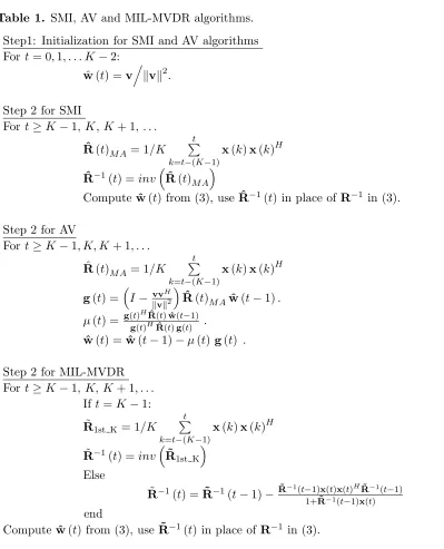
This section describes our proposed MIL-MVDR algorithm and two SAE based algorithms, namely the SMI and the AV algorithm. For comparison to a non-SAE based algorithm, the LMS algorithm is also included. The MIL-MVDR, SMI and AV algorithms are outlined in Table 1. Note that the initial estimate weight, wˆ(0) =v/v2, where v=a(θ0, φ0), is applied to all the algorithms studied here.
3.1. The Sample Matrix Inversion Algorithm
A SMI method uses an SAE approach to estimate its data covariance matrix [10],
ˆ
R= 1/K K
k=1
x(k)x(k)H, (4)
where K is the number of snapshots observed over a data record size. Rˆ is then substituted into the MVDR solution (3) to obtain an estimate weight, wˆ. The SMI method requires K > 2N samples of data to achieve an average loss of less than 3 dB [10] and a matrix inversion operation, inv(), for wˆ
computation. To enable meaningful comparison to the MIL-MVDR, AV and LMS algorithms, we adopt a moving average (MA) approach to computeRˆ iteratively. That is,Rˆ is computed over a moving, but fixed K-sample of data block, and is denoted as Rˆ(t)MA. The SMI based algorithm, denoted as SMI, is outlined in Table 1.
3.2. The Auxiliary-Vector Filtering Algorithm
3.3. The Proposed MIL-MVDR Algorithm
Our proposed algorithm computes data covariance matrix, R˜1st K, and its inversion only for the first available K samples of data. After K sample instances, we uses the matrix-inversion-lemma (MIL) function to iteratively compute the inverse value of the data covariance matrix (5). Therefore, the MIL approach reduces its computational complexity compared to the SMI using a matrix inversion. In addition, the computational load of the MIL-MVDR algorithm is lower than the SMI algorithm as the SMI method computes Rˆ (t)MA and its inverse at every sample instance. Our proposed algorithm, denoted as MIL-MVDR, is summarized in Table 1.
Table 1. SMI, AV and MIL-MVDR algorithms. Step1: Initialization for SMI and AV algorithms Fort= 0,1, . . . K −2:
ˆ
w(t) =v
v2.
Step 2 for SMI
Fort≥K−1,K,K+ 1, . . .
ˆ
R(t)MA = 1/K t k=t−(K−1)
x(k)x(k)H
ˆ
R−1(t) =inv Rˆ (t)MA
Computewˆ (t) from (3), useRˆ−1(t) in place of R−1 in (3).
Step 2 for AV
Fort≥K−1, K, K+ 1, . . . ˆ
R(t)MA = 1/K t k=t−(K−1)
x(k)x(k)H
g(t) = I−vvH
v2
ˆ
R(t)MAwˆ (t−1).
μ(t) = g(gt)HRˆ(t)wˆ(t−1) (t)HRˆ(t)g(t) .
ˆ
w(t) =wˆ (t−1)−μ(t) g(t) .
Step 2 for MIL-MVDR Fort≥K−1, K, K+ 1, . . .
Ift=K−1: ˜
R1st K = 1/K t k=t−(K−1)
x(k)x(k)H
˜
R−1(t) =inv R˜1st K
Else
˜
R−1(t) =R˜−1(t−1)−R˜−1(t−1)x(t)x(t)HR˜−1(t−1)
1+R˜−1(t−1)x(t) (5) end
Computewˆ (t) from (3), useR˜−1(t) in place of R−1 in (3).
3.4. The LMS Algorithm
Step1: Initialization, t= 0
ˆ
w(t) =v
v2.
Step 2 for LMS, fort≥1,2, . . .
ˆ w(t) =
I−vv
H
v2 wˆ(t−1)−μx(t)x(t)
Hwˆ (t−1)+ v v2
and 1/2λmax≥ μ ≥ 0, whereλmax is the largest eigenvalue of the data correlation matrix.
In contrast to the SMI and AV algorithm, the covariance matrix of the signal is computed at every sample instance instead of over a block of K samples.
4. SIMULATIONS AND RESULTS ANALYSIS
We evaluate the performance of the beamformer implemented using the MIL-MVDR, SMI, AV and LMS algorithms in an environment with multiple interference signals. For reference, an ideal MVDR algorithm is included. The algorithms are simulated using Matlab software running on an Intel i7 CPU-3.4 GHz General Purpose Computer. We use the MSE and the Array Pattern as two different Figure-of-Merits to measure the performance of the beamformer. We also evaluate the computational complexity of the algorithm based on the CPU time.
A UCA antenna with 8 elements and r = 0.5λ is used. We consider an 8-element array for its practical realization in terms of compactness and interference mitigation performance when used in SS systems for GNSS applications [26–28]. The desired signal arrives from the broadside direction (0◦, 0◦) of the array and its signal power is 20 dB below the noise level. We consider a total of four interference signals and each signal has an interference-to-noise ratio of 40 dB. We evaluate four different scenarios where there is 1, 2, 3 or 4 interference signals corresponding to scenario Zone 1, 2, 3 and 4 respectively. Table 2 defines the angle setting of the scenarios. The data record size,K, is set to 256. The simulation is repeated 1000 trials for average weight analysis.
Table 2. Interference bearing setting for Zone 1 to 4.
Zone # (Elevation, Azimuth): (θ, φ) 1 (80◦, 0◦)
2 (80◦, 0◦), (70◦, 0◦)
3 (80◦, 0◦), (70◦, 0◦), (−60◦,0◦)
4 (80◦, 0◦), (70◦, 0◦), (−60◦, 0◦), (−85◦, 0◦)
(a) (b)
Figure 1. Mean-square error versus sample instances for scenarios of one to four uncorrelated interference signals.
(a) (b)
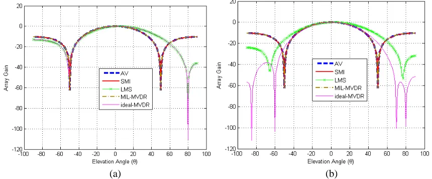
Figure 2. Array gain (dB) patterns of the beamformers at φ= 0◦,t= 100. (a) Left plot for Zone 1. (b) Right plot for Zone 4.
(a) (b)
Figure 3. Array gain (dB) patterns of the beamformers atφ= 0◦,t= 1000. (a) Left plot for Zone 1. (b) Right plot for Zone 4.
(a) (b)
Figure 4. MSE of the beamformers for the 7 interference zones and different number of antenna elements.
the FOM, a clear assessment on the beamformers performance is possible. Therefore, we conclude that the Array Pattern plots provide a first-cut assessment of the various beamformer’s performance while the MSE enables an in-depth assessment.
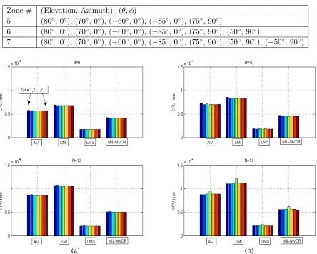
Table 3. Interference bearing setting for Zone 5 to 7.
Zone # (Elevation, Azimuth): (θ, φ)
5 (80◦, 0◦), (70◦, 0◦), (−60◦, 0◦), (−85◦, 0◦), (75◦, 90◦)
6 (80◦, 0◦), (70◦, 0◦), (−60◦, 0◦), (−85◦, 0◦), (75◦, 90◦), (50◦, 90◦)
7 (80◦, 0◦), (70◦, 0◦), (−60◦, 0◦), (−85◦, 0◦), (75◦, 90◦), (50◦, 90◦), (−50◦, 90◦)
(a) (b)
Figure 5. CPU time of the beamformers for the 7 interference zones and different number of antenna elements.
the LMS and a better MSE ratio of∼1/100 than the AV and SMI.
Finally, we compare the complexity of the four beamformers by computing the CPU time required to process one estimate ofw(.),Rˆ(.) and their associate functions used in the algorithms (see Section 3). The CPU time is an empirical result that relates to the computational complexity of the algorithm. Fig. 5 shows the CPU time for different N and interference zones. The results verify that the LMS algorithm has the lowest computational complexity while the SMI has the highest. Among the SAE-based algorithm (SMI, AV and MIL-MVDR), the MIL-MVDR has a lower complexity requirement than the SMI and the AV. The results also show that the number of antenna elements impact more on the complexity of the SAE-based algorithms than the LMS algorithm. On the other hand, the number of interference signals is less likely to impact the computational complexity of the algorithms.
5. CONCLUSIONS
scenarios with a high number of interference signals. In the converged phase, our proposed algorithm achieved lower MSE than the other three algorithms.
Next, we compare the nulling performance of the beamformers by looking at the Array Pattern and the array weight MSE. It demonstrated that the MSE is a better figure-of-merit for assessment of the beamformers in a multiple interference signals environment. For N = 8 to 14 antenna elements and up to 7 interference signals, the MIL-MVDR has shown to achieve the lowest converged MSE. The MIL-MVDR achieves a better MSE ratio of 1/1000 than the LMS and a better MSE ratio of 1/100 than the AV and SMI. We also evaluate the computational complexity of the beamforming algorithms and verify that the LMS has the lowest computational complexity (but at the expense of a higher MSE) while the MIL-MVDR is the next lower in complexity with its computational load about half that of the AV and SMI algorithms.
REFERENCES
1. Applebaum, S., “Adaptive arrays,”IEEE Trans. Antennas Propaga., Vol. 24, No. 5, 585–599, 1976. 2. Hudson, J. E.,Adaptive Array Principles, Peter Peregrinus Ltd-IET, 1981.
3. Brennan, L. E., J. D. Mallett, and I. S. Reed, “Adaptive arrays in airborne MTI radar,” IEEE Trans. Antennas Propaga., Vol. 24, 607–615, Sep. 1976.
4. Choi, S., J. Choi, H.-J. Im, and B. Choi, “A novel adaptive beamforming algorithm for antenna array CDMA systems with strong interferers,”IEEE Trans. Veh. Technol., Vol. 51, No. 5, 808–816, Sep. 2002.
5. Singh, H. and R. Jha, “Trends in adaptive array processing,”Int. J. Antennas Progpag., Vol. 2012, 2012.
6. Capon, J., “High-resolution Frequency-wavenumber spectrum analysis,” Proceedings of the IEEE, Vol. 57, No. 8, 1408–1418, 1969.
7. Haykin, S.,Adaptive Filter Theory, 4th Edition, Prentice Hall, New Jersey, 2002.
8. Vorobyov, S. A., “Principles of minimum variance robust adaptive beamforming design,” Elsevier Signal Processing, Vol. 93, No. 12, 3264–3277, Dec. 2013.
9. Liu, F., J. Wang, C. Y. Sun, and R. Du, “Robust MVDR beamformer for nulling level control via multi-parametric quadratic programming,” Progress In Electromagnetics Research C, Vol. 20, 239–254, 2011.
10. Reed, I. S., J. D. Mallett, and L. E. Brennan, “Rapid convergence rate in adaptive arrays,” IEEE Trans. Aerosp. Electron. Syst., Vol. 10, No. 6, 853–863, Nov. 1974.
11. Horowitz, L. L., H. Blatt, W. G. Brodsky, and D. K. Senne, “Controlling adaptive arrays with the sample matrix inversion algorithm,” IEEE Trans. Aerosp. Electron. Syst., Vol. 15, 840–847, Nov. 1979.
12. Hara, Y., “Weight-convergence analysis of adaptive antenna arrays based on SMI algorithm,”IEEE Trans. Wireless Communications, Vol. 2, No. 4, 749–757, July 2003.
13. Pados, D. A. and G. N. Karystinos, “An iterative algorithm for the computation of the MVDR filter,” IEEE Trans. Signal Process., Vol. 49, No. 2, 290–300, Feb. 2001.
14. Qian, H. and S. N. Batalama, “Data record-based criteria for the selection of an auxiliary vector estimator of the MMSE/MVDF filter,”IEEE Trans. on Commu., Vol. 51, No. 10, 1700–1708, Oct. 2003.
15. Seguin, E., R. Tessier, E. Knapp, and R. W. Jackson, “A dynamically reconfigurable phased array radar processing system,” Proc. Int. Conference on Field-Programmable Logic and Applications, 258–26, 20113.
16. Weedon, W. H., “Phased array digital beamforming hardware development at applied radar,”Proc. IEEE Int. Symp. Phased Array Systems and Technology, 854–859, 2010.
18. Wang, X., E. Aboutanios, M. Trinkle, and M. G. Amin, “Reconfigurable adaptive array beamforming by antenna selection,”IEEE Trans. Signal Process., Vol. 62, No. 9, May 2014. 19. Haupt, R. L., “Phase-only adaptive nulling with a genetic algorithm,” IEEE Trans. Antennas
Propaga., Vol. 45, 1009–1015, 1997.
20. Massa, A., M. Donelli, F. G. B. De Natale, S. Caorsi, and A. Lommi, “Planar antenna array control with Genetic algorithms and adaptive array theory,” IEEE Trans. Antennas Propaga., Vol. 52, 2919–2924, 2004.
21. Mahmoud, K. R., M. I. Eladawy, R. Bansal, S. H. Zainud-Deen, and S. M. M. Ibrahem, “Analysis of uniform circular arrays for adaptive beamforming applications using particle swarm optimization algorithm,” International Journal of RF and Microwave Computer-aided Engineering, Vol. 18, No. 1, 42–52, Jan. 2008.
22. Jakobsson, A., S. R. Alty, and S. Lambotharan, “On the implementation of the linearly constrained minimum variance beamformer,”IEEE Trans. Circuits Syst. II, Exp. Briefs, Vol. 53, No. 10, 1059– 1062, Oct. 2006.
23. Amin, M. and W. Sun, “A novel interference suppression scheme for global navigation satellite systems using antenna array,” IEEE J. Sel. Areas Commun., Vol. 23, No. 5, 999–1012, 2005. 24. Fante, R. L. and J. J. Vaccaro, “Wideband cancellation of interference in a GPS receive array,”
IEEE Trans. Aerosp. Electron. Syst., Vol. 36, No. 2, 549–564, Apr. 2000. 25. Balanis, C. A.,Antenna Theory, 2nd Edition, John Wiley, New Jersey, 1997.
26. Ong, L. T., “An adaptive beamformer based on adaptive covariance estimator,” Progress In Electromagnetics Research M, Vol. 36, 149–160, 2014.
27. Loecker, C., P. Knott, R. Sekora, and S. Algermissen, “Antenna design for a conformal antenna array demonstrator,”2012 6th European Conference on Antennas and Propagation (EUCAP), 151– 153, 2012.
28. Griffith, K. A. and I. J. Gupta, “Effect of mutual coupling on the performance of GPS AJ antennas,”