A Lightweight Robust Indoor Radio Tomographic Imaging Method
in Wireless Sensor Networks
Xiao Cao1, Hongchun Yao1, Yixian Ge2, and Wei Ke3, 4, *
Abstract—In recent years, radio tomographic imaging (RTI) is an emerging device-free localization (DFL) technology enabling the localization of people and other objects without requiring them to carry any electronic device. Different from other DFL techniques, the RTI method makes use of the changes of received signal strength (RSS) measured on links of the network to estimate the radio frequency (RF) attenuation field and forms an image of the changed field. This image is then used to infer the locations of targets within the deployed network. However, there still lacks an efficient scheme which can achieve robust location estimation performance with low computational cost. To solve this problem, we propose a lightweight robust RTI approach in this paper. The proposed method not only can reduce the algorithm’s storage and computational resource requirements, but also exploits the location information of wireless measurement nodes to improve the accuracy of the localization result, which ensures its robust performance. The effectiveness and robustness of the proposed scheme are demonstrated by experimental results where the proposed algorithm yields substantial improvement for localization performance and complexity.
1. INTRODUCTION
The proliferation of wireless communication and mobile computing has driven the demand of indoor location-based services (LBSs). Due to the low-cost advantage, a common approach to localization in wireless sensor networks (WSNs) is active RSS-based localization, wherein a radio device is attached to the target to be localized [1–5]. The target’s location is estimated by using RSS measurements between its radio device and other nodes in the network whose locations are known. However, in some applications such as battlefield surveillance, emergency rescue, and security safeguard, it is impractical to equip the target with a wireless device. Under these situations that conventional localization systems cannot be used, RSS-based DFL systems can infer the target’s location by measuring the target’s effect on the RSS of the network’s links. Therefore, RSS-based DFL without the need of carrying any device has recently become an attractive technology for determining an uncooperative target’s position [6, 7] Moreover, DFL techniques can also be used to reinforce existing device-dependent localization techniques to improve localization accuracy. In addition, compared with the existing device-free techniques such as infrared detector, video monitor and UWB radar detector, RSS-based DFL brings several advantages over other technologies by being able to work in obstructed environments, see through smoke, darkness, and walls, while avoiding the privacy concerns raised by video cameras.
As an emerging technique with promising application prospects, several RSS-based DFL approaches have been proposed in recent years. One significant approach of DFL is the fingerprint-based method,
Received 27 May 2017, Accepted 18 July 2017, Scheduled 28 August 2017
* Corresponding author: Wei Ke ([email protected]).
which matches the RSS samples collected online with the radio map constructed offline. Youssef et al. [7] originally adopted radio maps to store the RSS measurement of every link when the target is located at every possible location, and then matched the observed RSS to the training data for determining the target’s location. Then, the different fingerprint-based DFL method were further studied, e.g., in [8–10] under the same framework. Recently, Xiao et al. [11] made use of channel-state-information (CSI) to generalize the radio map, which provides a higher dimensional measurement per link which can then improve DFL performance. To investigate localization performance over time in a changing environment, Mager et al. [12] performed lots of experiments to quantify how changes in an environment affect accuracy, and proposed a correlation method for channel selection to help achieve a lower localization error rate even as the environment changes. The fingerprint-based method can well describe the relationship between link measurement and target location, but the training process is time consuming and labor intensive. Moreover, any significant change on the environment implies a costly new recalibration.
Another category of DFL is the geometric-based method. Instead of exploiting the offline training, the geometric-based method detects the wireless link line information affected by targets and uses simple operations on geometric objects to realize DFL. Geometric methods proposed in [13, 14] used a sensor-grid deployment and the overlap of shapes defined by shadowed links to estimate the target location. A disadvantage of the methods in [13, 14] is that no prior information about the target’s possible location is used to filter succeeding location estimates, making them sensitive to noise. To overcome this shortcoming, the geometric-filter (GF) method in [15] used a threshold value to detect the target-affected links, and then defined a circular prior region to remove outlying links and points. Finally, a location estimate was generated using the weighted mean of remaining points inside the circular prior region. However, the approach that treats the intersection points of shadowed links as probable target locations in the GF algorithm is a coarse approximation method. Moreover, the weight values are generated empirically, which may sometimes be unreasonable, and hence the performance of the GF algorithm based on the weighted mean method is not stable and particularly sensitive to the multipath fading effects.
Motivated by the success of the computed tomography method in medical and radar systems, references [16–18] formulated the DFL model as a radio tomography imaging problem. In [16], Wilson and Patwari introduced an elliptical model to describe the spatial impact area of a target on a wireless link, and then formed an image of the changed field by using the Tikhonov regularized method. The model assumes that the RSS of the link will change when a target is located inside the ellipse. The performance of RTI may be further improved with the assistance of frequency diversity [17], antenna diversity [18], power diversity [19] and compressive sensing [20–23]. Different from the elliptical model, Hamilton et al. [24] proposed a novel inverse area elliptical model (IAEM), which defines that the shadowing effect of a target on a wireless link is inversely proportional to the size of the smallest ellipse that contains the target. Recently, based on extensive experiments or the diffraction theory, the exponential-Rayleigh model (ERM) [25], diffraction model (DM) [26] and saddle surface model (SaS) [27] are proposed to model the RSS changes, and they are all incorporated into the particle filter framework to realize DFL.
Although these works significantly enrich the research of the RTI, one disadvantage of these methods is that all links in the WSN including the non-shadowed links are used to obtain the image of the attenuation field. In fact, many experiments have demonstrated that RSS is particularly sensitive to noise, and even the RSS measurements may still vary when the deployment area is vacant. Therefore, if these non-shadowed links are included to generate the image of the attenuation field, localization errors will become large because some spots that represent pseudotargets will also appear on the image. Meanwhile, more links will result in higher dimension of the matrix, so the inversion computation of high-dimensional matrix makes it difficult to be applied in some resource-constrained cases.
the RTI result, the low-complexity quasi-distance based localization method is proposed to improve the accuracy of the localization results.
The remainder of the paper is organized as follows. Section 2 describes the basic principle of RTI. The details of the adaptive threshold algorithm are addressed in Section 3. The LS-based optimization method is described in section 4. The experimental setup and experimental results are given in Section 5. Finally, Section 6 concludes the paper.
2. THE BASIC PRINCIPLE OF RTI
Suppose that the wireless network consists of M wireless nodes with known locations, and then the total number of wireless links with every pair of nodes is J = M ×(M −1)/2. Here, any pair of nodes is counted as a link, whether or not communication actually occurs between them. When wireless nodes communicate, the radio signals pass through the physical area of the network. Thus, the target’s presence inside the monitored region causes changes in the RSS of a subset of these J links due to scattering, reflection, diffraction or absorption. The shadowed links will be different when the target is located at different locations, and this makes it possible to realize DFL based on the link measurements. In RTI [16–18], the two-dimensional physical space is evenly divided into N pixels, and the corresponding image values at these pixels due to the presence of a target are denoted by x = [x1 x2 . . . xN]T. The work in [16] shows the efficacy of a linear model that relates the image x to
the RSS variations Y= [y1(t) y2(t) . . . yJ(t)]:
ΔY=Φx+n (1)
where yj(t) = abs[yj(t)−yj(0)] (j = 1,2, . . . , J) represents the change of the RSS measurement on jth link at timet; yj(t) is the vector of RSS measurements for jth link at time t;yj(0) is the baseline RSS measurement for jth link when the deployment area is vacant. n is a J ×1 noise vector, and Φ is a J×N matrix representing the weight of the target-affected contribution in each pixel on each link measurement. As shown in Fig. 1, the weighting of pixel ion linkj is formulated as [16]:
ϕji= 1 dj
1, if dji1+ dji2<dj+ρ
0, otherwise (2)
wheredji1 anddji2are the distances from the center of pixelito the two nodes of linkj,dj the distance
between two nodes of linkj, andρ a tunable parameter defining the width of the ellipse.
Once we have the forward model, the localization problem becomes an inverse problem: to estimate N dimensional position vectorxfromJ dimensional link measurement vectorY. However, this problem
Target Wireless Node
Weighted Pixel Zero-weight Pixel
dji1
dj
dji2
is an ill-posed inverse problem, since the same set of link measurements can lead to multiple different images when J < N. Therefore, regularization techniques such as Tikhonov regularization [16] and regularized least squares estimators [17] have been used. Here, we use the Tikhonov regularization approach, which is given as:
x=ΦTΦ+αQTQ−1ΦTΔY=ΠΔY (3)
whereQ is the Tikhonov matrix andα the regularization parameter. The linear transformation Π can be calculated beforehand enabling real-time image reconstruction.
3. LINK SELECTION BASED ON THE ADAPTIVE THRESHOLD METHOD
So far, most RTI methods exploit all J links to generate the image of the attenuation field, but the presence of the target only causes some links to be shadowed, and those links are affected depending on the current position of the target, as shown in Fig. 2. Once the non-shadowed links are included to calculate the inverse problem, the quality of the obtained image will be degraded, and some pseudo-targets’ spots will even appear on the image. Therefore, finding the affected links is essential for the RTI method.
Wireless Node
Target
Unaffected Link
Target-affected Link
Figure 2. Illustration of the target-affected links.
In fact, many experiments have demonstrated that a link may experience distinct attenuation or amplification due to the appearance of the target in its vicinity [15]. Therefore, if a link j can be considered to be shadowed by the target, its corresponding change in RSS measurement yj(t) must be above the shadowing detection threshold yth. To determine which links are shadowed by the target, in [15] a simple fixed threshold depending on the experiential value is used to detect the target-affected links, but this method ignores the time-varying factors on RSS measurements. In practice, RSS measurements are not only time-varying, but RSS measurements on the same links in the network may also significantly vary even if the deployment area is unchangeable. Therefore, using a single fixed threshold value may result in the misclassification of some links in real environments. To overcome this shortcoming, this paper proposes an adaptive threshold detection algorithm based on the fact that the RSS changes of the target-affected links may have higher value than the other unaffected links.
Firstly, letk= 0 and Δy(0)th be defined as the initial threshold value which can be chosen empirically, e.g., the median of Y. Then,J links are divided into two groups. Ifyj(t)>Δyth(0)(j= 1,2, . . . , J), then the link j belongs to group 1; otherwise, it is in group 2. Next, we calculate the mean of RSS changes in each group and obtain them from
μ1(k) =
1 J1
J1
j=1
Δyj(t) and μ2(k) =
1 J2
J2
j=1
whereJ1 andJ2 are the numbers of links in group 1 and 2, respectively. Correspondingly, the variance
of each group can be calculated as:
σ12(k) =
1 J1
J1
j=1
(Δyj(t)−μ1(k))2 and σ22(k) =
1 J2
J2
j=1
(Δyj(t)−μ2(k))2 (5)
In order to identify the target-affected group and unaffected group, two groups should have maximum difference under some appropriate threshold. Hence, we define the distance between two groups to denote this difference:
D(k)=
μ2(k)−Δyth(k) Δyth(k)−μ1(k)
(6)
At the same time, we hope that the variance of each group is small because the RSS changes in the same group have comparability. Therefore, combining these two considerations, we obtain the threshold selection parameter:
η(k)= D
(k)
σ21(k) +σ22(k)
(7)
Then, if Δymin < Δyth(k) < Δymax, let k= k+ 1, Δy(thk+1) = Δy(thk)±δ, and repeat the above process.
Δyminand Δymaxare the lower and upper limits of the threshold value, andδis the step length. Finally,
we choose the optimal threshold value Δyth∗ when the condition
η|Δy(k)
th=Δy∗th = max
D(k) σ2
1(k) +σ22(k)
, k= 1,2, . . .
(8)
is satisfied, and the corresponding links in group 1 are selected to generate the RTI estimate. Thus, not only negative effect of non-shadowed links is mitigated, but also the dimension of the model in Eq. (1) is reduced. For completeness, a full description of the adaptive threshold detection algorithm is given in Algorithm 1.
4. IMPROVING RTI RESULT BY USING NODE LOCATION INFORMATION
The above improved RTI method only uses RSS measurements of those links that are above the shadowing detection threshold to realize DFL, and thereby mitigating the noise influence and reducing the storage and computational requirements. Although non-shadowed wireless links are reduced by using the adaptive threshold method, not all of the detected effective links go through the vicinity of the target. Moreover, some experiments have found that the changes of RSS in some wireless links that are far from the target can also be above the shadowing detection threshold due to multipath effects. Therefore, the simple threshold method cannot eliminate the negative effect of all outlier links. In addition, the localization result from the RTI is only a approximation due to simply using the centroid of the target’s spot as the target position. Thus, the localization coordinaters= (xs, ys) obtained from RTI usually deviates from the true target location coordinate r0 = (x0, y0).
On the other hand, we find that in most DFL approaches wireless measurement nodes only take charge of communicating and measuring RSS values, but their location information is rarely utilized. In fact, the location information of wireless measurement nodes is not only known but usually accurate as well. This prior information can be utilized to improve the geometric localization result. Consequently, in this section we propose a quasi-distance based localization approach by using least squares (LS) optimization method to merge node location information into the DFL framework. Since the target still does not carry any device in the optimization step, we cannot measure the distances between the target and nodes by using the device-to-device method, which is different from the device-dependent distance-based localization. Therefore, we have to use the calculated distance through the RTI localization result and the coordinates of wireless nodes. Thus, not only the characteristic of DFL that does not carry any device is retained, but also accurate node location information is merged into DFL to improve localization performance.
According to the RTI localization coordinate rs = (xs, ys), the estimated distance between the coarse target location and lth wireless measurement node is
rl−rs=(xl−xs)2+ (y
l−ys)2 (9)
where rl = (xl , yl) represents the coordinates of the lth wireless measurement node, and • is the Euclidean norm. However, the true distance between the target location and the lth wireless measurement node is
rl−r0=
(xl−x0)2+ (yl−y0)2 (10)
Generally, there is a difference between the estimated and true distances which can be defined as
el = 1 2
rl−r02− rl−rs2
= −rTl r0+rTl rs+r02/2− rs2/2 (11)
where r0 =
x2
0+y02 and rs =
x2
s+y2s. Assume that L (L < M) nodes participate in the improved RTI process, so putting theL errors together and writing them in a vector form gives
e=Aθ−b (12)
where e= [e1 e2 . . . eL]T,θ= [x0 y0 R0]T,A=
⎡ ⎢ ⎢ ⎣
−x1 −y1 1/2 −x2 −y2 1/2
..
. ... ...
−xL −yL 1/2 ⎤ ⎥ ⎥ ⎦, b=
⎡ ⎢ ⎢ ⎣
Rs/2−x1xs−y1ys Rs/2−x2xs−y2ys
.. .
Rs/2−xLxs−yLys ⎤ ⎥ ⎥ ⎦,
R0 =r02 and Rs =rs2.
Naturally, we hope that the error vector ecan be reduced to zero. Hence, under the least squares (LS) criterion, the improved localization result can be obtained by
θ= (ATA)−1ATb (13)
systems, the networks in DFL consist of about twenty nodes. If all nodes are used to participate in the optimization-based DFL, it will result in high computational load, especially in the matrix inversion computation. In fact, lots of factors can be considered to determine which node is better to participate in the optimization, but in DFL we cannot obtain any information about the target except for RSS measurements. Since RSS measurement is particularly sensitive to noise, it is not a good indication to choose nodes. Therefore, we only consider the geometry effect of node configurations to select L nodes. Generally, three nodes that are not along the same straight line are enough for 2-D localization. However, since there is commonly the presence of measurement errors, more than three nodes are usually used to enhance the estimation accuracy under the LS localization framework, which is also the accustomed way in the device-dependent localization. According to the experimental results, we found that the location information of 4–6 noncollinear nodes was usually enough to improve the RTI result. Therefore, in most experiments, we chose only 4 nodes to participate in the optimization. Thus, the dimension of the model in Eq. (12) is not high, and the LS-based optimization method can obtain a good tradeoff between the tracking performance and computational complexity.
5. EXPERIMENTAL RESULTS
5.1. Physical Description of the Experiment
To demonstrate the applicability of the proposed method, we performed extensive experiments based on a prototype RTI system in two kinds of indoor environments. The wireless nodes use the 2.4 GHz IEEE 802.15.4 standard for communications, and the transceiver of each node is a system-on-chip (SoC) CC2530 device with a monopole antenna. Each node is about 0.9 m off the ground on a tripod in both environments. To avoid network transmission collisions, a simple token ring protocol is used to control transmission. Each node is assigned an ID number and programmed with a known order of transmission. When a node transmits, each node that receives the transmission examines the sender identification number and reserves the RSS from the transmitting node. The receiving nodes check to see if it is their turn to transmit, and if not, they wait for the next node to transmit. If one node does not transmit, or the packet is corrupted, a timeout causes each receiver to move to the next node in the schedule so that cycle is not halted. In our tests, it takes 5 ms for each node to broadcast a message, and it takes 140 ms for all the 28 nodes to perform one cycle of measurement. A base-station node listens to all broadcasts from the perimeter nodes and logs the RSS information to a mobile computer with 3.5 GHz processor and 8 GB memory for real-time processing.
To obtain the baseline RSS, measurements were taken for 60 s while the single human target is outside the deployment area. Afterwards, a target walked inside the deployment area along a predefined trajectory. In all experiments, we assume that the starting location of the target is known, which is generally used in many tracking algorithms [20]. To evaluate the performance of the improved RTI (iRTI) algorithm, we compare them with the traditional RTI algorithm and the geometric-based GF method under the same experimental conditions. The tracking error is defined as the distance between the known true target location and the estimated location obtained by each algorithm.
5.2. Performance Evaluation and Comparison
5.2.1. Localization Performance the Uncluttered Indoor Environment Scene 1)
(a) (b)
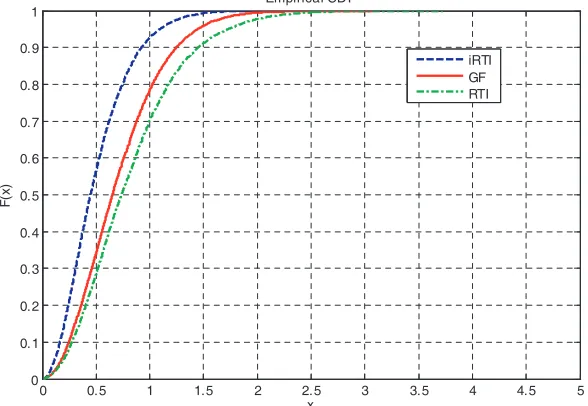
Figure 4. (a) Photograph of the experiment setup. (b) Geometry of the experiment setup.
0 0.5 1 1.5 2 2.5 3 3.5 4 4.5 5 0
0.1 0.2 0.3 0.4 0.5 0.6 0.7 0.8 0.9 1
x
F(
x
)
Empirical CDF
iRTI GF RTI
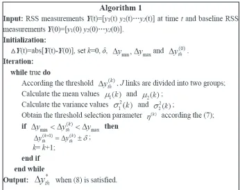
Figure 5. Cumulative distribution functions of the three algorithms in scene 1.
Figure 5 shows the error cumulative distribution functions (CDF) of the different algorithms in the uncluttered indoor environment. We can see that the proposed iRTI approach has the least tracking error. The proposed algorithm achieves the 90% location error at about 0.92 m, while the 90% location errors of the GF and RTI algorithms are around 125 m and 1.45 m, respectively. Especially, the iRTI algorithm is superior to the conventional RTI methods, which confirms the effectiveness of the proposed scheme by exploiting the location information of nodes and the adaptive threshold technique.
Table 1. Comparisons of tracking errors — Scene 1.
Algorithm Mean (m) Median (m) RMSE (m)
iRTI 0.376 0.444 0.321
iRTI without LS 0.479 0.610 0.383
GF 0.515 0.631 0.442
RTI 0.563 0.703 0.429
5.2.2. Localization Performance in the Highly Cluttered Indoor Environment (Scene 2)
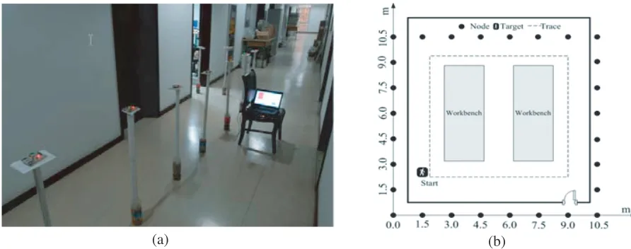
To evaluate the performance of the proposed method in rich multipath scenarios, an experiment was also conducted in a highly cluttered indoor environment inside a laboratory where there are numerous obstructions such as tables and other equipment. Moreover, only six nodes were placed inside the building, and other nodes were placed outside the brick wall. A photo and map of the experimental setup are shown in Figs. 6(a) and 6(b). In this scene, 28 nodes were deployed 1.5 m apart at the perimeter of a 10.5 m×10.5 m square area, and the number of pixels is 900. All other settings are similar to those in Scene 1.
(a) (b)
Figure 6. (a) Photograph of the experiment setup. (b) Geometry of the experiment setup.
0 1 2 3 4 5 6 0
0.1 0.2 0.3 0.4 0.5 0.6 0.7 0.8 0.9 1
x
F(
x
)
Empirical CDF
iRTI RTI GF
Figure 7. Cumulative distribution functions of the three algorithms in scene 2.
Table 2. Comparisons of tracking errors — Scene 2.
Algorithm Mean (m) Median (m) RMSE (m)
iRTI 0.728 1.011 0.858
iRTI without LS 0.963 1.444 1.077
GF 1.379 1.899 1.912
RTI 1.195 1.626 1.309
5.2.3. Discussion
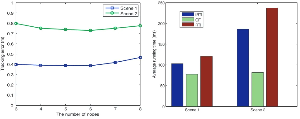
In this subsection, we evaluate the proposed iRTI scheme under different parameters to analyse its performance. Fig. 8 illustrates the tracking performance with different numbers of nodes in the LS-based optimization process for iRTI. It is observed from Fig. 8 that the improvement of tracking errors is not conspicuous with the increase in the number of nodes, and even the accuracy decreases slightly when the number of nodes increases to seven or higher. This means that the location information of 4–6 noncollinear nodes is enough to improve the localization result, which can help to have a good tradeoff between the tracking performance and computational complexity.
3 4 5 6 7 8 0 0.1 0.2 0.3 0.4 0.5 0.6 0.7 0.8 0.9 1
The number of nodes
Tr ac k ing e rr o r ( m ) Scene 1 Scene 2
Figure 8. Effects of the different number of nodes that take part in the LS-based process.
Scene 1 Scene 2 0 50 100 150 200 250 A v er age r u nn in g t im e ( m s ) iRTI GF RTI
Figure 9. Running times of different algorithms.
6. CONCLUSION
The appeal of using DFL systems is its applicability in situations in which conventional localization systems cannot be used. As an important type of DFL, RTI plays an increasingly important role in many applications ranging from intrusion detection to elder care. In order to enhance tracking performance and keep low computing complexity, this paper proposes an improved RTI method. To overcome the negative effect of non-shadowed links, an adaptive threshold detection algorithm is proposed to find the target-affected links. Thus, the iRTI method can not only solve the problem of outlier links, but also reduce the algorithm’s storage and computational resource requirements. In the LS-based optimization process, the location information of wireless nodes is exploited as an assisted condition to enhance the RTI accuracy. To the best of our knowledge, node location information is first merged into RTI to improve localization performance. The effectiveness of the proposed scheme has been demonstrated by experimental results in two kinds of indoor environments where substantial improvement for localization performance is achieved.
In our future work, we will try to explore how to realize multi-target localization. Meanwhile, for the proposed scheme we will consider the theoretic bound on the location estimation precision.
ACKNOWLEDGMENT
This work was supported by the Science and Technology Program of SGCC (NY71-16-034), the Priority Academic Program Development of Jiangsu Higher Education Institutions (PAPD), the Specialized Research Fund for the Doctoral Program of Higher Education of China (Grant No. 20133207120007) and the Open Research Fund of Jiangsu Key Laboratory of Meteorological Observation and Information Processing (Grant No. KDXS1408).
REFERENCES
1. Gezici, S., “A survey on wireless position estimation,”Wireless Personal Communications, Vol. 44, No. 3, 263–282, 2008.
3. He, S. N. and S. H. G. Chan, “Wi-Fi fingerprint-based indoor positioning: Recent advances and comparisons,” IEEE Trans. Surv. Tutor., Vol. 18, No. 1, 466–490, 2016.
4. Guvenc, I. and C. C. Chong, “A survey on TOA based wireless localization and NLOS mitigation techniques,” IEEE Commun. Surveys& Tutorials, Vol. 11, 107–124, 2009.
5. Liu, H., H. Darabi, H. Banerjee, and J. Liu, “Survey of wireless indoor positioning techniques and systems,”IEEE Trans. Systems, Man, and Cybernetics — Part C, Vol. 37, No.‘6, 1067–1080, 2007. 6. Patwari, N. and J. Wilson, “RF sensor networks for device-free localization: Measurements, models,
and algorithms,” Proc. of the IEEE, Vol. 98, No. 11, 1961–1973, 2010.
7. Youssef, M., M. Mah, and A. Agrawala, “Challenges: Device-free passive localization for wireless environments,”13th ACM MobiCom, 222–229, 2007.
8. Seifeldin, M., A. Saeed, A. Kosba, A. El-keyi, and M. Youssef, “Nuzzer: A large-scale device-free passive localization system for wireless environments,”IEEE Trans. Mob. Comput., Vol. 12, No. 7, 1321–1334, 2013.
9. Saeed, A., A. Kosba, and M. Youssef, “Ichnaea: A low-overhead robust WLAN device-free passive localization system,” IEEE J. Sel. Topics Signal Process., Vol. 8, No. 1, 5–15, 2014.
10. Sabek, I., M. Youssef, and A. V. Vasilakos, “ACE: An accurate and efficient multi-entity device-Free WLAN localization system,” IEEE Trans. Mob. Comput., Vol. 14, No. 2, 261–273, 2015.
11. Xiao, J., K. Wu, Y. Yi, L. Wang, and L. M. Ni, “Pilot: Passive device-free indoor localization using channel state information,” Proc. 33th Int. Conf. Distrib. Comput. Syst., 236–245, 2013. 12. Mager, B., P. Lundrigan, and N. Patwari, “Fingerprint-based device-free localization performance
in changing environments,” IEEE J. Sel. Areas Commun., Vol. 33, No. 11, 2429–2438, 2015. 13. Zhang, D., J. Ma, Q. Chen, and L. Ni, “An RF-based system for tracking transceiver-free objects,”
Proc. Fifth Annual IEEE International Conference on Pervasive Computing and Communications, 135–144, 2007.
14. Zhang, D., K. Lu, R. Mao, R. Y. Feng, Y. Liu, Z. Ming, and L. Ni, “Fine-grained localization for multiple transceiver-free objects by using RF-based technologies,” IEEE Trans. Parallel Distrib. Syst. Vol. 25, No. 6, 1464–1475, 2014.
15. Talampas, M. C. R. and K. S. Low, “A geometric filter algorithm for robust device-free localization in wireless networks,” IEEE Trans. Ind. Informat., Vol. 12, No. 5, 1670–1678, 2016.
16. Wilson, J. and N. Patwari, “Radio tomographic imaging with wireless networks,” IEEE Trans. Mob. Comput., Vol. 9, No. 5, 621–632, 2010.
17. Kaltiokallio, O., M. Bocca, and N. Patwari, “Enhancing the accuracy of radio tomographic imaging using channel diversity,” Proc. 9th IEEE Int. Conf. MASS, 254-262, 2012.
18. Bocca, M., A. Luong, N. Patwari, and T. Schmid, “Dial it in: Rotating RF sensors to enhance radio tomography,” arXiv, 2013, [Online], Available: http://arxiv.org/abs/1312.5480.
19. Wang, J., Q. Gao, H. Wang, P. Cheng, and K. Xin, “Device-free localization with multi-dimensional wireless link information,” IEEE Trans. Veh. Technol., Vol. 64, No. 1, 356–366, 2015.
20. Yang, Z. Y., K. D. Huang, X. M. Guo, and G. L. Wang, “A real-time device-free localization system using correlated RSS measurements,” EURASIP J. Wireless Commu. Netw., Vol. 2013, No. 186, 1–12, 2013.
21. Wang, J., Q. Gao, X. Zhang, and H. Wang, “Device-free localization with wireless networks based on compressing sensing,” IET Commun., Vol. 6, No. 15, 2395–2403, 2012.
22. Kanso, M. A. and M. G. Rabbat, “Compressed RF tomography for wireless sensor networks: centralized and decentralized approaches,” Proc. 5th DCOSS, 173–186, 2009.
23. Ke, W., G. Liu, and T. Fu, “Robust sparsity-based device-free passive localization in wireless networks,” Progress In Electromagnetics Research C, Vol. 46, 63–73, 2014.
25. Guo, Y., K. Huang, N. Jiang, X. Guo, and G. Wang, “An exponential-Rayleigh model for RSS-based device-free localization and tracking,”IEEE Trans. Mob. Comput., Vol. 14, No. 3, 484–494, 2015.
26. Wang, Z. H., H. Liu, S. X. Xu, X. Y. Bu, and J. P. An, “A diffraction measurement model and particle filter tracking method for RSS-based DFL,”IEEE J. Sel. Areas Commun., Vol. 33, No. 11, 2391–2403, 2015.