Study of UPML Absorbing Boundary Condition for the Five-Step
LOD-FDTD Method
Lixia Yang1, *, Xuejian Feng1, and Lunjin Chen2
Abstract—In this paper, the uniaxial anisotropic perfectly matched layer (UPML) absorbing boundary condition in unconditionally stable five-step locally one-dimensional finite-difference time-domain (LOD5-FDTD) method is deduced. The UPML absorbing boundary condition (ABC) is validated based on comparison with a simulation in larger domain (and thus without reflection) in the first test. Then using a sinusoidal source, target field phase distribution surrounded by the UPML-ABC is analyzed. The results further illustrate the stability and efficiency of the UPML absorbing boundary condition.
1. INTRODUCTION
The three-dimensional five-step LOD-FDTD (LOD5-FDTD) method [1] is an unconditionally stable method whose time step is not restricted by the Courant-Friedrich-Lewy (CFL) stability condition [2]. It is worth mentioning that the LOD5-FDTD method has second-order accuracy in time domain and yields less numerical dispersion than the ADI-FDTD [3, 4], two-step LOD-FDTD [5], and three-step LOD-FDTD [6] methods.
For application to the simulation of the electromagnetic scattering and propagation in the free-space, the LOD-FDTD method should have an efficient absorbing layer in the computation field. In [7, 8], the split-field perfectly matched layer (PML) and convolution PML have been applied to LOD-FDTD method. And the Mur’s and uniaxial anisotropic PML (UPML) absorbing boundary condition [9–12] have been implemented within the two-dimensional LOD-FDTD method [13]. More recently, there are some other PML-ABC applied in the LOD-FDTD method such as LOD-CPML [14] and LOD-SC-PML [15]. In this paper, the ULOD-SC-PML-ABC is applied to the LOD5-FDTD method. Using the proposed UPML-ABC, the reflection error of an electric dipole source and target field phase distribution of a sinusoidal source are computed. The results of these simulation experiments show that the UPML-ABC can be used efficiently in the LOD5-FDTD method.
2. FORMULATION
In the UPML medium, the Maxwell’s curl equations in frequency domain can be written as follows [9]
∇ ×H⃗ = jωε0εrε ⃗¯¯E (1)
∇ ×E⃗ = −jωµ0µrµ ⃗¯¯H (2)
where εr and µr are the relative permittivity and permeability of the isotropic space, and ¯ε, ¯¯ µ¯ are
relative permittivity and permeability tensors, respectively, which can be written as
¯ ¯ ε= ¯µ¯ =
sysz
sx 0 0
0 sxsz
sy 0
0 0 sxsy sz
, sQ=κQ+
σQ
jωε0
, Q=x, y, z (3)
Received 23 February 2016, Accepted 24 March 2016, Scheduled 13 April 2016
* Corresponding author: Lixia Yang ([email protected]).
1 Department of Communication Engineering, Jiangsu University, Zhenjiang, China. 2Department of Physics, University of Texas
whereκQ and σQ are the attenuation factor and conductivity, respectively.
For the traditional LOD5-FDTD method, first sub-step equations are written as follow [1]
Eyn+1/6 = Eny −∆t 4ε
(
∂Hzn ∂x +
∂Hzn+1/6
∂x
)
(4)
Ezn+1/6 = Enz +∆t 4ε
(
∂Hyn ∂x +
∂Hyn+1/6
∂x
)
(5)
Hyn+1/6 = Hyn+ ∆t 4µ
(
∂Ezn ∂x +
∂Ezn+1/6
∂x
)
(6)
Hzn+1/6 = Hzn− ∆t 4µ
(
∂Eyn ∂x +
∂Eyn+1/6
∂x
)
(7)
Equations (4)–(7) can be transformed as follows
−2ε1
3 ∂Ey
∂t = ∂Hzn
∂x +
∂Hzn+1/6
∂x (8)
2ε1
3 ∂Ez
∂t = ∂Hn
y
∂x +
∂Hyn+1/6
∂x (9)
2µ1
3 ∂Hy
∂t = ∂Ezn
∂x +
∂Ezn+1/6
∂x (10)
−2µ1
3 ∂Hz
∂t = ∂Eyn
∂x +
∂Eyn+1/6
∂x (11)
Then Equations (8)–(11) transform into frequency domain are written as follows
−2
3jωε1 ∂Ey
∂t = ∂Hzn
∂x +
∂Hzn+1/6
∂x (12)
2 3jωε1
∂Ez
∂t = ∂Hyn
∂x +
∂Hyn+1/6
∂x (13)
2 3jωµ1
∂Hy
∂t = ∂Ezn
∂x +
∂Ezn+1/6
∂x (14)
−2
3jωµ1 ∂Hz
∂t = ∂Eyn
∂x +
∂Eyn+1/6
∂x (15)
Then for the UPML medium, the LOD5-FDTD method equations in frequency domain can be written as follows
First sub-step
−2
3jωε1 sxsz
sy
Ey =
∂Hzn ∂x +
∂Hzn+1/6
∂x (16)
2 3jωε1
sxsy
sz
Ez =
∂Hyn ∂x +
∂Hyn+1/6
∂x (17)
2 3jωµ1
sxsz
sy
Hy =
∂Ezn ∂x +
∂Ezn+1/6
∂x (18)
−2
3jωµ1 sxsy
sz
Hz =
∂Eyn ∂x +
∂Eyn+1/6
Second sub-step
2 3jωε1
sysz
sx
Ex =
∂Hzn+1/6
∂y +
∂Hzn+2/6
∂y (20)
−2
3jωε1 sxsy
sz
Ez =
∂Hxn+1/6
∂y +
∂Hxn+2/6
∂y (21)
−2
3jωµ1 sysz
sx
Hx =
∂Ezn+1/6
∂y +
∂Ezn+2/6
∂y (22)
2 3jωµ1
sxsy
sz
Hz =
∂Exn+1/6
∂y +
∂Exn+2/6
∂y (23)
Third sub-step
−2
3jωε1 sysz
sx
Ex =
∂Hyn+2/6
∂z +
∂Hyn+4/6
∂z (24)
2 3jωε1
sxsz
sy
Ey =
∂Hxn+2/6
∂z +
∂Hxn+4/6
∂z (25)
2 3jωµ1
sysz
sx
Hx =
∂Eyn+2/6
∂z +
∂Eyn+4/6
∂z (26)
−2
3jωµ1 sxsz
sy
Hy =
∂Exn+2/6
∂z +
∂Exn+4/6
∂z (27)
Fourth sub-step
2 3jωε1
sysz
sx
Ex =
∂Hzn+4/6
∂y +
∂Hzn+5/6
∂y (28)
−2
3jωε1 sxsy
sz
Ez =
∂Hxn+4/6
∂y +
∂Hxn+5/6
∂y (29)
−2
3jωµ1 sysz
sx
Hx =
∂Ezn+4/6
∂y +
∂Ezn+5/6
∂y (30)
2 3jωµ1
sxsy
sz
Hz =
∂Exn+4/6
∂y +
∂Exn+5/6
∂y (31)
Fifth sub-step
−2
3jωε1 sxsz
sy
Ey =
∂Hzn+5/6
∂x +
∂Hn+1 z
∂x (32)
2 3jωε1
sxsy
sz
Ez =
∂Hyn+5/6
∂x +
∂Hn+1 y
∂x (33)
2 3jωµ1
sxsz
sy
Hy =
∂Ezn+5/6
∂x +
∂En+1 z
∂x (34)
−2
3jωµ1 sxsy
sz
Hz =
∂Eyn+5/6
∂x +
∂En+1 y
∂x (35)
whereε1 =ε0εr,µ1 =µ0µr. The following six auxiliary variables are defined:
Dx =
2 3ε1
sz
sx
Ex, Dy =
2 3ε1
sx
sy
Ey, Dz =
2 3ε1
sy
sz
Ez (36)
Bx =
2 3µ1
sz
sx
Hx, By =
2 3µ1
sx
sy
Hy, Bz =
2 3µ1
sy
sz
Take the first sub-step as an example by substituting Eqs. (36), (37) into Eqs. (16)–(19) and converting the expression from frequency domain to time domain with the aid ofjω→∂/∂t, we obtain the expression for the first sub-step of the five sub-steps:
∂Ezn ∂x +
∂Ezn+1/6
∂x = 2 3
∂
∂t(szBy) (38)
∂Eyn ∂x +
∂Eyn+1/6
∂x = 2 3
∂
∂t(−sxBz) (39) ∂Hzn
∂x +
∂Hzn+1/6
∂x = 2 3
∂
∂t(−szDy) (40) ∂Hyn
∂x +
∂Hyn+1/6
∂x = 2 3
∂
∂t(sxDz) (41)
Due to implicit nature of the LOD5-FDTD UPML in Eqs. (38)–(41), in their current form, it is computationally expensive to simulate. Therefore, for efficient simulation, these equations are further simplified. By using central difference scheme for time and spatial derivative, we can solve the electric and magnetic field components of the UPML. Here, electric field componentEyn+1/6 is shown as follows
after putting Eq. (40) into Eq. (39):
aEyn(+1i−/16,j+1/2,k)+bEyn(+1i,j/+16/2,k)+cEyn(+1i+1/6,j+1/2,k)=d (42)
where:
a = −9 4
1
µ1ε1(∆x)2
1
AAX(i, j+ 1/2, k)
1
AAX(i−1/2, j+ 1/2, k)
b = 1 +9 4
1
µ1ε1(∆x)2 (
1
AAX(i, j+ 1/2, k)
1
AAX(i+ 1/2, j+ 1/2, k)
+ 1
AAX(i, j+ 1/2, k)
1
AAX(i−1/2, j+ 1/2, k)
)
c = −9 4
1 µ1ε1(∆x)2
1
AAX(i, j+ 1/2, k)
1
AAX(i+ 1/2, j+ 1/2, k)
AAX = 6κx
∆t + σx
2ε0
, AAY= 6κy ∆t +
σy
2ε0
AAZ = 6κz
∆t + σz
2ε0
, BBX= 6κx ∆t −
σx
2ε0
BBY = 6κy
∆t − σy
2ε0
, BBZ= 6κz ∆t −
σz
2ε0
Since electric componentEyn+1/6 is already known, auxiliary variable Bzn+1/6 can be updated with Eq.
(38). Then, magnetic component Hzn+1/6 can be updated with the third formula of Eq. (37).
Hzn(+1i+1/6/2,j+1/2,k) = eHzn(i+1/2,j+1/2,k)+f Bzn(i+1/2,j+1/2,k)
+g
(
Eyn(+1i+1/6,j+1/2,k)−Eyn(+1i,j/+16/2,k)+Eyn(i+1,j+1/2,k)−Eyn(i,j+1/2,k)
)
(43)
where:
e = BBY(i+ 1/2, j+ 1/2, k)
AAY(i+ 1/2, j+ 1/2, k)
f = AAZ(i+ 1/2, j+ 1/2, k) µ1AAY(i+ 1/2, j+ 1/2, k)
BBX(i+ 1/2, j+ 1/2, k)
AAX(i+ 1/2, j+ 1/2, k) −
BBZ(i+ 1/2, j+ 1/2, k) µ1AAY(i+ 1/2, j+ 1/2, k)
g = −3 2
1
∆x·AAX(i+ 1/2, j+ 1/2, k)
Similar to Eqs. (38)–(43), for the other four sub-steps, the updating electric and magnetic field components can also be derived.
d=
{
BBX(i, j+ 1/2, k)
AAX(i, j+ 1/2, k) − 9 4
1 µ1ε1(∆x)2
·
( 1
AAX(i,j+1/2,k)AAX(i+1/2,j+1/2,k)
+AAX(i,j+1/2,k)AAX1 (i−1/2,j+1/2,k)
)}
Eyn(i,j+1/2,k)
−1
ε1 (
BBY(i, j+ 1/2, k)
AAX(i, j+ 1/2, k)−
AAY(i, j+ 1/2, k)BBZ(i, j+ 1/2, k)
AAX(i, j+ 1/2, k)AAZ(i, j+ 1/2, k)
)
Dyn(i,j+1/2,k)
−3
2 1 ε1∆x
AAY(i, j+ 1/2, k)
AAX(i, j+ 1/2, k)AAZ(i, j+ 1/2, k) ·
{(
1 +BBY(i+ 1/2, j+ 1/2, k)
AAY(i+ 1/2, j+ 1/2, k)
)
Hzn(i+1/2,j+1/2,k)−
(
1 +BBY(i−1/2, j+ 1/2, k)
AAY(i−1/2, j+ 1/2, k)
)
Hzn(i−1/2,j+1/2,k)
}
+9 4
1 µ1ε1(∆x)2
1
AAX(i, j+ 1/2, k) ·
(
1
AAX(i+ 1/2, j+ 1/2, k)E
n
y(i+1,j+1/2,k)
+ 1
AAX(i−1/2, j+ 1/2, k)E
n
y(i−1,j+1/2,k) )
− 3
2 1 µ1ε1∆x
AAY(i, j+ 1/2, k)
AAX(i, j+ 1/2, k)AAZ(i, j+ 1/2, k)
·
{(
AAZ (i+1/2, j+1/2, k)BBX(i+1/2, j+1/2, k)
AAY(i+1/2, j+1/2, k)AAX(i+1/2, j+1/2, k)−
BBZ(i+1/2, j+1/2, k)
AAY(i+1/2, j+1/2, k)
)
Bzn(i+1/2,j+1/2,k)
−
(
AAZ(i−1/2, j+1/2, k)BBX(i−1/2, j+1/2, k)
AAY(i−1/2, j+1/2, k)AAX(i−1/2, j+1/2, k)−
BBZ(i−1/2, j+1/2, k)
AAY(i−1/2, j+1/2, k)
)
Bzn(i−1/2,j+1/2,k)
}
3. NUMERICAL RESULTS
In this section, we use two numerical simulation tests to validate the proposed methods.
In the first test, a point electric dipole source is located at the center of the computation region. A Gaussian pulse P(t) = 10−10exp[−((t−3T)/T)2], with T = 2 ns, is used as the excitation source. The structure of the computation region has 40×40 ×40 cells, with 40 cells along each of x, y, and z directions, and the UPML has 10 cells along x, y and z directions. The spatial step is set as ∆x= ∆y = ∆z= 5 cm.
For the purpose of comparison, a reference solution without UPML-ABC is computed by using a larger domain (160×160×160 cells). The relative reflection error is defined as:
δ= 20 log10
(
|Ez−Eref|
max|Eref| )
(44)
whereEref is electric field at the same observation point for a lager domain without reflection.
CFL number (S) is defined as the ratio of the time step size (∆t) to the CFL limit (∆tCF L =
∆x/√3/c):
CF LN = ∆t ∆tCF L
(45)
And the UPML-ABC parameters for implicit LOD5-FDTD method are given as:
σmax= 0.9σopt, κmax= 10 (46)
where σopt were given in [9], σopt = (m+ 1)/(150π∆x√εr), and m is the order of polynomial scaling.
Take xdirection as an example,
σx(x) = (x/d)mσx,max (47)
κx(x) = 1 + (κx,max−1)·(x/d)m (48)
where dis the depth of the UPML. The value ofσx starts with 0 at x= 0 (the surface of the UPML)
and increases toσx,max atx=d(the PEC outer boundary) in the UPML. Similarly, for the UPML,κx
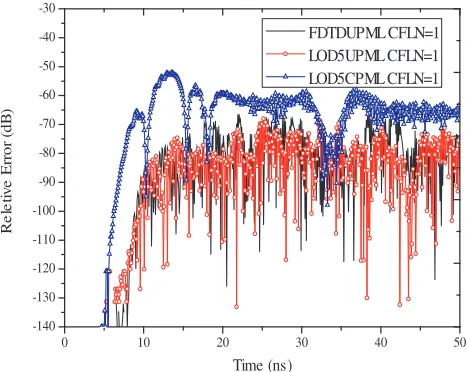
Figure 1 shows the relative error of the three methods observed at CFLN = 1. Fig. 1 demonstrates that both LOD5UPML and conventional FDTDUPML have almost the same relative error and nearly
−15 dB smaller than the LOD5CPML method on average. For further analysis of the method, Figs. 2–5 show relative error with respect to time for different CFLNs at different observation points. Fig. 2 shows the relative errors with different values of CFLN (= 1,4, and 9) at the observation pointEz(0,10∆y,0)
for LOD5CPML. Fig. 3 shows the relative errors with different values of CFLN (= 1,4, and 9) at the observation point Ez(0,10∆y,0) for LOD5UPML. Fig. 4 shows the relative errors with different
values of CFLN (= 1,4, and 9) at the observation point Ez(10∆x,10∆y,0) for LOD5UPML. And
Fig. 5 shows the relative errors with different values of CFLN (= 1,4, and 9) at the observation point Ez(0,10∆y,0) for LOD5CPML. Fig. 3 shows the relative errors with different values of CFLN (= 1,4,
and 9) at the observation point Ez(0,10∆y,0) for LOD5UPML. Fig. 4 shows the relative errors with
different values of CFLN (= 1,4, and 9) at the observation point Ez(10∆x,10∆y,0) for LOD5UPML.
0 10 20 30 40 50
-140 -130 -120 -110 -100 -90 -80 -70 -60 -50 -40 -30
R
e
le
ti
v
e
E
rr
or
(
dB
)
Time (ns)
FDTDUPML CFLN=1 LOD5UPML CFLN=1 LOD5CPML CFLN=1
Figure 1. Relative error of the LOD5-FDTD UPML, CPML and conventional FDTD UPML for CFLN = 1 at pointEz(0,10∆y,0).
0 10 20 30 40 50
-140 -130 -120 -110 -100 -90 -80 -70 -60 -50 -40 -30
R
e
le
ti
v
e
E
rr
or
(
dB
)
Time (ns)
LOD5CPML CFLN=1 LOD5CPML CFLN=4 LOD5CPML CFLN=9
Figure 2. The relative error against time at the observation pointEz(0,10∆y,0) for LOD5CPML.
0 10 20 30 40 50
-140 -130 -120 -110 -100 -90 -80 -70 -60 -50 -40 -30
R
e
la
ti
v
e
E
rr
or
(
dB
)
Time (ns)
LOD5UPML CFLN=1 LOD5UPML CFLN=4 LOD5UPML CFLN=9
Figure 3. The relative error against time at the observation point Ez(0,10∆y,0) for
LOD5UPML.
0 10 20 30 40 50
-140 -130 -120 -110 -100 -90 -80 -70 -60 -50 -40 -30
LOD5UPML CFLN=1 LOD5UPML CFLN=4 LOD5UPML CFLN=9
R
e
la
ti
v
e
E
rr
or
(
dB
)
Time (ns)
Figure 4. The relative error against time at the observation point Ez(10∆x,10∆y,0) for
And Fig. 5 shows the relative errors with different values of CFLN (= 1,4, and 9) at the observation point Ez(10∆x,10∆y,10∆z) for LOD5UPML. From Fig. 2 it can be observed that the reflection error
is below −35 dB for any CFLN bellow 9 for LOD5CPML. From Fig. 3 and Fig. 4, it can be observed that the reflection error is well below −50 dB for any CFLN bellow 9 for LOD5UPML. And it can be observed from Fig. 5 for any S bellow 9 that the reflection error is well below the maximum value
−48 dB for LOD5UPML. Comparing Fig. 2 with Fig. 3, it can also be observed that the relative error of the LOD5UPML is nearly −15 dB smaller than the LOD5CPML on average when CFLN = 1,4,9 at the observation point Ez(0,10∆y,0). The refection error performance of all the three observation
points illustrates that the proposed UPML-ABC has good absorption effect.
For the second test, target field phase distribution of a sinusoidal source is analyzed with UPML-ABC. The computation region has 160×160×160 cells. And the computation region is surrounded by additional 10-cell UPML absorbing layers. Excitation source expression is as follows:
P(t) = ˆezsin(ωt), ω= 2πf (49)
where f = 3 GHz and LOD5-FDTD cell size is ∆x = ∆y = ∆z = 5 cm. Fig. 6 shows the radiation
0 10 20 30 40 50
-140 -130 -120 -110 -100 -90 -80 -70 -60 -50 -40 -30
R
e
la
ti
v
e
E
rr
or
(
dB
)
Time (ns)
LOD5UPML CFLN=1 LOD5UPML CFLN=4 LOD5UPML CFLN=9
Figure 5. The relative error against time at the observation point Ez(10∆x,10∆y,10∆z) for
LOD5UPML.
-80 -60 -40 -20 0 20 40 60 80
-80 -60 -40 -20 0 20 40 60 80
X / dx
Y /
d
y
-3 -2 -1 0 1 2 3
Figure 6. The radiation phase distribution ofEz
atz= 0 plane with source at (0,0,0).
-80 -60 -40 -20 0 20 40 60 80
-80 -60 -40 -20 0 20 40 60 80
X / dx
Y /
d
y
-3 -2 -1 0 1 2 3
Figure 7. The radiation phase distribution ofEz
phase distribution ofEz component at thexoy plane when the sinusoidal source is located at the center
point (0,0,0), and Fig. 7 shows the radiation phase distribution of theEz component at thexoy plane
when the sinusoidal source is located at the center point (60,60,60). The CFL number CFLN is set to 4.0. No clear distortion of phase distribution in the computation domain is seen, demonstrating efficient absorbing performance for LOD5-FDTD UPML method.
4. CONCLUSIONS
In this paper, the uniaxial anisotropic perfectly matched layer (UPML) absorbing boundary condition (ABC) in unconditionally stable five-step locally one-dimensional finite-difference time-domain (LOD5-FDTD) method is presented. Relative errors are analyzed at different CFLN conditions. The relative error of the proposed method is compared with the conventional FDTD method and CPML method at CFLN = 1. The result shows good agreement with the conventional FDTD method and nearly
−15 dB smaller than the CPML method on average. Comparing Fig. 2 with Fig. 3, it can also be observed that the relative error of the proposed method is still nearly −15 dB smaller than the CPML method on average when CFLN = 4,9 at the observation point Ez(0,10∆y,0). The refection error
performance of all the three observation points illustrates that the proposed UPML-ABC has good absorption effect. However, the advantage of the LOD-FDTD UPML is its applicability at higher CFLN. To further validate the stability and absorption efficiency of the proposed method, the radiation phase distribution of a sinusoidal source is studied. No clear distortion of phase distribution in the computation domain is seen, demonstrating efficient absorbing performance for the propose UPML method. This development of UPML for the three-dimensional LOD5-FDTD method will enhance applications of the FDTD method.
ACKNOWLEDGMENT
This work is supported by the National Natural Science Foundation of China under Grant (No. 61072002), Elitist of Liu-Da Summit Project in Jiangsu Province at 2011 under Grant (No. 2011-DZXX-031), and graduate research innovation (KYXX 0034). LC acknowledges the support of NSF grant AGS-1405041.
REFERENCES
1. Saxena, A. K. and K. V. Srivastava, “A three-dimensional unconditionally stable five-step LOD-FDTD method,”IEEE Trans. Antenna Propag., Vol. 62, No. 3, 1321–1329, Mar. 2014.
2. Courant, R., K. Friedrichs, and H. Lewy, “On the partial difference equations of mathematical physics,”IBMJ, Vol. 11, 215–234, Mar. 1967.
3. Namiki, T., “A new FDTD algorithm based on alternating-direction implicit method,”IEEE Trans.
Microw. Theory. Tech., Vol. 47, No. 10, 2003–2007, Oct. 1999.
4. Zheng, F., Z. Chen, and J. Zhang, “A finite-difference time-domain method without the Courant stability conditions,” IEEE Microw. Guided Wave Lett., Vol. 9, No. 11, 441–443, Nov. 1999. 5. Tan, E. L., “Unconditionally stable LOD-FDTD method for 3-D Maxwell’s equations,” IEEE
Microwave and Wireless Components Letters, Vol. 17, No. 2, 85–87, Feb. 2007.
6. Ahmed, I., E. K. Chua, E. P. Li, and Z. Chen, “Development of the three dimensional unconditionally stable LOD-FDTD method,”IEEE Trans. Antenna Propag., Vol. 56, No. 11, 3596– 3600, Nov. 2008.
7. Do Nascimento, V. E., B. H. V. Borges, and F. L. Teixeira, “Split-field PML implementations for the unconditionally stable LOD-FDTD method,” IEEE Microwave and Wireless Components
Letters, Vol. 16, No. 7, 398–400, Jul. 2006.
9. Gedney, S. D., “An Anisotropic perfectly matched layer-absorbing medium for the truncation of FDTD lattices,”IEEE Trans. Antenna Propag., Vol. 44, No. 12, 1630–1639, Dec. 1996.
10. Sun, W., N. G. Loeb, and Q. Fu, “Finite-difference time domain solution of light scattering and absorption by particles in an absorbing medium,”Appl. Opt., Vol. 41, 5728–5743, Sep. 2002. 11. Sun, W., H. Pan, and G. Videen, “General finite-difference time-domain solution of an arbitrary
electromagnetic source interaction with an arbitrary dielectric surface,”Appl. Opt., Vol. 48, 6015– 6025, Nov. 2009.
12. Wei, B., S. Zhang, F. Wang, and D. Ge, “A novel UPML FDTD absorbing boundary condition for dispersive media,”Waves in Random and Complex Media, Vol. 20, 511–527, Aug. 2010.
13. Liang, F. and G. Wang, “Study of Mur’s and UPML absorbing boundary condition for the LOD-FDTD method,”ICMMT, Vol. 2, 947–949, 2008.
14. Ahmed, I., E. H. Khoo, and L. Erping, “Development of the CPML for three-dimensional unconditionally stable LOD-FDTD method,”IEEE Trans. Antenna Propag., Vol. 58, No. 3, 832– 837, Mar. 2010.
15. Omar, R., “Efficient LOD-SC-PML formulations for electromagnetic fields in dispersive media,”
IEEE Microwave and Wireless Components Letters, Vol. 22, No. 6, 297–299, 2012.