Universal Scaling Properties After Quantum Quenches

(1)

Scholarship@Western

Electronic Thesis and Dissertation Repository

3-24-2016 12:00 AM

Universal Scaling Properties After Quantum Quenches

Damian Andres Galante The University of Western Ontario Supervisor

Alex Buchel

The University of Western Ontario

Graduate Program in Applied Mathematics

A thesis submitted in partial fulfillment of the requirements for the degree in Doctor of Philosophy

Follow this and additional works at: https://ir.lib.uwo.ca/etd

Part of the Condensed Matter Physics Commons, Elementary Particles and Fields and String Theory Commons, and the Quantum Physics Commons

Recommended Citation Recommended Citation

Galante, Damian Andres, "Universal Scaling Properties After Quantum Quenches" (2016). Electronic Thesis and Dissertation Repository. 3723.

https://ir.lib.uwo.ca/etd/3723

This Dissertation/Thesis is brought to you for free and open access by Scholarship@Western. It has been accepted for inclusion in Electronic Thesis and Dissertation Repository by an authorized administrator of

(2)

ABSTRACT

In this Thesis, the problem of a quantum quench in quantum field theories is analyzed. This involves studying the real time evolution of observables in a theory that undergoes a change in one of its couplings. These quenches are then characterized by two parameters: δλ, the magnitude of the quench and most importantly,δt, the quench duration. In contrast to previous studies of abrupt quenches in the condensed matter theory community, we will be interested in smooth quenches with a finiteδt.

Motivated by existing results in holographic theories, we studied the problem of a fast smooth quench in free field theories by quenching the mass of a free scalar and a free Dirac fermion. For specific mass profiles, exact analytic answers were found. We found that expec-tation values for the quenched operators obey universal scaling properties. We provide both numerical and analytic evidence for this scaling to hold in free field theories and argue that the same scaling properties should hold independently of the theory, the coupling or the quench profile. In fact, we show that the renormalized expectation value of an operatorO_∆of dimen-sion ∆ should scale as hO_∆iren ∼ δλ/(δt)2∆−d, when the quench rate is fast compared to the

quench amplitude. This growth is further enhanced by a logarithmic factor in even dimensions. This result suggests that, for∆>d/2, expectation values will diverge in the limit ofδt→ 0, which seem to contradict previous studies of abrupt quenches. In this Thesis, we carefully analzye the relation between the two approaches and establish restrictions to the kind of objects that can be studied using the abrupt approximation.

Apart from the fast smooth quench, another regime of interest is the slow quench through a critical point. In free field theories we found that adiabatic behaviour breaks down when the system is close enough to the critical point and renormalized expectation values scale different, following expectations from the Kibble-Zurek argument. Given any finite fixed time, we are able to show how expectation values scale at any value of the quench durationδt.

Keywords: Quantum quenches, quantum field theories, conformal field theories, free field theories, far-from-equilibrium physics, high energy theory, condensed matter theory, holo-graphic correspondence, Kibble-Zurek mechanism.

(3)

This integrated-article Thesis contains four papers, three of which have been published in two different international journals and have been posted to the online archive, http://arxiv.org. They are a result of a fruitful collaboration with Prof. Sumit R. Das, from University of Ken-tucky and Prof. Robert C. Myers from Perimeter Institute for Theoretical Phsyics. The first article was published by Physical Review Letters; the second and third, were published by the Journal of High Energy Physics; at last, the fourth article has not been published or posted to the arXiv by the time of submitting this Thesis. Approval from all parts, including co-authors as well as publishers, has been granted to include the results from the aforementioned articles within this Thesis.

(4)

“Por lo dem´as, tan saturado y animado de tiempo

est´a nuestro lenguaje que es muy posible

que no haya en estas hojas una sentencia que

de alg´un modo no lo exija o lo invoque.”

“In any case, our language is so saturated and animated by time

that it is quite possible there is not one statement in these pages

which in some way does not demand or invoke the idea of time.”

Jorge Luis Borges

“Yo creo que desde muy peque˜no mi desdicha y mi dicha

al mismo tiempo fue el no aceptar las cosas como dadas.”

“I believe that since I was really young, my misfortune

and greatest joy was not accepting things as they stood.”

Julio Cort´azar

(5)

(6)

ACKNOWLEDGEMENTS

“_{!הזה Nמזל ונעיגהו ונמיקו וניחהש} ...”

“...who has granted us life, sustained us and enabled us to reach this occasion.”

I feel extremely grateful to have so many people to thank at this point.

Let me start by thanking my supervisor Prof. Alex Buchel. It has been a pleasure for me being his student. When you apply for graduate school, it is almost a mystery how well you will get along with your supervisor, but with Alex it could not have been better. I learnt a lot of physics discussing with him and he always facilitated things so that I could spent most of my time actually working or learning physics.

During my time as a graduate student I spent most of my days at Perimeter Institute for Theoretical Physics. In there, I was co-supervised by Prof. Robert Myers. I should thank him for many things, starting from accepting me as one of his students, followed by all the spots he made in his (very busy) schedule to discuss physics with me and ending with everything I learnt by being his student throughout these years. His great insight into the deepest problems in theoretical physics were (and will continue being) a source of inspiration for myself.

Next, I should thank the rest of the persons I collaborated with in the last years, from which I also learnt much of what I know now. My thanks go to Prof. Sumit R. Das, who introduced me to the quench problem and with whom (and Rob) I discussed the vast part of the results appearing in this Thesis; to Prof. Horacio Casini, for sharing with me all his knowledge on entanglement; and finally, to Dr. Walter Bar´on and Prof. Martin Schvellinger, for the interesting times discussing holographic thermalization. Special thanks to Martin, with whom I started this adventure of doing research in theoretical physics.

Of course I should thank Perimeter Institute for hosting me all these years and the Applied

(7)

would like to also thank the Kavli Institute for Theoretical Physics at the University of Califor-nia, Santa Barbara for having as a Visiting Graduate Fellow during the first half of 2015.

I should not forget to thank all my friends (physicists and non-physicists), throughout the world, that accompany me during all these years. It is much easier to be motivated to do research when you have so many friends supporting you. To those from Argentina that are always intrigued for what I am doing and to those who shared with me amate, anasadoor a soccer match in any of my visits back home.

Finally, it is the moment of thanking my family. To my grandparents Guriu and Arny and all my cousins and uncles that supported me when I most needed it. Being far away from my country for so many years is difficult, but knowing I can count on them makes it much easier.

The same applies for my brother Juli´an and my parents, Gabriela and Fabi´an. I cannot be more grateful to them for so many things but specially, for passing that Canadian winter with me. I am sure I could not have reached this moment without having them. As I wrote for my undergraduate thesis, I strongly feel this Thesis also belongs to them.

(8)

List of Figures

2.1 Expectation valuehφ2_i

ren(t =0) as a function of the quench timesδtfor

space-time dimensions from d = 3 to d = 9. Note that in the plot, the expecta-tion values are multiplied by a numerical factor depending on the dimension:

σs = 2(2π)d/Ωd−2. The slope of the linear fit in each case is shown in the

brackets beside the labels. . . 20

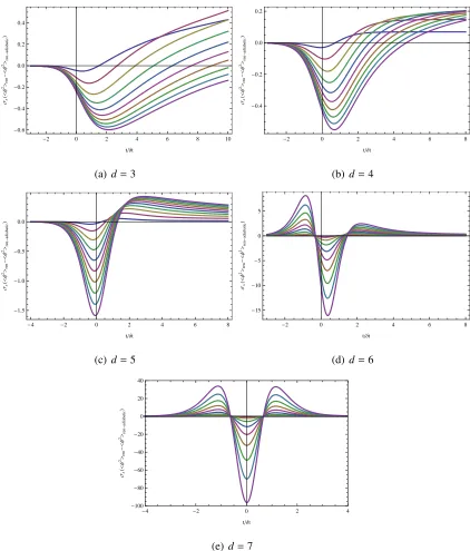
3.1 (Colour online) Renormalized expectation valueshφ2iren as a function of time

t/δt, ford = 3 and 4. In each plot, the different curves correspond to different quench rates:δt=1/1,1/2,· · · ,1/10 where the curves exhibiting higher peaks (in absolute value) correspond to smaller values ofδt. Note that the expectation value is multiplied by the numerical constant σs = 2(2

π)d−1

Ωd−2 . Further, at each

time, the expectation value for an ‘adiabatic’ quench is subtracted. . . 51 3.2 (Colour online) Renormalized expectation valueshφ2_i

ren as a function of time

t/δt, for d = 8 and 9. In each plot, the different curves correspond to dif-ferent quench rates: δt = 1/20,1/21,· · · ,1/30 where the curves exhibiting higher peaks (in absolute value) correspond to smaller values ofδt. As in the previous figure, the expectation value is multiplied by the numerical constant

σs = 2(2π)

d−1

Ωd−2 . Further, at each time, the expectation value for an ‘adiabatic’

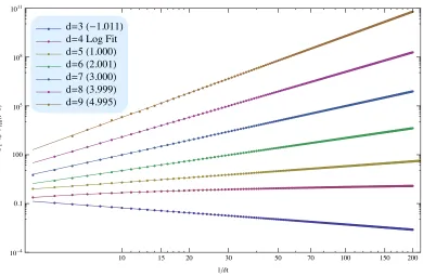
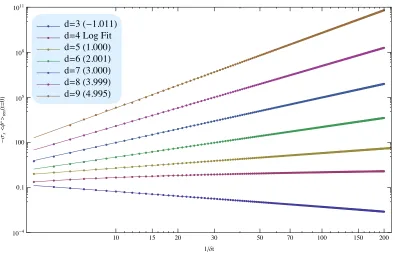
quench is subtracted. . . 53 3.3 (Colour online) Expectation value hφ2iren(t = 0) as a function of the quench

timesδt for spacetime dimensions from d = 3 to 9. Note that in the plot, the expectation values are multiplied by the numerical factor: σs = 2(2

π)d−1

Ωd−2 . The

slope of the linear fit in each case is shown in the brackets beside the labels. The results support the power law scalinghφ2iren ∼δt4−d. . . 54

(13)

time dimensions d = 6 andd = 8 — the lower curve corresponds to d = 6. As in previous plots, the expectation values are multiplied byσs = 2(2

π)d−1

Ωd−2 . We

show in a blue solid curve the best fit by a function f(δt) = δt−α₍_a_logδ_t+_b_),

where we getα=1.9995 ford =6 andα= 4.0097 ford=8. The purple curve is the best fit for a function f(δt)= aδt4−d_{. The plots clearly show that there is}

an extra logarithmic divergence in expectation values. The results support the scalinghφ2_i

ren ∝δt4−dlog(δt) for evend. . . 54

3.5 (Colour online)δtd−4hφ2_i

ren for different values of δt in odd spacetime

dimen-sions. The curves approach the analytical leading order solution (3.45), shown as the dashed red line, as δt gets smaller. In panel (a) for d = 5, running from top to bottom on the left hand side, the solid lines correspond to δt =

{1,1/2,1/5,1/10,1/20,1/50,1/100,1/500}. Similarly from bottom to top in panel (b) ford= 7, the curves correspond toδt= {1/2,1/3,· · · ,1/10}. . . 56 3.6 (Colour online) Renormalized expectation value for different values of δt in

d = 6. Panel (a) shows δt2hφ2iren. As we reduce δt from δt = 1/10 to

δt = 1/1000, the peaks in the response continue to grow. In particular, the curves correspond toδt = {1/10,1/20,1/50,1/100,1/1000}. Panel (b) shows

δt2_hφ2_i

ren/logδt. Here as δt decreases, the curves converge to the analytic

expression (red dashed line). In this case, the amplitude of the left peak in-creases monotonically asδt shrinks and the various curves correspond toδt =

{1/10,1/20,1/30,· · · ,1/100,1/1000}. . . 58 3.7 (Colour online)σshφ2irenin three-dimensional space-time. The red curves

cor-respond to the leading order analytic expression (3.53) while the blue curves are the full numerical solution. By comparing panels (a) and (b), we can see that the difference between the two solutions is roughly of order O(δt). We can observe that apart from having an extra minus sign difference, the reverse quench in panel (c) starts from zero without needing to be shifted by the factor ofm. . . 61

(14)

3.8 (Colour online) Numerical verification of the diffeomorphism Ward identity (3.56) ford = 5. Panel (a) showshEi as a function of time. Panel (b) shows the corresponding∂thEi as a function of time (dashed) and the RHS of Ward

identity (thin solid) evaluated using our previous results. In each case, the curves from top to bottom correspond to δt = 1/10,1/20,1/30,· · · ,1/100. The straight red dashed line in panel (a) showshEifor the constant mass case (m2= 1). . . 64

3.9 (Colour online) Renormalized expectation value of the energy density as a function of time for different values ofδt. From bottom to top (on the right hand side), the different curves correspond to δt = 1/10,1/20,1/30,· · · ,1/100. Hence with decreasing δt, the curves accumulate towards the top red dashed line at late times. Note that all expectation values are multiplied by the con-stantσs = 4π. The red dashed line at the bottom corresponds to the constant

mass value (withm2 = 1) while the one at top corresponds to 1/6 — see main text for explanation of this value. . . 67

3.10 (Colour online) Time derivative of the renormalized expectation value of the energy density as a function of time for different values ofδt. Different curves correspond to δt = 1/10,1/20,1/30,· · · ,1/100, with curves with smaller δt

correspond to higher peaks. Note that all expecation values are multiplied by a constantσs = 4π. The dashed lines correspond to the time derivative ofhEiren

while the thin solid lines correspond to evaluating 1₂∂tm2(t)hφ2iren. The

agree-ment between both calculations shows that the diffeomorphism Ward identity is satisfied. . . 67

3.11 (Colour online) hφ2irenδtd−4/m2 for different values of δt and different odd

spacetime dimensionsd. The solid curves correspond toδt = 1,1/2,· · · ,1/10 withδtdecreasing as they converge to the analytical leading expression (3.45), plotted with dashed red curve. This leading term hashφ2_i(d)

ren ∼(−1)

d−1 2 ∂d−4

t m2(t).

. . . 75

(15)

tion ofδtfor different even dimensions. The blue curve corresponds tod = 4, where the fit by a functionδt−α(a1−a2logδt) gives α = 0.0028, showing the

expected logarithmic growth; the purple curve corresponds tod = 6 and the same fit givesα = 2.0006; the yellow curve corresponds to d = 8 and the fit results inα=4.0019, just as expected by our power law scaling (3.2). . . 76 3.13 (Colour online) Renormalized expectation value of φ2 at timet/δt = −0.5 as

a function of δt for different odd dimensions. The blue curve corresponds to

d = 5, where the fit by a function δt−αa1 +a2 givesα = 1.006, showing the

expected scaling; the purple curve corresponds tod = 7 and the same fit gives

α = 2.991; the yellow curve corresponds to d = 9 and the fit results in α = 4.977, just as expected by our power law scaling (3.2). . . 76 3.14 (Colour online) Expectation value of φ2 as a function of time. We are in the

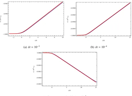
limit of t/δt 1. The solid curve corresponds to the full solution for any value ofmt. The red dashed line is the linear behaviour found in eq. (3.122) for mt 1. The orange dashed line shows the logarithmic growth found in eq. (3.124) formt1. Finally, the inset zooms in the region of smallmt. . . . 86 3.15 (Colour online) Analysis of the approximation of low energies and late times

in d = 3, with δt = 10−3 _{(where the units are set by} _m_{). Panel (a) shows}

the integrands in eqs. (3.112) and (3.119) at t = 10 but there is not visible difference between the curves. Panel (b) showshφ2_i

renas a function ofmt. The

solid blue curve corresponds to analytically integrating the expression for the instantaneous quench, eq. (3.126) ford = 3. The purple dots correspond to numerically evaluating the smooth quench expression of eq. (3.125). Again there is no visible difference between the two approaches. . . 88 3.16 (Colour online) Expectation value ofφ2as a function of time withmδt= 10−1.

The blue dots correspond to evaluating the expectation value as in section 3.2.2, while the purple dots are those coming from numerically integrating eq. (3.125). The solid line shows a fit by a function of the form f(mt) =

a+bexp(−c mt), with parametersa=0.136,b= 0.442 andc=1.349. . . 89

(16)

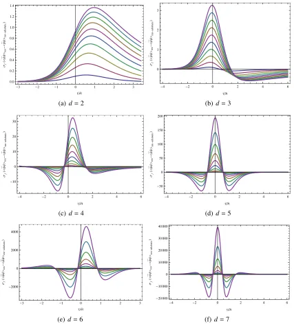
3.17 (Colour online) Renormalized expectation values of ¯ψψ as a function of time. The different curves correspond toδt = 1/1,1/2,· · · ,1/10. The curves are so that higher peaks (in absolute value) correspond to smaller δt. Note also that we are plotting the expectation value multiplied by the numerical constantσf

that depends on the spacetime dimension. Also note that we are subtracting at each time the expectation value in the adiabatic case, for which we are using

δt = 10. In even spacetime dimension d, the plots corresponds to having the renormalization scale set tok0 =1. . . 94

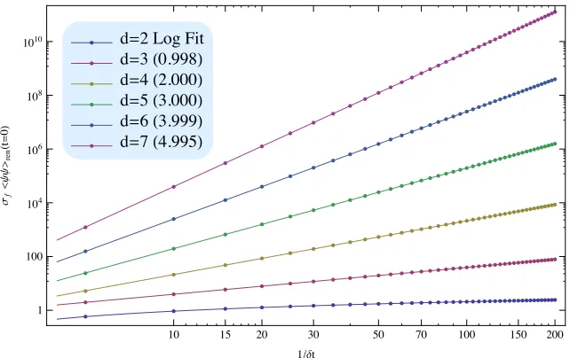
3.18 (Colour online) Expectation value hψψ¯ iren(t = 0) as a function of the quench

timesδtfor spacetime dimensions from d = 2 tod = 7. Note that in the plot, the expectation values are multiplied by a numerical factor σf depending on

the dimension. The slope of the linear fit in each case is shown in the brackets beside the labels. The results support the power law scalinghψψ¯ iren ∼δt−(d−2). . 95

3.19 (Colour online)hψψ¯ irenδtd−2 for different values ofδtand different odd

space-time dimensionsd. As the curves approach the leading order analytic solution (3.140) shown with the dashed red line,δtgets smaller, with solid (numerical) curves going fromδt = 1 toδt = 1/10. Ford = 3 we also included the curves withδt =1/50 and 1/100. . . 96

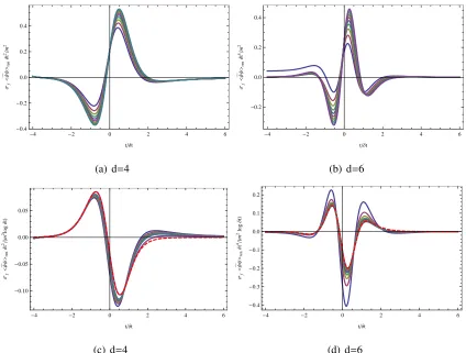
3.20 (Colour online)hψψ¯ iren for different values ofδtind = 4 and 6. In panels (a)

and (b), we only divide by the expected power-law scaling. As we reduce δt

from δt = 1/10 to δt = 1/100 for d = 4 and from δt = 1 to δt = 1/10 for

d = 6, we see that the expectation value still grows, indicating the presence of an extra logarithmic factor. If we take the latter into account and divide by it as well, we find panels (c) and (d), where we see that the curves now converge towards the analytic expression (red dashed line). . . 97

(17)

d= 5,t= 10,r =10 andδt =1/20 as a function of momentumk— all dimen-sionful quantities are given in units of the initial massm. All three integrands are nearly identical for large momenta. Further the instantaneous and smooth quench curves overlap at all scales. . . 133

4.2 (Colour online) Subtracted integrands as a function of (small) momentumk. In this case we are plotting ford =5,t=10,r= 10 (with the units set bym). The yellow line corresponds to the instantaneous quench while the blue one to the smooth. Panel (a) shows that no detectable differences appear withδt = 1/20 in the range 0≤ k ≤ 2. However, in panel (b), minor differences occur in this range whenδt=1/2. . . 134

4.3 (Colour online) Subtracted integrands as a function of momentum k. In this case we are plotting ford =5, t= 10,r= 10 andδt =1/20 (with the units set bym). The blue line corresponds to the smooth quench while the yellow one to the instantaneous quench. Panel (a) shows an intermediate regime where no significant differences between the two integrands are apparent. Visible differences appear for largerk &1/δt, in panel (b). . . 135

4.4 (Colour online) Regulated integrands as a function of momentumkfor d = 5 and small separation. The blue line corresponds to the smooth quench while the yellow one to the instantaneous. At small distances the two integrands are clearly different from each other, even at scaleskδt≤1. . . 135

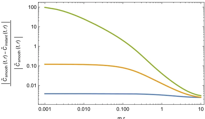
4.5 (Colour online) Difference between the late-time correlators for smooth and instantaneous quenches as a function of the separation distance r. The blue line corresponds to thed = 3 case while the yellow one belongs tod = 5 and

d= 7 is shown in green. We are usingmt =10 withmδt= 1/20. Ind = 3 and

d= 5, the difference remains small for any value ofr, while ind = 7, it seems to diverge asr→0. . . 136

(18)

4.6 (Colour online) Spatial correlator under a smooth quench att= 0 as a function of both δt and the distance separation r. In each case, we are subtracting the fixed mass correlator withm2= 1/2. The dashed lines correspond to computing the instantaneous quench correlator att =0 for the different separationsr, that is the same as computing the fixed mass correlator with m = min = 1. The

purple solid line shows the analytic leading order contribution tohφ2_i_{, given by}

eq. (4.44). . . 144

4.7 (Colour online) Spatial correlator under a smooth quench for fixedt/δt =τas a function of bothδtand the distance separationr. In each case, we are subtract-ing the fixed mass correlator withm2(t/δt=τ). The dashed lines correspond to computing the fixed mass quench correlator withm=min for the different

sep-arationsr. The purple solid line shows the analytic leading order contribution tohφ2_i_{, given by eq. (4.44). . . 145}

4.8 (Colour online) Analysis of the approximation of low energies and late times ind = 5. We show results forδt = 10−3,t = 10 andm = 1. In the first figure, we show that Φ2₍_k_{) in both eqs. (4.57) and (4.58) coincide when evaluated}

for smallk. However in the second plot, we see that the full integrand (blue) decays for largekwhile the approximate solution (red) keeps oscillating. The second plot looks fully painted because of the highly oscillatory nature of the functions. . . 149

4.9 (Colour online) Analysis of the approximation of low energies and late times ind = 7. We show results forδt = 10−3_,_t = _{10 and}_m = _{1. In the first figure,}

we show that Φ2(k) of both eqs. (4.57) and (4.58) coincide when evaluated for smallk. However in the second plot, we see that the full integrand (blue) decays for largekwhile the approximate solution (red) keeps oscillating. The second plot looks fully painted because of the highly oscillatory nature of the functions. . . 150

(19)

tion of the regulator parametera ford = 5 and mt = 10. The values of ago from 10−1to 10−4in a logarithmic scale. The solid line represents the value for the smooth quench atmt= 10 andδt= 1/20. . . 152

4.11 (Colour online) Relative error in the computation ofhφ2_i_{at late times using the}

smooth and the instantaneous quench as a funtion ofδt. Here we are regulating the instantaneous result with a = 10−3 _{and evaluating at time} _mt = _{10. The}

red dashed line is showing the fit of the first points (from δt = 1/1000 to

δt= 1/800) by a power law function of the type f(δt)=aδtα, wherea=20.03 andα= 1.404. The inset zooms in the region where the fit was made showing perfect agreement between the points and the fit. . . 154

4.12 (Colour online) The integral I1(λ) in eq. (4.75) as a function of λon a

loga-rithmic scale. The data are ford =2,3,4,5,6,7 from top to bottom. The solid lines correspond to I1(λ) ∼ λd for d = 2,3 and I1(λ) ∼ λ4 for d = 4,5,6,7.

Note that the fit ind= 4 is not as good as the others, which suggests that there are log corrections to the leading behavior ford= 4. . . 157

4.13 (Colour online) The absolute value ofI2(λ)= m−dδEas a function ofλ= mδt

on a logarithmic scale. The data are for d = 2,3 from bottom to top. The solid lines correspond to the curves I2(λ) ∼ λ2 for d = 2 and λ for d = 3.

Those curves correspond to the best fit of the numerical data in the region 10−7 < λ <10−5. . . 158

(20)

4.14 (Colour online) Schematic description of the evolution of the energy density after a quench as a function of time depending on the regularization scheme. In the first row we exemplify the counterterm subtraction that allows us to follow the evolution for any time, even during the quench itself, characterized by the time scale δt. Taking the counterterm energy density as the zero of energy density, at very early times, the starting energy density is negative for

d= 4k+3 and positive ford =4k+1, withk≥ 0 integer. In the second row we take the fixed energy density as the zero of energy density. In this case, all the quench energies are greater than this ground zero energy density. The reason is that the fixed mass energy density is the energy density for the scalar with a fixed mass and no quench, so any energy inserted during the quench will give a positive additional contribution. Note that in low dimensional spacetimes, the fixed energy density differs from the counterterm energy density but always by a finite amount proportional to a power of the mass at that instant of time, while the quench energy density usually scales also withδt, so our universal scalings,

i.e.,δE ∼ δλ2δ_td−2∆_{, will appear in any case. The same will happen in greater}

dimensions at very early and very late times. However, ford ≥ 6 during the quench, it is not sufficient to subtract the fixed energy density, as there are extra UV divergences in the quenched energy density that are proportional to time derivatives of the mass. In this case, subtracting the fixed energy density is sufficient to compute the energy density at very early or very late times but not during the middle of the quench. This is depicted in the plot in the bottom-right corner ford = 7 but is a general feature of higher dimensional spacetimes. In the same way, in the upper-right plot we cannot sketchEf ixed− Ectduring the

quench as they differ by an infinite amount. . . 166

4.15 (Colour online) Schematic plots of the evolution of the energy density in three spacetime dimensions when δt → 0. From the counterterm subtraction point of view, the work done is zero but from the fixed mass subtraction perspective, there is finite work done. . . 169

(21)

5.2 Evidence for KZ physics near a critical point in fermionic quenches. The green solid line represents the adiabatic solution at each instant of time. The blue dots correspond to the expectation value of the mass operator for a slow quench with δt = 10, in units of m. In fig. (a) we see that for early and late times the expectation value follows the adiabatic expectation for slow quenches. In fig. (b) we focus on the region near the critical point (t = 0), and in fact, we see that the expectation value differs from the adiabatic one. As a guide we plotted in dashed red lines plus and minus the Kibble-Zurek time,±τKZ =

±1/√mδt, were we should expect the two curves to start differing from each other, according to the original Kibble-Zurek argument. As we see in fig. (b), this is in fact what is happening. . . 189 5.3 Evidence for KZ physics near a critical point in pulsed scalar quenches. The

green solid line represents the adiabatic solution at each instant of time. The blue dots correspond to the expectation value of the mass operator for a slow quench withδt= 10, in units ofm. In fig. (a) we see that for early and late times the expectation value follows the adiabatic expectation for slow quenches. In fig. (b) we focus on the region near the critical point (t = 0), and in fact, we see that the expectation value differs from the adiabatic one. As a guide we plotted in dashed red lines plus and minus the Kibble-Zurek time,±τKZ =

±1/√mδt, were we should expect the two curves to start differing from each other, according to the original Kibble-Zurek argument. As we see in fig. (b), this is in fact what is happening. . . 190 5.4 Renormalizad expectation value of fermionic mass operator as a function of

t/tKZ for d = 5. The different curves correspond to δt = 10i, with i =

0.5(blue),1(yellow),1.5(green),2(orange), in units ofm. Note that we are mul-tiplying the expectation value by δt5−21, that is the expected KZ scaling. In

dashed red, we plotted the expectation value in the adiabatic case. In fig. (a) we plotted for large periods of time, while in fig. (b) we zoomed in the area where we expect KZ scaling to appear (−1< t/tKZ <1). . . 191

(22)

5.5 The transition from the fast quench to the slow quench att = 0 for fermionic quenches. The fast quench exhibits the usual fast quench universal scaling. The leading analytical contribution were found in [7, 8] and they are plotted in solid orange. In solid purple we have the best fit lines for the slow regime, with powers of δt supporting the KZ scaling hψψ¯ iren ∼ δt−

d−1

2 . At t = 0, the two

regimes are divided by the scalemδt = 1, which is plotted in dashed red for orientation purposes only. . . 193

5.6 The transition from the fast quench to the slow quench att = 0 for the scalar quench. The fast quench exhibits the usual fast quench universal scaling. The solid orange curve is the leading order contribution for fast quenches, that as we are in even dimensions, it has an extra logarithmic contribution. The solid purple curves show the KZ scaling,hφ2_i

ren ∼ δt−

d−2

2 , that is enhanced ind = 6

by a logarithmic contribution, that is not present ind = 4. In each figure, the inset shows the same expectation value but notin logarithmic scale, near the region where the apparent divergences appear. As it can be easily appreciated, the profiles are smooth and the apparent divergent behaviour is just an artifact of the logarithmic scale when the expectation value changes sign. . . 194

5.7 Expectation value of the fermionic mass operator at fixedτ= −1/5, as a func-tion ofδt. We set the mass to m = 1. The solid organge line is the analytic leading contribution to the expectation value for fast quenches; the solid pur-ple line agrees with the KZ scaling,hψψ¯ iren ∼ δt−

d−1

2 ; and the solid green line

shows the adiabatic value for a fixed-mass operator with the corresponding mass atτ = −1/5. To guide the different regions we also plotted dashed red lines atδt= 1 andδt=1/τ2, that should correspond to the transition scales. . . 200

(23)

function ofδt ford = 5. We set the mass tom = 1. The solid organge line is the analytic leading contribution to the expectation value for fast quenches; the solid purple line agrees with the KZ scaling,hφ2_i

ren ∼ δt−

d−2

2 (the fit by a

func-tiony=ax−αgivesa= 0.1867 andα= 1.515) ; and the solid green line shows the adiabatic value for a fixed-mass operator with the corresponding mass at

τ = −1/16. To guide the different regions we also plotted dashed red lines at

δt =1 andδt =1/τ2_{, that should correspond to the transition scales. Note that}

as there is a change of sign in the expectation value, noticeable in the plot by an apparent divergence aroundδt∼ 10−1_{, we decided to plot the absolute value}

of the renormalized expectation value. To avoid misinterpretations, we also in-cluded an inset without the logarithmic scale to show that the expectation value is smooth as a function ofδt. . . 201

5.9 Renormalizad expectation value ofφ2_{as a function of}_t/_t

KZ ford =5. The

dif-ferent curves correspond toδt=10i, withi=0.5(blue),1(yellow),1.5(green),2(orange), in units ofm. Note that we are multiplying the expectation value byδt5−22, that

is the expected KZ scaling. In dashed red, we plotted the expectation value in the adiabatic case. In dashed green, we present the leading order solution in the large κ expansion. In fig. (a) we plotted for large periods of time, while in fig. (b) we zoomed in the area where we expect KZ scaling to ap-pear (−1< t/tKZ <1). . . 204

5.10 Expectation value of the scalar pulsed mass operator at fixed τ= −1/16, as a function of large δt for d = 5. We set the mass to m = 1. The solid green line shows the leading order solution in the κ expansion, δt−3/2F(−√δt/16). To guide the different regions we also plotted dashed red lines at δt = 1 and

δt= 1/τ2, that should correspond to the transition scales. . . 205

(24)

5.11 Expectation value of the scalar mass operator at fixedτ= 12, as a function of

δt. We set the mass tom = 1 and concentrate on large quench rates. The solid purple line is the best fit for the points in the Kibble-Zurek regime and obeys the equation y = aδt−α_{, with} _a = ₀._{0199 and} α = ₂._{993, which supports the}

conclusion that in these exponential protocols the relevant scale ismKZ instead

oftKZ. The green line corresponds to the adiabatic value atτ= 12. . . 207

5.12 The value of δt at which there is a transition between the KZ scaling and the adiabatic behaviour as a function of the fixed timeτ. The curve corresponds to an exponential fit of the numerical points (y=aexp(−τ), witha=0.314). This is in agreement with expectations given by eq. (5.70), though it is not exact as we are taking δtKZ as the intersection between the KZ fit —purple line in fig.

(5.11)— and the adiabatic value). . . 208

(25)

5.1 Description of free field theory quenches. . . 180

(26)

List of Abbreviations, Symbols and

Nomenclature

(A)dSd : d-dimensional (Anti)-de Sitter spacetime

Sd _: _d_{-dimensional Sphere}

d : spacetimedimensions

CFT : Conformal Field Theory QFT : Quantum Field Theory UV : Ultraviolet

IR : Infrared

RHIC : Relativistic Heavy Ion Collider LHC : Large Hadron Collider

QCD : Quantum Chromo-Dynamics QGP : Quark Gluon Plasma

EE : Entanglement Entropy

h · iren : Renormalized Expectation Value

~ : Planck Constant kB : Boltzmann Constant

KZ : Kibble-Zurek

TCP : Trans-Critical Protocol CCP : Cis-Critical Protocol ECP : End-Critical Protocol

(27)

In this Thesis, I presented results related to universal behaviour of quantum field theories after a quantum quench that came up as part of a collaboration with Prof. Sumit R. Das at University of Kentucky and Prof. Robert C. Myers at Perimeter Institute for Theoretical Physics. The idea behind these studies was to generalize previous results obtained in the context of holography to more general grounds. In fact, we argue that the scaling found for smooth fast quenches is indeed universal and valid beyond holographic theories.

The scaling found implies that for operators with scaling dimension ∆ > d/2, the expec-tation value for the quenched operator as well as the expecexpec-tation value for the energy density diverge in the limit in which the quench duration goes to zero. This highlights the importance of the quench duration in the study of these far-from-equilibrium protocols and makes mani-fest that some of the ideas involving instantaneous quenches should be revised. In this sense, this Thesis should be read as a bridge between high-energy and condensed-matter studies on quantum quenches. It is an invitation for the high-energy community to go beyond holographic studies but it is also an invitation to the condensed-matter community to go beyond the abrupt limit. We hope to have provided at least the initial steps in these directions and that future results will reinforce this idea of collaboration between different areas in theoretical physics and even reach experimentalists.

This Thesis is a compilation of the articles we wrote as part of this collaboration. There are four different articles, three of which have already been published in international journals and one that is still to be published. But during my time as a graduate student at Western University and the Perimeter Institute, I had the opportunity to work on other interesting projects that I would like to briefly mention in this Preface.

The first one was entitled “Holographic R´enyi entropies at finite coupling” and was written

(28)

in collaboration with Prof. Robert C. Myers. The work was published in the Journal for High Energy Physics and can be found in JHEP 1308 (2013) 063, http://arxiv.org/abs/arXiv:1305.7191. We computed Rényi entropies (a one-parameter family generalization of the well-known en-tanglement entropy) for a spherical entangling surface in four-dimensionalN =4 super-Yang-Mills at strong coupling using the AdS/CFT correspondence. In [1102.0440], it was shown that the computation of entanglement entropy for a sphere in the ground state of an holo-graphic CFT can be mapped to thermal entropy in a topological black hole whose horizon exhibits an hyperbolic geometry. The temperature of the black hole is associated with the rank of the Rényi entropies. In this work we computed the leading order corrections to the Rényi entropies in inverse powers of the ’t Hooft coupling and the number of colours. In the gravity side, this corresponds to include the leadingα0 corrections to the low energy effective action. Even though the calculation of entanglement entropies at finite coupling can be in general a very difficult task, we used the fact that we know how to compute thermal entropies in higher derivative theories of gravity to complete the calculation. As expected, we found that when the rank of the Rényi entropy qgoes to 1, then there are no corrections due to the known result that the universal part of the entanglement entropy is proportional to the central charge of the theory. We also found an interesting relation between theq→0 limit and the free energy of the system, finding the same correction in that limit as in the free energy case. We also computed the leading corrections to the scaling dimensions of the twist operators.

A second project was started in collaboration with my supervisor Prof. Alex Buchel. This one was entitled “Cascading gauge theory ondS4and String Theory landscape” and was

pub-lished in Nucl.Phys. B883 (2014) 107-148, http://arxiv.org/abs/1310.1372. One of the ways to construct de Sitter vacua in String Theory is to place anti-D3 branes at the tip of the conifold in Klebanov-Strassler geometry. A local geometry of such vacua exhibit gravitational solu-tions with a D3 charge measured at the tip opposite to the asymptotic charge. We numerically constructed the full solutions for anti-D3 branes that are smeared at the tip. These are gravity duals of cascading gauge theories on dS4. We analysed chiral symmetry breaking in these

geometries, finding that the D3 charge is zero in the phase that spontaneously breaks the chiral symmetry. In the unbroken phase, the charge is always positive. This presents a difficulty in trying to uplift the AdS solution to a dS one, where the D3 charge should be negative.

(29)

the Einstein equation from extremizing the vacuum entanglement entropy for small spheres [1505.04753]. Trying to check one of Jacobson’s assumptions we started a project with Prof. Robert C. Myers and Prof. Horacio Casini from Instituto Balseiro in Bariloche, Argentina. The results can be found in a paper called “Comments on Jacobson’s ’Entanglement equilib-rium and the Einstein equation’ ”, that at this moment has only been submitted to the arXiv, http://arxiv.org/abs/1601.00528. We analyze the holographic problem, where a scalar field in AdS is dual to a relevant operator of dimension ∆. By choosing appropriate boundary con-ditions for the scalar field we can tune the field theory to be non-conformal by turning on a coupling and an expectation value for the operator. We can then compute the variation in entanglement entropy. It turns out that the answer depends on the scaling dimension of the operator: ford/2 < ∆ < d, the leading contribution to the entanglement entropy is given by a precise combination of the energy density and the trace of the stress-tensor, and even though is not precisely the one postulated in Jacobson’s original proposal, it is still sufficient to derive the gravity equations from there; for ∆ = d/2, there is an extra logarithmic contribution to the entanglement entropy, whose final contribution to the Einstein equation should be carefully analysed; and for d/2−1 < ∆ < d/2, the leading contribution stops being the one given by the stress tensor. On the contrary there is a contribution given by the expectation value of the operator squared, that will be the first contribution given that∆is in this regime and the size of the ball is small enough. This poses a challenge to Jacobson’s derivation but we also discuss in the paper different ways of circumventing the problem.

The interested reader might find it useful to also take a look at these other publications. I hope the idea of excluding these papers from the main body of the Thesis would be the correct one and would help to present a more coherent and concise story. But so far, the reader found a lot about my other interests but not much about quantum quenches, so it is already time to go into the main text. I hope you will enjoy it as much as I enjoyed researching on all these subjects.

D.A.G. February 7, 2016

(30)

Chapter 1 Introduction

This Thesis is mainly devoted to the study of smooth quantum quenches and the appearance of universal scaling properties in different regimes depending on the quench durationδt. The idea behind a quantum quench is to follow the evolution of an isolated quantum system when one of the couplings in the theory is modified. In a series of papers [1–4], we found several uni-versal properties for expectation values undergoing quantum quenches. The quench protocol is one of the few insights we have so far into far-from-equilibrium physics and thus, consti-tutes an interesting problem to study by itself. However, as a high energy physicist, there are extra motivations to think about this problem that are related to string theory and the so-called holographic or AdS/CFT correspondence [5].

It is the aim of this Introduction to give a brief overview on how the quantum quench prob-lem appears in string theory. We will show how through the AdS/CFT correspondence, high energy theorists can get in contact to actual experimental physics such as the quark-gluon plasma experiments. Then, we will review some specific results on holographic quantum quenches that serve as our specific motivation to study smooth quenches in a broader set of quantum field theories beyond holography. As with many other important concepts in high energy physics, quantum quenches were first discussed in the condensed matter community. So we will then review how the concept arises in the context of ultra cold atoms experiments and describe the instantaneous quench protocol that is widely used in the condensed matter literature.

We will then finish this Introduction by giving an outline of the present Thesis, that is

(31)

intended to provide a bridge between the high energy and the condensed matter approach to quantum quenches. Eventually, the universal scaling relations described in this Thesis might become part of the list of results that were first discovered in the context of string theory but have finally become available in experimental setups.

1.1 String theory, holography and quantum quenches

At present, our best understood knowledge of nature at its fundamental level relies on two different frameworks: the one prescribed by General Relativity, that describes gravity; and Quantum Mechanics, responsible for the rest of the fundamental interactions. There has been many attempts in the last century to formulate a unifying theory of quantum gravity but so far none of them has completely succeeded.

One of the most promising attempts is string theory [6, 7]. The idea behind it is to as-sume that the fundamental objects of the theory, instead of being point-like particles, are 1-dimensional strings. The introduction of these extended objects is supposed to cure the usual divergences that appear in QFT. Moreover, by quantizing the string action we obtain, in the low energy spectrum, a massless spin-2 particle that would play the role of the graviton. Both facts seemed very promising for a candidate to a “quantum theory of everything”. Though the original formulation was through a bosonic string, it was possible to formulate a stable theory with fermions by introducing supersymmetry. Apart from this, superstring theories require spacetime to be ten-dimensional. So, if we are willing to describe our universe with strings, we should understand what happens with the extra 6 dimensions and why we do not observe them. The idea of compactifying these extra dimensions gave rise to the appearance of lots of beautiful mathematical structures in String Theory but also posed a big challenge to string phe-nomenologists as the number of vacua that could describe our universe became exponentially large [8].

(32)

1.1. String theory,holography and quantum quenches 3

it is often called “holographic duality”. To be more precise, in his original paper Maldacena proposed the duality between type IIB string theory onAdS5×S5andN =4 super Yang-Mills

in four spacetime dimensions. The need of anAdS geometry is deeply related to the fact that the field theory needs to be conformal so it is also well-known as AdS/CFT correspondence or gauge/gravity duality.

Soon after the proposal, Gubser, Klebanov and Polyakov [10] and, independently, Wit-ten [11] established precisely the meaning of the duality by proposing the equivalence of the partition functions by what is known now as the GKPW ansatz. It was proposed that in order to compute expectation values in the CFT side, one should evaluate the partition function in the string theory side, with a scalarφfunctioning as the source for the operatorOin the boundary. Formally,

lim

φ→φ0

Zs[φ]= lim

φ→φ0

e−Sstring[φ] _{≡ h}_e− R

Bφ0Oˆi

CFT , (1.1)

whereZs is the partition function for the string theory, that is given as the exponential of the

string actionSstring.

The correspondence opens double-way opportunities: it becomes possible to make compu-tations in the field theory side to learn about string theory and/or to perform analysis in string theory to learn about conformal field theories. These possibilities are somehow enhanced by the fact that this is also a weak/strong duality. In particular, according to the holographic dic-tionary ls ∝ 1/

√

λ, where ls is the string length in units of the AdS radius and λ is the ’t

Hooft coupling for the field theory. Adding the extra limit of the gauge rank N in the gauge theory going to infinity, then the correspondence relates a strongly-coupled conformal field theory at large-N, with classical Einstein gravity theory in extra dimensions. Given that fact, the AdS/CFT correspondence is now one of the only tools to make analytic predictions in strongly-coupled theories, where the usual perturbation theory approaches are not useful.

(33)

relativistic speeds before they collide. Rapidly after the collision, the system achieves thermal equilibrium and forms what is known as the quark-gluon plasma. After some time, it freezes down and goes to a hadronization phase forming the different particles that are later detected in the detectors of the experiments. An important feature of this plasma is that it turns out to be strongly-coupled [12, 13].

This served as an opportunity to use the holographic duality to get insight into what was going on in real experiments. Of course, the QCD plasma does not behave exactly in the same way as theN = 4, large-N plasma, but at finite temperature and strong coupling they should have similar properties, at least qualitatively [14].

One of the most interesting properties that was predicted by holography is the ratio between the shear viscosity and the entropy density of the plasma. This is the so-calledη/sratio. It was found that this ratio in holography was universal and gaveη/s= ~/(4πkB) [15–17]. This is an

extremely small number, given that the same calculation at weak coupling diverges at leading order in the coupling [18], so it was proposed [18] as a lower bound on the value of η/s in existing fluids. It turned out later that it was possible to violate that bound in theories with gravity duals with higher curvature corrections [19]. However, it was indeed measured thatη/s

is small and near to the value predicted by holography in the quark-gluon plasma experiments, probably being this the first important prediction of string theory in experimental physics [12].

The other salient aspect of the quark-gluon plasma experiment that holography could ex-plain is the rapid thermalization rates. In fact, in holography, a thermal state in the boundary is dual to a black hole geometry in the bulk. So the process of thermalization is dual to black hole formation in AdS. Both analytic arguments [20] and numerical simulations in gravity [21] suggested that the thermalization rates in the quark-gluon plasma should be extremely short. These works made it manifest that it was possible to study very rapid changes under hologra-phy. In particular, these models simulated thermalquenches, in which the temperature of the system changed rapidly, but also motivated the study of more general holographic quantum

(34)

1.2. Holographic dual of a quantum quench 5

1.2 Holographic dual of a quantum quench

The idea is to find a gravitational dual to a system that can be described with the following action

S =SCFT +

Z

ddxλ(t)O_∆(~x), (1.2)

which is a deformation of the CFT indspacetime dimensions.λ(t) is the coupling that we will be quenching and we will be interested in following the evolution of the expectation value of the relevant operatorO_∆, with conformal dimension∆.

According to the AdS/CFT dictionary [5], the dual gravitational action ind+1 dimensions yields

Sd+1 =

1 16πGN

Z

dd+1x√−g R−2Λ− (∂φ)

2

2 −

m2φ2

2 −V(φ)

!

, (1.3)

where apart from the metricgand a negative cosmological constantΛ, we introduced a massive scalar field φthat will be dual to the CFT operator O_∆. We also added a potential V(φ), that only contains terms cubic in φ or higher order. The mass of the scalar field is related to the conformal dimension of the boundary operator through the usual formulam2 = ∆(∆−d), where the mass is given in units of the AdS radius [5].

This is the general setup for the holographic problem. In this Thesis, we will be generally interested in homogeneous and isotropic solutions (in the boundary spatial directions), so we can assume some symmetry in the ansatz for the metric. In particular, we will only allow the metric functions to depend on time and on the holographic coordinate. In Poincar´e coordinates where the AdS metric (with unit radius) is given by

ds2_AdS

d+1 =

dz2−dt2+d~x2

z2 , (1.4)

the bulk metric becomes

(35)

whereA(t,z) andΣ(t,z) are the functions that will determine the metric solution.

The next step is to compute the equations of motion for this gravity-scalar system. This problem was studied, for instance, in [22–24]. In general evolving the gravitational equations for the full spacetime as a function of time can be a challenging task, that usually needs the use of heavy computational techniques. For d = 4 that analysis was done in [23]. In addi-tion, in [24], it was found that it was possible to reproduce the leading order scaling by doing completely analytical computations.

Near the boundary, the scalar field will have an asymptotic expansion of the form

φ(t,z)∼zd−∆(p0(t)+O(z2))+zd(p2∆−d(t)+O(z2)), (1.6)

where p0(t) is usually called the non-normalizable coefficient and will be proportional to the

couplingλin the field theory side and the normalizable coefficientp2∆−d(t) will be proportional

to the expectation value of the operatorO_∆. Then the holographic problem dual to a quantum quench consists of specifying a profile for p0(t) that varies as a function of t/δt, with δt the

quench duration, and then solving the gravitational equations of motion to find the response

p2∆−d(t), that will be dual to the evolution for the expectation value of the quenched operator.

Once the gravitational problem is solved, we need to go back to the field theory side to analyze the different observables of interest. This is done by what is called the method of holo-graphic renormalization [25–27], where counterterms are added in the form of boundary terms in the action in order to cancel divergences in the gravitational solution. This was performed numerically in detail in [23] and as a result they found that for fast quenches,

hO_∆iren ∼δλ/δt2d

−∆_,

(1.7)

(36)

1.3. Quantum quenches in condensed matter 7

AdS vacuum. For protocols of the form p0(t)=δp(t/δt)κ, it turns out that

p2∆−d(t)=

2d−2∆Γ₍κ+₁₎Γ₍d+2−2∆

2 )

Γ(d+1+κ−2∆)Γ(2∆−₂d+2)δp/δt

2∆−d

(t/δt)d−2∆+κ, (1.8) which again depicts the same universal scaling relation for fast quenches in the context of holography.

Of course, this result was one of the main motivations to study fast smooth quenches in other non-holographic settings. The fact the this scaling was universal in holography served as an indication that it might have much broader implications. However, at this point, we must mention that it is not at all trivial to generalize holographic results to general CFTs. In particular, when we describe holographic theories in this context we are assuming, at least, that the field theories are infinitely strongly coupled and that they have an infinite number of degrees of freedom. That is what allows us to use the classical Einstein action for the present computations. Moreover, most of the concrete known examples of holographic theories are also supersymmetric theories. So it might well have been the case that the scaling found was only universal for holographic theories but not valid in a more general context. A large part of this Thesis is devoted to prove that those results are valid beyond holography.

For now, we should note an appealing property of this scaling, that will also need further study. Assuming the scaling dimension of the operator is greater thand/2, then the expectation value diverges asδtgoes to zero. This might just have been an extra interesting fact but nothing more than that. However, it turns out to be very important since that limit corresponds to the instantaneous quench where the change in the coupling occurs abruptly. Those are the kind of protocols that have been broadly studied in the condensed matter literature. In the next section we briefly discuss the problem of the instantaneous quench.

1.3 Quantum quenches in condensed matter

(37)

theoreti-cal exercise, since experimentalists were far from being able to simulate such situations in the laboratories. For long, creating extended quantum systems that maintain its quantum properties for a period long enough to test these theoretical expectations was nothing more than a dream. The main problem was that interactions of the quantum system with the (classical) environment made decoherence and dissipation to happen too soon making it impossible to follow the quan-tum evolution of the system. However, this changed in the last decade, where experimentalists working with ultra cold atom systems managed to create quantum systems for longer periods of time [29]. In this type of experiments, optical lattices are being created with lasers to trap atoms in a superfluid. By quickly changing the depth of this harmonic optical potentials the description of the system can change very fast from a hydrodynamics description to a lattice one, where the atoms are trapped when the potential is deep enough.

This also revived the theoretical interest in far-from-equilibrium physics following the sem-inal paper by Cardy and Calabrese [30] where the termquenchwas coined. The quench process can then be described as follows [30–32]: the system starts att = 0 in a prepared pure state,

|ψ₀i, that is generally the ground state for some initial Hamiltonian that they call H0; then,

abruptly, the system changes and is now described by a new HamiltonianH, that can be simply

H0 plus some external perturbation; now, the state evolves unitarily for t > 0 with this new

Hamiltonian. The state that was previously asimplestate in terms of the old Hamiltonian, now becomes a very non-equilibrium state in the new one.

Note that in this description the Hamiltonian changes instantaneously att =0, so basically under this framework it is only possible to study the late time and large distances behaviour of the system. Obviously, one can ask questions such as how does the system evolves, whether it thermalizes or not and, in the case it does, to what kind of thermal state.

Defined in this way, the quench problem is basically the problem of finding the decomposi-tion of one state, that was previously the ground state for some Hamiltonian, into eigenstates of the new Hamiltonian. The simplest example to show how this works is just a simple harmonic oscillator whose frequency is quenched from someω0toω[32]. In this case we start att = 0

with the ground state|Ψ₀ifor the Hamiltonian

H0= 1/2π2+1/2ω20φ

(38)

1.4. Thesis overview 9

and we want to evolve it in time with the new Hamiltonian,

H= 1/2π2+1/2ω2φ2. (1.10)

The solution at an arbitraryt>0 is then simply given by

|Ψ(t)i=e−iHt|Ψ₀i=X

n

C(t,t0), for instance, results in

C(t,t0)= (ω−ω0)

2

4ω2ω 0

cosω(t−t0)+ ω

2₋ω2 0

4ω2ω 0

cosω(t+t0)+ e

−iω|t−t0_|

2ω . (1.12) The free scalar field theory can be thought as a collection of momentum modes, each one behaving as a simple harmonic oscillator. So, assuming a relativistic dispersion relationω2 =

k2+m2, the correlator for a free field theory under a mass quench can be simply obtained by “summing” all the contributions from the individual modes. That is,

C(t,t0,r)=hΨ₀|T(φ(t,~r)φ(t0,0))|Ψ₀i=

Z ddk

(2π)de i~k·~r

C(t,t0). (1.13) In Chapter 4 we will compare in detail this correlator with the one obtained by doing a smooth quench. Of course more complex problems related to abrupt quenches can be and has been studied, see [33] for progress reviews. But for this Introduction we just wanted to give a flavour of the kind of computations that were done using the abrupt quench approximation and that will be of relevance in the following Chapters of this work.

1.4 Thesis overview

(39)

a short Letter [1]. Basically, we prove that the same scaling that appears for fast quenches in holography, see eq. (1.7), is present in free field theories where we quench the mass of the scalar/fermionic field. Moreover, we give an argument based on Conformal Perturbation Theory to claim that the expectation value for any quenched operator should scale in a similar fashion in any CFT. This means that if we have an operator O_∆ of dimension ∆, we should expect that after a quench characterized by a time scaleδt, its renormalized expectation value should scale as

hO_∆iren ∼δλ/δt2∆−d, (1.14)

whereδλis the amplitude of the quench.

Chapter 3 first appeared as an article in the Journal of High Energy Physics [2] and presents a detailed derivation of the general result in Chapter 2. We show how to compute the renor-malized expectation values in free field theories. In particular, we show that is possible to renormalize the expectation values by subtracting suitable counterterms that are obtained by doing an adiabatic expansion. We uncover an interesting structure of divergences that apart from having the expected instantaneous divergences involve time-derivatives of the coupling. We show in detail that expectation values obey the claimed universal scaling both numerically and analytically. Further more, the scaling is enhanced in even spacetime dimensions by a logarithmic factor that is also carefully studied.

In that rather long Chapter, we also analyze related interesting properties such as the scaling of the renormalized energy density, the scaling (and the construction) of higher spin currents, the special cases of low spacetime dimensions and late time behaviour after the quench. We also provide a more general argument and conditions under which a non-CFT should also obey universal scaling for fast smooth quenches.

(40)

1.4. Thesis overview 11

feature of our quenches in QFT is that even though they are fast compared to the amplitude of the quench, they are still slow compared to the cutoffscale, that we take to infinity. So the limit of δt → 0 implies reaching that scale. To avoid that problem, in that Chapter we also analyze spatial correlators after the quench. The advantage of computing these objects is that they are UV-finite and the spatial separation r gives an additional freedom to play with. We find that when the quench duration is larger thanr, then the same universal scaling appears for the spatial correlator. However, asδt → r, the correlator saturates to an instantaneous value. We also compared the smooth correlator to the abrupt one, finding that they usually coincide at late times and large separations but as the separation goes to zero, depending on the spacetime dimension, both correlators can beinfinitelydifferent. This is closely related to the fact that the instantaneous expectation value is UV divergent for large spacetime dimensions.

(41)

[1] S. R. Das, D. A. Galante and R. C. Myers, “Universal scaling in fast quantum quenches in conformal field theories,” Phys. Rev. Lett.112, 171601 (2014) [arXiv:1401.0560 [hep-th]];

[2] S. R. Das, D. A. Galante and R. C. Myers, “Universality in fast quantum quenches,” JHEP 1502, 167 (2015) [arXiv:1411.7710 [hep-th]].

[3] S. R. Das, D. A. Galante and R. C. Myers, “Smooth and fast versus instantaneous quenches in quantum field theory,” JHEP1508, 073 (2015) [arXiv:1505.05224 [hep-th]]. [4] S. R. Das, D. A. Galante and R. C. Myers, “Quantum Quench in Free Field Theory:

Universal Scaling at Any Rate,”to appear .

[5] O. Aharony, S. S. Gubser, J. M. Maldacena, H. Ooguri and Y. Oz, “Large N field theories, string theory and gravity,” Phys. Rept. 323, 183 (2000) doi:10.1016/ S0370-1573(99)00083-6 [hep-th/9905111].

[6] J. Polchinski,String Theory, (Cambdridge University Press, New York , 1998), 1st Edi-tion, Vol. I y II.

[7] M. Green, J. Schwarz, E. Witten,Superstring Theory, (Cambridge University Press, New York, 1987), 1st Edition.

[8] See, for instance,

P. Candelas, G. T. Horowitz, A. Strominger and E. Witten, “Vacuum Configurations for Superstrings,” Nucl. Phys. B258, 46 (1985). doi:10.1016/0550-3213(85)90602-9;

(42)

BIBLIOGRAPHY 13

R. Bousso and J. Polchinski, “Quantization of four form fluxes and dynamical neu-tralization of the cosmological constant,” JHEP 0006, 006 (2000) doi:10.1088/ 1126-6708/2000/06/006 [hep-th/0004134];

L. Susskind, “The Anthropic landscape of string theory,” In *Carr, Bernard (ed.): Uni-verse or multiUni-verse?* 247-266 [hep-th/0302219].

[9] J. M. Maldacena, “The Large N limit of superconformal field theories and supergrav-ity,” Int. J. Theor. Phys. 38, 1113 (1999) [Adv. Theor. Math. Phys. 2, 231 (1998)] doi:10.1023/A:1026654312961 [hep-th/9711200].

[10] S. S. Gubser, I. R. Klebanov and A. M. Polyakov, “Gauge theory correlators from noncrit-ical string theory,” Phys. Lett. B428, 105 (1998) doi:10.1016/S0370-2693(98)00377-3 [hep-th/9802109].

[11] E. Witten, “Anti-de Sitter space and holography,” Adv. Theor. Math. Phys.2, 253 (1998) [hep-th/9802150].

[12] J. Casalderrey-Solana, H. Liu, D. Mateos, K. Rajagopal and U. A. Wiedemann, “Gauge/String Duality, Hot QCD and Heavy Ion Collisions,” arXiv:1101.0618 [hep-th].

[13] E. Shuryak, “Physics of Strongly coupled Quark-Gluon Plasma,” Prog. Part. Nucl. Phys. 62, 48 (2009) doi:10.1016/j.ppnp.2008.09.001 [arXiv:0807.3033 [hep-ph]].

[14] M. Panero, “Thermodynamics of the QCD plasma and the large-N limit,” Phys. Rev. Lett. 103, 232001 (2009) doi:10.1103/PhysRevLett.103.232001 [arXiv:0907.3719 [hep-lat]].

[15] S. R. Das, G. W. Gibbons and S. D. Mathur, “Universality of low-energy absorption cross-sections for black holes,” Phys. Rev. Lett. 78, 417 (1997) doi:10.1103/PhysRevLett.78.417 [hep-th/9609052].

(43)

[17] A. Buchel and J. T. Liu, “Universality of the shear viscosity in supergravity,” Phys. Rev. Lett.93, 090602 (2004) doi:10.1103/PhysRevLett.93.090602 [hep-th/0311175].

[18] P. Kovtun, D. T. Son and A. O. Starinets, “Viscosity in strongly interacting quan-tum field theories from black hole physics,” Phys. Rev. Lett. 94, 111601 (2005) doi:10.1103/PhysRevLett.94.111601 [hep-th/0405231].

[19] A. Buchel, R. C. Myers and A. Sinha, “Beyond eta/s= 1/4 pi,” JHEP0903, 084 (2009) doi:10.1088/1126-6708/2009/03/084 [arXiv:0812.2521 [hep-th]].

[20] S. Bhattacharyya and S. Minwalla, “Weak Field Black Hole Formation in Asymptot-ically AdS Spacetimes,” JHEP 0909, 034 (2009) doi:10.1088/1126-6708/2009/09/034 [arXiv:0904.0464 [hep-th]].

[21] See, for instance, P. M. Chesler and L. G. Yaffe, “Horizon formation and far-from-equilibrium isotropization in supersymmetric Yang-Mills plasma,” Phys. Rev. Lett.102, 211601 (2009) doi:10.1103/PhysRevLett.102.211601 [arXiv:0812.2053 [hep-th]]. V. Balasubramanianet al., “Thermalization of Strongly Coupled Field Theories,” Phys. Rev. Lett. 106, 191601 (2011) doi:10.1103/PhysRevLett.106.191601 [arXiv:1012.4753 [hep-th]].

V. Balasubramanian et al., “Holographic Thermalization,” Phys. Rev. D 84, 026010 (2011) doi:10.1103/PhysRevD.84.026010 [arXiv:1103.2683 [hep-th]].

[22] A. Buchel, L. Lehner and R. C. Myers, “Thermal quenches in N=2* plasmas,” JHEP 1208, 049 (2012) doi:10.1007/JHEP08(2012)049 [arXiv:1206.6785 [hep-th]].

[23] A. Buchel, L. Lehner, R. C. Myers and A. van Niekerk, “Quantum quenches of holographic plasmas,” JHEP 1305, 067 (2013) doi:10.1007/JHEP05(2013)067 [arXiv:1302.2924 [hep-th]].

(44)

BIBLIOGRAPHY 15

[25] V. Balasubramanian and P. Kraus, “A Stress tensor for Anti-de Sitter gravity,” Commun. Math. Phys.208, 413 (1999) doi:10.1007/s002200050764 [hep-th/9902121].

[26] R. Emparan, C. V. Johnson and R. C. Myers, “Surface terms as counterterms in the AdS /CFT correspondence,” Phys. Rev. D60(1999) 104001 [hep-th/9903238].

[27] K. Skenderis, “Lecture notes on holographic renormalization,” Class. Quant. Grav. 19, 5849 (2002) doi:10.1088/0264-9381/19/22/306 [hep-th/0209067].

[28] E. Barouch and B. McCoy, Phys. Rev. A2, 1075 (1970);3, 786 (1971);3, 2137 (1971). [29] M. Greiner et al., “ Quantum phase transition from a superfluid to a Mott insulator in a

gas of ultracold atoms,” Nature (London)415, 39 (2002).

[30] P. Calabrese and J. L. Cardy, “Time-dependence of correlation func-tions following a quantum quench,” Phys. Rev. Lett. 96, 136801 (2006) doi:10.1103/PhysRevLett.96.136801 [cond-mat/0601225].

[31] P. Calabrese and J. Cardy, “Quantum Quenches in Extended Systems,” J. Stat. Mech. 0706, P06008 (2007) doi:10.1088/1742-5468/2007/06/P06008 [arXiv:0704.1880 [cond-mat.stat-mech]].

[32] S. Sotiriadis and J. Cardy, “Quantum quench in interacting field theory: A Self-consistent approximation,” Phys. Rev. B 81, 134305 (2010) doi:10.1103/PhysRevB.81.134305 [arXiv:1002.0167 [quant-ph]].

[33] S. Mondal, D. Sen and K. Sengupta, “Non-equilibrium dynamics of quantum sys-tems: order parameter evolution, defect generation, and qubit transfer,” Quantum

Quenching, Anealing and Computation, Lecture notes in Physics, 802, 21 (2010)

[arXiv:0908.2922[cond-mat.stat-mech]];