Three-Dimensional Laser Radar Range Imagery of Complex Target
with Rough Surfaces
Hanlu Zhang1, * and Biao Wang2, 3
Abstract—A backscattering model of the average signal power function (SPF) for laser radar 3D range imagery obtained using detector arrays for a complex target with rough surfaces is presented. The model relates the average power at the receiver to the laser pulse, target shape, optical scattering properties of the surface materials, angle of incidence, and other factors. The optical scattering properties of the material are characterized using the bidirectional reflectivity distribution function (BRDF). The effects of the pulse width on the resolution of the 3D range imagery are analyzed. The proposed model can be used to demonstrate 3D laser radar systems and can also be used to generate a library of model data sets for automatic target recognition (ATR) applications.
1. INTRODUCTION
The Lincoln Laboratory has developed a 3D imaging laser radar system based on passively Q-switched diode-pumped solid-state microchip lasers and arrays of avalanche photodiodes that operate in the Geiger mode [1–3]. When an entire scene is flood-illuminated using a laser pulse, the backscattered light is imaged on a two-dimensional array of these detectors [4]. When each slice of the image at a given range for the scene is recorded, successive range slices can be stacked to produce a 3D image in a computer. With the exception of more direct display of scenes, the range imagery is very helpful in automatic target recognition (ATR) applications, especially for detection and recognition of targets under heavy canopies and camouflage.
One important issue in the design of laser radar is the ability to estimate the power received by the detector as accurately as possible. The received power is dependent on the laser pulse properties, illumination pattern, optical scattering properties of the surface materials of target objects, propagation effects, and other factors. Wang and Kostamovaara discussed the irradiance distribution over the sensor in detail on the basis of radiometry and obtained a reasonable approximation of the received power for short-range applications [5]. However, an appropriate formula of this type has not been developed yet for array detectors used to provide 3D range imagery.
In previous works, our team’s researchers developed a new calculation method to generate and process 1D laser range profiles (LRPs) [6–8]. Relevant experiments [8] were also implemented to validate the proposed theory. However, for robust ATR, 3D imagery has greater application potential. To enable further study of this novel imaging technique, in the following sections we describe our development of a backscattering model for laser radar 3D range imagery. Using the bidirectional reflectivity distribution function (BRDF), optical scattering is considered in this model. Atmospheric turbulence effects are not considered at this stage. A simulation of the 3D range imagery of a complex object is described, and the effects of some important parameters on the received power, including the target shape, surface material, laser pulse width and angle of incidence, are analyzed.
Received 9 May 2018, Accepted 23 August 2018, Scheduled 4 September 2018
* Corresponding author: Hanlu Zhang ([email protected]).
1 School of Communications and Information Engineering, Xi’an University of Posts and Telecommunications, Xi’an 710121, China. 2 Science and Technology on Electromagnetic Scattering Laboratory, Shanghai 200438, China. 3 School of Electronic Engineering,
2. MODEL DESCRIPTION
Estimation of the signal power function (SPF) is performed based on the principle of radiometry. Neither aberration effects nor diffraction phenomena are considered in this case. The power collected by the detector can be calculated using three steps. First, the radiant flux density distribution on the target surface is calculated; then, the contributions to the irradiance at the receiver from the individual surface elements are calculated based on the principles of optical scattering. Subsequently, the contributions from different points over a small surface area within the field of view (FOV) [1] of a single detector element are added to determine the irradiance on the corresponding pixel.
2.1. Fundamental Optical Scattering Concepts
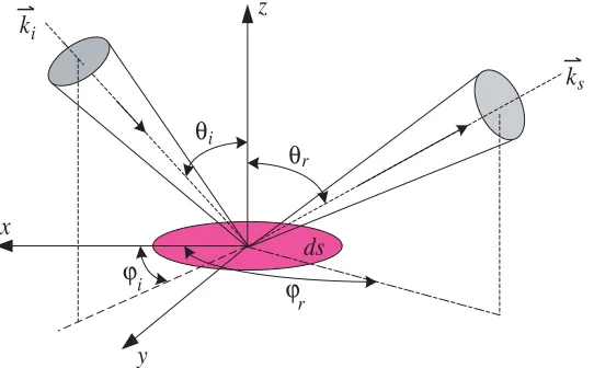
Target reflection is a complex process that depends on the target surface characteristics and the properties of the incident laser radiation. The BRDF quantifies all surface scattering characteristics. The definition of the BRDF [9, 10] of a differential surface is (see Figure 1)
fr(θi, ϕi, θr, ϕr) = dLr
(θi, ϕi, θr, ϕr) dEi(θi, ϕi)
(Sr−1) (1)
whereLr(θi, ϕi, θr, ϕr) is the radiance in the observation direction (θr, ϕr), andEi(θi, ϕi) is the incident
irradiance. The BRDF is expressed in the units of inverse steradians (Sr−1). The polarization can also be introduced into this expression.
ds x
z
y ki
s k
θ
ϕ
i
i
θr
ϕr
Figure 1. Geometry for the definition of the BRDF.
The analytical expressions for the BRDF, which are related to the surface parameters, are often too complex for practical use [11]. Here, we use the five-parameter BRDF statistical model [13], which is based on experimental data:
fr(θi, θr, ϕr) =kb k
2
rcosα
1 + (k2
r−1) cosα
exp[b(1−cosγ)a]G(θi, θr, ϕr)
cosθr +kd (2)
wherekb, kr, kd, a, bare the parameters to be determined. kr2cosα/[1 + (kr2−1) cosα] is the distribution
function for a micro-surface with a normal inclination ofα, exp[b(1−cosγ)] an approximate description of the Fresnel reflection coefficient, and G(θi, θr, ϕr) the flux reduction coefficient, which is introduced
to measure the effects of shadowing and masking. kb is the mirror reflection coefficient, kd the diffuse
coefficient, and θi, θr, ϕr are the angles of incidence, scattering angle and relative azimuth angle,
respectively. Here, ϕi = 0◦. In the following sections, a model optimized using the particle swarm
optimization algorithm based on limited experimental data is used [12, 13].
The relationship between the BRDF and the laser radar cross-section (LRCS) of a differential surface element can be derived [11] as follows.
wheredσis the LRCS of the differential surface areads. For a mono-static model, the LRCS is obtained by setting the illumination and observation angles to be equal, i.e.,
dσ= 4πfr(θ) cos2θds (4)
whereθ is the angle between the direction of incidence and the normal of the surface element.
2.2. Method of Analysis
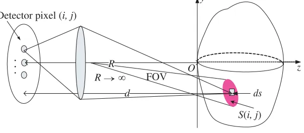
As shown in Figure 2, the laser pulse beam illuminates the target along thez-axis. For the mono-static configuration, the backscattering light ray is considered to propagate only parallel to thez-axis.
O
. .
.
ds
z y
FOV
Detector pixel (i, j)
S(i, j)
R R →∞
d
Figure 2. Schematic diagram of laser radar system.
The object surface is subdivided intoN small uncorrelated area elements denoted byAk, and the
contributions to the average irradiance at the receiver from each individual element are obtained based on the principles of radiometry [14], i.e.,
Ek= Wid2fr(θk) cos 2
θkAk (5)
where Ek is the irradiance in the observation direction, and Ai is the radiant flux density on the
target surface element after the transmitted beam has propagated by a distance d. This radiant flux density is a function of both time and the lateral position in the laser beam cross-section. Because the detector is assumed oriented perpendicularly to the z-axis, the radiant flux density on the detector is then equal to the irradiance. Each detector element in the two-dimensional array has a limited FOV (Figure 2), and thus the irradiance on each pixel is given by the contributions from the different points on a small surface area S within the FOV of the pixel. Because the N small areas are uncorrelated, the irradiance contributions from the different surface elements on the target are added incoherently without consideration of speckle effects [15]. The irradiance of a pixel is given by
Ei,j =
S(i,j)
Ek(t−t0−tk) (6)
where S(i,j) is the illuminated area corresponding to the FOV of the pixel (i, j), t0 = 2R/c the
round-trip propagation time of the laser pulse from the transceiver to the z= 0 plane (from which the object heighthk is defined), andtk = 2hk/c the round-trip propagation time between thez= 0 plane and the
k-th scattering cell.
3. SIMULATION AND ANALYSIS
target center (Figure 2). The radiant flux density of the laser beam propagating over a distance is still Gaussian [16]:
Wi(x, y, d) = 2P
πω2(d)exp
−2 r
2
ω2(d)
, r =x2+y2 (7)
where P is the transmitted power, d the scattering cell distance from the transmitter, and ω2(d) the
beam radius at a distance d. The temporal shape of the pulse power used in this case is also Gaussian:
P(t) =P0exp
−4πt2
τ2
(8)
where P0 is the peak power of the laser pulse and τ the full width at half maximum (FWHM) of the
pulse. Therefore, the irradiance of pixel (i,j) is obtained using Eqs. (5), (6), (7) and (8):
Ei,j =
S(i,j)
2P0
πω2(d)exp
−2 r
2
ω2(d)
exp
−4π(t−t0−tk)2
τ2
fr(θk) cos2θkAk
d2 (9)
This is the fundamental formula required for simulation of the laser radar 3D range imagery. The integration region S(i,j) is dependent on the distance to the target and the FOV of the pixel, which is
related to the active pixel area and the design of the receiver optics.
θ
(a) (b)
(c) 2
0 4 6 8 10 12
t/ns 1.0
0.8
0.6
0.4
0.2
0.0
Normalized intensity
τ = 0.3 ns
ρ = 1.0
θ = 0
θ = 45 o
o
3.1. Concepts of 3D Range Imagery
Figure 3 shows the simulation results obtained for a diffuse (Lambert) triconic, for which the BRDF is constant for different angles of incidence, i.e.,
fr= ρπ (10)
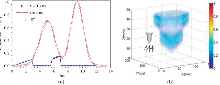
where ρ is the hemispherical reflectance. In the simulations, the peak power of the laser pulse is set at 106W; the FWHM of the laser pulse is 0.3 ns; the distance to the target is 10 km. To simplify the simulations, the FOV of a single pixel is set based on the pixel number for which the full FOV of the array detector just covers the target within the given range. As shown in Figure 3(a), the 1D LRP is different for various angles of incidence, which means that it can be used to provide feature vectors for ATR [17]. Figure 3(b) shows an orthographic view of the 3D range imagery of the triconic, which was stacked using 50 frames of slice images.
To reveal the spatial structure of the target more clearly, a computer rotated 3D representation of the image of Figure 3(b) and nine slice maps are shown in Figure 3(c). In the computer rotated 3D image, the triconic is displayed intuitively in Cartesian coordinates and color is used to represent the intensity. The upper half or the deeper part of the target is invisible after blanking. The slice maps reflect the evolution of the spatial structure in the longitudinal direction, and each 2D image corresponds to the intensity distribution on the array detector at a different time, with contributions from fractions of the target within a resolution cell at various ranges. The range resolution of this image is determined by the laser pulse width and FOVs of each of the pixels.
3.2. Effects of Pulse Width on Resolution of 3D Range Imagery
In 3D range imagery, each slice contains information about a girdle band in the target surface with a radial width of τ /2. In fact, the SPF of a single detector element is the 1D range profile of the target surface that is covered by the FOV of the pixel. According to 1D range profile theory [9], the convolution of a larger pulse width and larger target surface results in a larger reflected pulse width, which then induces lower range resolution in the detector response [11, 17].
Figure 4(a) shows the 1D LRPs of the triconic with an angle of incidence ofθ= 0◦(Figure 3), where the laser pulse widths are 0.3 ns and 4 ns. Here, the five-parameter BRDF statistical model is used in the simulations, and the values of kb, kr, and kd in Eq. (2) are set as 5.66, 2.34 and 0.23, respectively
(only three parameters are required for the backscattering model). When the pulse width is 0.3 ns, the profile of the backscattering signal envelope can reflect the target shape. However, at a larger pulse width of 4 ns, we cannot discriminate the cylindrical section of the triconic. The same situation occurs
(a) (b)
2
0 4 6 8 10 12
t/ns 1.0
0.8
0.6
0.4
0.2
0.0
Normalized intensity
τ = 0.3 ns
θ = 0o
14
τ = 4 ns
in 3D range imagery with a laser pulse width of 4 ns (Figure 4(b)). The target is shortened, and the middle section simply “vanishes”. In fact, the 3D range imagery with a large pulse width or when the temporal shape of the pulse is set to be constant is an intensity profile, similar to an image captured using a common charge-coupled device (CCD) camera.
3.3. Effects of Surface Material of Target on 3D Range Imagery
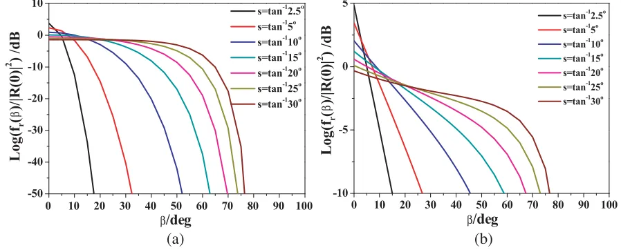
Because the BRDF of the Lambert sample is constant in Figure 3, the received intensity is solely dependent on the angle between the line of sight and the surface normal. As shown in Figure 3(b), as the angle between the line of sight and the surface normal decreases, the reflection intensity increases. However, in realistic situations, the scattering is a combination of both diffuse and specular components, and characterization of the scattering pattern is a sophisticated process. A more practical way to address this problem is to use a limited set of BRDF experimental data to predict the optical features of the materials. However, in the model used here, only the backscattered light is considered. To illustrate this concept, we use another two simple BRDF models derived from rough surfaces with slope density functions in Gaussian and exponential forms, respectively [18].
fr(β) = sec
6β
4πs2 exp
−tan2β
s2
|R(0)|2 (11)
fr(β) =
3 sec6β
4πs2 exp
−
√ 6 tanβ
s
|R(0)|2 (12)
wheres2 is the mean square slope of a two-dimensionally rough surface and R(0) the Fresnel reflection
coefficient for normal incidence. Curves for Eq. (11) and Eq. (12) for different values of sare shown in Figure 5.
0 10 20 30 40 50 60 70 80 90 100
-50 -40 -30 -20 -10 0 10 β/deg
s=tan-12.5o
s=tan-15o
s=tan-110o
s=tan-115o
s=tan-120o
s=tan-125o
s=tan-130o
Log( fr () /| R (0 )|
2 ) /d
B
0 10 20 30 40 50 60 70 80 90 100
-10 -5 0 5
s=tan-12.5o s=tan-15o s=tan-110o s=tan-115o s=tan-120o s=tan-125o s=tan-130o
Log (fr () /| R (0 )|
2 ) /d
B
(a) (b)
β/deg
β β
Figure 5. BRDF vs. incident angle for various root mean square slope of rough surfaces for two surface slope probability models. (a) Gaussian slope probability. (b) Exponential slope probability.
45
45
(a) (b) (c)
(d) (e) (f)
o
o
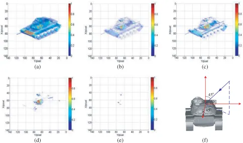
Figure 6. Effects of surface material of target on the 3D imagery. (a) Lambertian. (b) Exponential, where s = tan 30◦. (c) Gaussian, where s= tan 30◦. (d) Gaussian, where s= tan 20◦. (e) Gaussian, wheres= tan 5◦. (f) Open-GL model of the tank and the incident direction of the laser pulse.
mean square slopes are used. As shown in Figures 6(d) and (e), when the mean square slope is small, the imagery becomes obscure. In the latter case in particular, the tank is almost invisible.
4. CONCLUSIONS
Here we have developed a backscattering model of the received power in laser radar 3D range imagery based on the principle of radiometry. Using alternative mono-static BRDF models, simulations of the 3D range imagery of complex objects were performed. The effects of the target shape, surface material of target, laser pulse properties and angle of incidence on the range imagery were analyzed. The direct-detection model may be useful in ATR for space applications.
Because of the coherence of the laser light and the surface roughness on the scale of the optical wavelength, speckle effects will appear in the actual image. This model lays a foundation for the development of laser speckle simulations related to the diffuse components of the BRDF for laser radar imaging applications. Statistical analysis of the laser radar imaging system will be necessary for developing a more accurate model that incorporates these speckle effects, and this will form an important part of the next phase of this project.
ACKNOWLEDGMENT
REFERENCES
1. Heinrichs, R. M., B. F. Aull, and R. M. Marino, “Three-dimensional laser radar with APD arrays,” Proc. SPIE, Vol. 4377, 106–117, 2001.
2. Marius, B. F. A., A. Albota, and D. G. Fouche, “Three-dimensional imaging laser radars with geiger-mode avalanche photodiode arrays,” Lincoln Laboratory Journal, Vol. 13, No. 2, 351–370, 2002.
3. Marino, R. M., T. Stephens, and R. E. Hatch, “A compact 3D imaging laser radar system using Geiger-mode APD arrays: System and measurements,” Proc. SPIE, Vol. 5086, 1–15, 2003.
4. Richmond, R., “Laser radar focal plane array for three-dimensional imaging,”Proc. SPIE, Vol. 2748, 61–67, 1996.
5. Wang, J. and J. Kostamovaara, “Radiometric analysis and simulation of signal power function in a short-range laser radar,” Appl. Opt., Vol. 33, No. 18, 4069–4076, 1994.
6. Li, Y. H., Z. S. Wu, and Y. J. Gong, “Ultra-short pulse laser one-dimensional range profile of a cone,” Nucl. Instr. and Meth. A, 2010, doi:10.1016/j.nima.2010.02.044.
7. Gong, Y. J., Z. S. Wu, M. J. Wang, and Y. H. Cao, “Laser backscattering analytical model of Doppler power spectra about rotating convex quadric bodies of revolution,” Optics and Lasers in Engineering, Vol. 48, 107–113, 2010.
8. Li, Y. and Z. Wu, “Targets recognition using sub-nanosecond pulse laser range profiles,” Optics Express, Vol. 18, No. 16, 16788–16796, 2010.
9. Nicodemus, F. E., “Reflectance nomenclature and directional reflectance and emissivity,” Applied Optics, Vol. 9, No. 6, 1474–1475, 1970.
10. Stover, J. C., Optical Scattering Measurement and Analysis, McGraw-Hill, Inc., 1990.
11. Ove, S. and C. Tomas, “Three-dimensional laser radar modeling,” Proc. SPIE, Vol. 5412, 23–34, 2001.
12. Zhang, H., Z. Wu, Y. Cao, and G. Zhang, “Measurement and statistical modeling of BRDF of various samples,” Optica Applicata, Vol. XL, No. 1, 197–208, 2010.
13. Cao, Y. and Z. Wu, “Application of particle swarm optimization algorithms to parameter optimization of BRDF model,” Chinese Journal of Radio Science, Vol. 23, No. 4, 765–768, 2008. 14. Shirley, L. and G. Hallerman, “Applications of tunable lasers to laser radar and 3D imaging,”
Lincoln Laboratory, Massachusetts Institute of Technology, 1996.
15. Goodman, J. W., Speckle Phenomena in Optics: Theory and Applications, Roberts & Company, 2006.
16. Bury, E. V., “Synthesis of an object recognition system based on the profile of the envelope of a laser pulse in pulsed lidars,” Quantum Electronics, Vol. 28, No. 5, 458–462, 1998.
17. Cho, P., H. Anderson, R. Hatch, and P. Ramaswami, “Real-time 3D ladar imaging,” Lincoln Laboratory Journal, Vol. 16, No. 1, 147–164, 2006.