Dynamics and Stiffness Analysis of a Homopolar Magnetic Bearing
Xiaojun Ren1, *, Jinji Sun2, and Cunxiao Miao1
Abstract—Decreasing eddy current is very important for the realization of stability control of HoMB system. In order to improve the dynamic performance precision of HoMB in the design stage, the dynamics and stiffness analysis of a homopolar magnetic bearing (HoMB) has been studied in this paper. Because the polarities of the magnetic poles were not changed during the rotation of rotor, the effect of eddy-currents was often ignored in the previous researches. However, when the frequencies of vibration caused by external disturbance and control currents are very high, eddy-current effects have significant influence on the performance of HoMB. In order to predict the HoMB performance, guide the HoMB design and control of the HoMB system in high frequency, a dynamics model was built on the equivalent circuit method. Parameters of dynamic Modeling are frequency-dependent. The effect of eddy-currents on the current stiffness was studied. The analysis results show that the eddy current effect on HoMB can be reduced by increasing the air gap, decreasing the laminations thickness and decreasing the laminations conductivity.
1. INTRODUCTION
Due to the advantages of no friction, no abrasions, no lubrication, no maintenance, high speed, high precision, etc. [1–4], magnetic bearings (MB) have been widely applied in reaction wheels, energy storage flywheels [5, 6], control momentum gyros [7], momentum wheels, high reliability compressors [8], molecular vacuum pumps [9], and robotics [10, 11] among others.
Generally, radial MBs can be divided into two categories based on the magnetic polarities seen by rotor as it rotates [17]. One is HoMB, and the other is heteropolar magnetic bearing. Compared to the heteropolar magnetic bearing, homopolar magnet structures have much lower rotational losses because of less field variation of rotor and lower induced eddy currents [18–21]. Since the polarities of the magnetic poles were not changed during the rotation of rotor, the effect of eddy-currents was often ignored in previous studies. However, when the frequencies of vibration caused by external disturbance and control currents are very high, eddy-current effects have significant influence on the performance of HoMB.
Due to the time-varying magnetic field, eddy currents exist in the stator and rotor of MBs as the rotor rotates [22–25]. In [22], the authors analyzed the eddy-current loss for design of small active magnetic bearings with solid core and rotor. Due to the high rotational speeds, eddy current losses became lager. In [23], the eddy current losses in the thin surface layer of a laminated core were analyzed. Besides, eddy current reduces force of actuator and cause the phase lag between actuator coil current and the force. The magnetic field would be weaken by eddy currents [24, 25]. In [25], a new method for analyzing the eddy current fields in laminations is presented. This method was based on the equivalent conductivity and permeability. All these effects are very important to the performance of control system. However, the dynamic stiffness of the magnetic bearing decreases at high speed.
Received 15 September 2018, Accepted 28 November 2018, Scheduled 13 December 2018 * Corresponding author: Xiaojun Ren ([email protected]).
Research on the stiffness of the existing literature on homopolar magnetic bearing usually adopts static stiffness value.
This paper focuses on the dynamics and stiffness analysis of a HoMB. By establishing the dynamic magnetic circuit model of magnetic bearing, the expression of dynamic stiffness is derived. The theoretical analysis curve of dynamic stiffness is analyzed. The influence of key design parameters on dynamic stiffness is obtained through simulation analysis. A test method of dynamic stiffness is put forward, and experiments are carried out on the prototype. Finally, the test values are compared with the previous theoretical values, and conclusion is given out.
In order to predict the performance and guide the design of the HoMB drive in high frequency for controlled in vacuum environments, for small amplitude high frequency disturbances of the equilibrium position, the influence of displacement stiffness on the dynamic performance is much less than that of the control current. Therefore, the stiffness analysis of this paper is mainly aimed at the analysis of dynamic current stiffness. Firstly, structure and model of HoMB were briefly introduced. Secondly, dynamic modeling has been deduced. Thirdly, effects of key parameters on the dynamic performance were analyzed. Finally, distribution of magnetic fields, eddy current loss and frequency response of current stiffness were analyzed by FEM.
2. STRUCTURE OF HOMB
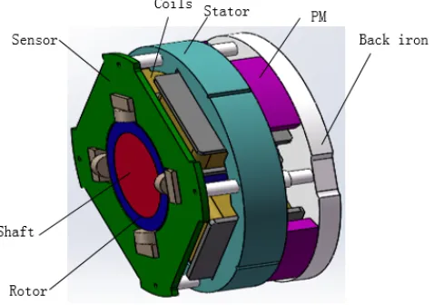
The structure of the HoMB to be analyzed in this paper is shown in Fig. 1. This four-pole HoMB consists of a radial stator, a rotor, a shaft, permanent magnets and a back iron. The magnetic poles are wound with coils. A displacement sensor circuit board is installed next to the radial stator. Four displacement sensors are mounted on the circuit board to detect the displacement of rotor. Compared to a two-stator and eight-pole structure, this HoMB has shorter axial length. Bias magnetic flux was provided by four separated permanent magnets instead of bias current. Usually, the static working point determined by the permanent magnets is set as half of saturated magnetic density of material. Difference control method was applied to the control current. When the HoMB works, for one radial air gap between the stator and rotor, the control flux will be added together with the bias flux, whereas in the radial air gap of opposite direction, the control flux will be subtracted from the bias flux. As a result, the difference of magnetic flux between these two air gaps generates magnetic levitation force to keep the rotor balance.
Figure 1. Structure of the HoMB to be analyzed in this paper.
3. DYNAMIC MODELING
position. But when dynamic load occurs, the current in the coil will appear in the corresponding frequency to keep the rotor stable. For this situation, the eddy current effect cannot be ignored.
3.1. Dynamic Permeability
For a HoMB, Maxwell’s equations for time-varying magnetic field can be written as
∇ ×E = −∂B
∂t (1)
∇ ×H = J (2)
∇ ·B = 0 (3)
whereE is the electric field intensity;B is the magnetic flux density; H is the magnetic field intensity; J is the current intensity.
Constitutive relation of medium material can be expressed as
B = μ0μrH (4)
J = σE (5)
where μ0 is the permeability of vacuum; μr is the relative permeability of material; σ is the electronic conductivity.
Combining Eqs. (1), (2), (3), (4) and (5), the following can obtained
∇2B =σμ 0μr
∂B
∂t (6)
Ignore end effects and assume that all magnetic field lines are perpendicular to the surface of the rotor and the surface of magnetic pole. Then, magnetic field in the air gap does not have axial component. It means that magnetic field between rotor and stator has onlyx and y components.
For laminated plates, the change of B in the z direction is much larger than that in the radial direction. Therefore, the change ofB in the radial direction can be ignored.
∂B ∂x = 0;
∂B
∂y = 0 (7)
Therefore, Eq. (6) can be changed into
∂2B
∂z2 =σμ0μr ∂B
∂t (8)
HereB can be expressed in complex number
B =Bn0(x, y)ejwt (9)
Substituting Eq. (9) into Eq. (8) for the same part, we can get
∂2B
∂z2 −jωσμ0μrB = 0 (10)
Solving this equation, we can get the expression of general solution as follows
B =c1eλz+c2e−λz (11)
whereλis the eigenvalue; c1 and c2 are the undetermined coefficients.
λ=jωσμ0μr (12)
According to the continuity of magnetic field strength, we can get boundary conditions of the outer surface and inner surface of the rotor.
For Eq. (9), defineBn0x and Bn0y as the components in the x andy directions, respectively, then
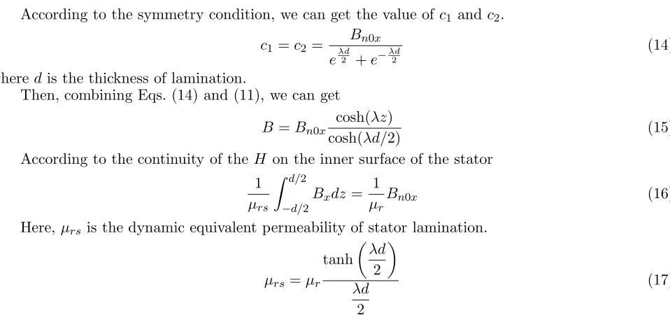
According to the symmetry condition, we can get the value ofc1 andc2.
c1 =c2 =
Bn0x
eλd2 +e−λd2
(14)
wheredis the thickness of lamination.
Then, combining Eqs. (14) and (11), we can get
B=Bn0x
cosh(λz)
cosh(λd/2) (15)
According to the continuity of theH on the inner surface of the stator
1 μrs
d/2
−d/2
Bxdz= 1 μr
Bn0x (16)
Here,μrs is the dynamic equivalent permeability of stator lamination.
μrs=μr tanh
λd 2
λd 2
(17)
3.2. Analysis of PM Bias Circuits
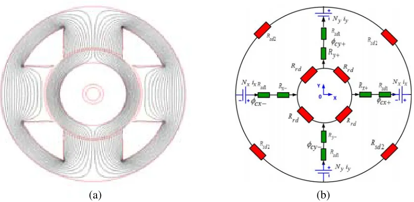
Figure 2(a) shows the bias flux path generated by the permanent magnet. Fig. 2(b) shows its equivalent magnetic circuit model.
(b) (a)
Figure 2. Section view of the HoMB and its equivalent magnetic circuit. (a) Cross-section of bias flux. (b) Equivalent magnetic circuit.
Considering the relative small displacement compared with the dimension of the stator air gap, we can assume that the air gap reluctance between the back iron and the rotor can be simplified as constant valueRir under acceptable tolerance. In the following analysis we will validate this assumption. Then, we can define
Rp=Rpm+Rir (18)
where Rpm is the reluctance of permanent magnet; Rir is the reluctance of air-gap between the rotor and back iron.
Rx+, Rx−, Ry+ and Ry− are the reluctances of air-gap in x+, x−, y+ and y− directions, respectively. Reluctance of the radial air gap can be calculated as
Rrg = gr μ0Ar
wheregr is the length of radial air gap; Ar is the area of the pole;
Based on the Kirchhoff’s law in magnetic circuit, according to Fig. 2(b), we can get magnetic circuit
equations: ⎡ ⎢ ⎢ ⎢ ⎢ ⎢ ⎣
Rp Rx+
Rp Rx−
Rp Ry+
Rp Ry−
1 −1 −1 −1 −1
⎤ ⎥ ⎥ ⎥ ⎥ ⎥ ⎦ ⎡ ⎢ ⎢ ⎢ ⎢ ⎢ ⎣ φpm φpx+ φpx− φpy+ φpy−
⎤ ⎥ ⎥ ⎥ ⎥ ⎥ ⎦ = ⎡ ⎢ ⎢ ⎢ ⎢ ⎣ Fpm Fpm Fpm Fpm 0 ⎤ ⎥ ⎥ ⎥ ⎥ ⎦ (20)
where φpm is the bias flux of the stator magnetic yoke; φpx+, φpx−,φpy+ and φpy− are the bias fluxes of air-gap in x+, x−, y+ and y− directions, respectively; magnetomotive force (MMF) Fpm can be calculated as
Fpm=Hpmlpm (21)
In the above expression,Hpm is the coercive force; lpm is the magnetization length. By solving the matrix equation (20), we get every magnetic flux as follows:
⎡ ⎢ ⎢ ⎢ ⎢ ⎢ ⎣ φpm φx+ φx− φy+ φy−
⎤ ⎥ ⎥ ⎥ ⎥ ⎥ ⎦ = ⎡ ⎢ ⎢ ⎢ ⎢ ⎢ ⎢ ⎢ ⎢ ⎢ ⎢ ⎢ ⎢ ⎢ ⎢ ⎢ ⎣
FpmG (1 +RpG)
1 Rx+
Fpm (1 +RpG) 1
Rx−
Fpm (1 +RpG) 1
Ry+
Fpm (1 +RpG) 1
Ry−
Fpm (1 +RpG)
⎤ ⎥ ⎥ ⎥ ⎥ ⎥ ⎥ ⎥ ⎥ ⎥ ⎥ ⎥ ⎥ ⎥ ⎥ ⎥ ⎦ (22) where ⎧ ⎪ ⎪ ⎨ ⎪ ⎪ ⎩
G= 1
Rx+ + 1
Rx− + 1
Ry+ + 1
Ry−
Rx+= g0+x
μ0A
, Rx−= g0−x
μ0A
, Ry+= g0+y
μ0A
, Ry−= g0−y
μ0A
(23)
When the rotor is located at original, displacement x= 0 andy = 0,
⎡ ⎢ ⎢ ⎢ ⎢ ⎢ ⎣ φpm φx+ φx− φy+ φy−
⎤ ⎥ ⎥ ⎥ ⎥ ⎥ ⎦
= AFmμ0 g0+ 4ARpμ0
⎡ ⎢ ⎢ ⎢ ⎢ ⎢ ⎣ 4 1 1 1 1 ⎤ ⎥ ⎥ ⎥ ⎥ ⎥ ⎦ (24)
3.3. Dynamic Control Circuit Model
When the frequency of current is low, the eddy current effect of magnetic bearing performance influence is weak. In this case, the traditional static magnetic circuit model is feasible for the analysis of magnetic bearing performance. Static magnetic circuit model ignores the reluctance of iron and only calculates the air gap reluctance. When the magnetic bearings are applied to high speed, the eddy current generated by the high frequency dynamic electromagnetic field will affect the performance of magnetic bearing, which will result in the decrease of magnetic force and the lag of phase. Therefore, the eddy current effect must be taken into account, including the static magnetic circuit model of the dynamic magneto resistance.
When the rotor is located in balanced position
(b) (a)
Figure 3. Plot of dynamic control magnetic circuit. (a) Magnetic flux path. (b) Equivalent magnetic circuit.
Using superposition method, when the current is only in the coil ofx+ direction, the total magnetic resistance of control magnetic flux can be expressed
Rctotal=Rsd2+ 2Rsd1+ 2Rrg+Rrd (26)
whereRsd1 and Rsd2 are equivalent dynamic magnetic resistance of the corresponding stator iron core; Rrd is the equivalent dynamic magnetic resistance of rotor.
Figure 4. Plot of magnetic circuit of paired-pole configuration.
According to Eq. (17) and geometric parameter shown in Fig.4, we can get
Rsd1 =
π(r4+r3) 4μ0μdyl1(r4−r3)
(27)
Rsd2 = 1 μ0μdyA
r4+r3
2 −r2−g
(28)
Rrd =
r1+r2 4μ0μdyl(r2−r1)
(29)
The magnetic flux through the x+ direction magnetic pole is
φcx+= Nxix Rctotal
Therefore, with thex+ andx−directions of magnetic poles at the same time, the direction of the magnetic pole in the atmosphere of the total control of the magnetic flux
φc = 2Nxix Rctotal
(31)
If the load is static, the control current is DC current. The core resistance and rotor resistance can be neglected. So Eq. (31) can be changed into
φstc = Nxix Rrg
(32)
3.4. The Deduction of the Electromagnetic Force and Stiffness
When the rotor is at the equilibrium position, bias magnetic flux is superimposed by the control flux. The electromagnetic suspending force inx-direction generated by the magnetic bearing can be expressed as
Fx = 1 2μA
(φx++φc)2−(φx−−φc)2
(33)
When the load is static, the control current is DC current. Then we substitute Eqs. (22) and (33) for the same parameters in Eq. (35), resulting in the expression changed into
Fxst= 2FmNxix μ0Rrg(4ARpμ0μr−g0)
(34)
As we have analyzed the electromagnetic force by First-order Taylor Series Expansion for simple cases in Eq.(35), the electromagnetic force in x-axis direction and y-axis direction can be expressed as the follows:
F(x, ix)∼= ∂F ∂ix
ix = 0 x= 0
ix+ ∂F
∂x
ix= 0 x= 0
x=kixix+kdxx (35)
Therefore, the static force-current factor inx-direction can be deduced through Eqs. (36) and (37)
kix = ∂F ∂ix
ix = 0 x= 0
= 4FmNxix
μ0Rctotal(4ARpμ0+g0)
(36)
The static force-displacement factor inx-direction can be deduced through Eqs. (36) and (37)
kdx= −
4FmNxix μ0Rctotal(4ARpμ0+g0)2
(37)
When the load is dynamic, control flux can be expressed as
φACc (jω) = 2Nxi0e jωt
Rctotal
(38)
The dynamic force-current factor in x-direction can be deduced through Eqs. (35) and (40).
G(jω) = Fx(jω) i0ejωt
= 4FmNx
μ0(Rsd2+ 2Rsd1+ 2Rrg+Rrd)(4ARpμ0+g0)
(39)
Amplitude-frequency characteristic can be expressed as
M(ω) = 20 logG(jω) G(0)
(40)
Phase-frequency characteristic can be expressed as
P a(ω) =∠
G(jω) G(0)
4. EFFECTS OF KEY PARAMETERS ON THE DYNAMIC PERFORMANCE 4.1. Length of Air-Gap
Eqs. (17),(24) and (41) show that the air gap is a critical parameter to the dynamic current stiffness. Fig. 5 shows the effect of air gap length on the magnitude and phase of current stiffness at different frequencies. The higher the frequency is, the greater the attenuation of amplitude and frequency is. It can be seen that when the length of the air gap increases, magnitude attenuation degree and phase delay of current stiffness decrease quickly at first and then slow down.
0.1 0.2 0.3 0.4 0.5 0.6 0.7 0.8 0.9 1 -2.5
-2 -1.5 -1 -0.5 0
Length of air-gap(mm)
A
m
pl
it
ude (
d
B
) 100 Hz
500 Hz 1000 Hz 1500 Hz
0 0.1 0.2 0.3 0.4 0.5 0.6 0.7 0.8 0.9 11 -14
-12 -10 -8 -6 -4 -2 0
Length of air-gap(mm)
P
hase (
deg)
100 Hz
500 Hz
1000 Hz
1500 Hz
(b) (a)
Figure 5. Current stiffness varies with the air gap at different frequencies. (a) Magnitude. (b) Phase.
5. THE THICKNESS OF LAMINATIONS
Figure 6 shows the effect of the thickness of laminations on the current stiffness. It can be seen that decreasing the thickness of laminations can decrease the magnitude attenuation degree and phase delay of current stiffness.
0.1 0.2 0.3 0.4 0.5
-2.5 -2 -1.5 -1 -0.5 0
Thickness of lamination(mm)
A
m
pl
it
ude (
d
B
)
100 Hz
500 Hz
1000 Hz
1500 Hz
0.1 0.2 0.3 0.4 0.5
-12 -10 -8 -6 -4 -2 0
Thickness of lamination(mm)
P
h
ase (
d
eg)
100 Hz
500 Hz
1000 Hz
1500 Hz
(b) (a)
6. CONDUCTIVITY OF MATERIALS
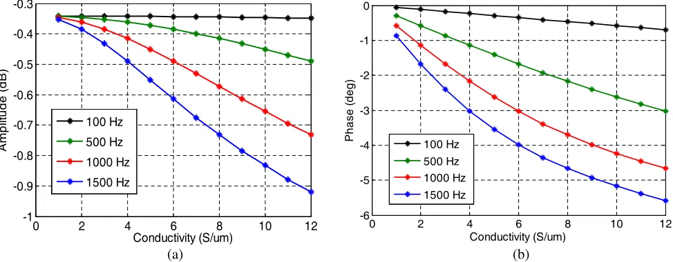
Figure 7 shows the effect of the conductivity of laminations on the current stiffness. It can be seen from Fig. 7 that decreasing the conductivity of materials can decrease the magnitude attenuation degree and phase delay of current stiffness. Compared to Fig. 6, it can be seen that the effect of conductivity on current stiffness is not as obvious as that of thickness of laminations.
0 2 4 6 8 10 12
-1 -0.9 -0.8 -0.7 -0.6 -0.5 -0.4 -0.3
Conductivity (S/um)
Am
p
lit
u
d
e
(
d
B)
100 Hz
500 Hz
1000 Hz
1500 Hz
0 2 4 6 8 10 12
-6 -5 -4 -3 -2 -1 0
Conductivity (S/um)
P
h
ase (
d
eg)
100 Hz
500 Hz 1000 Hz 1500 Hz
(b) (a)
Figure 7. Current stiffness varies with conductivity of laminations at different frequencies. (a) Magnitude. (b) Phase.
7. FEM ANALYSIS
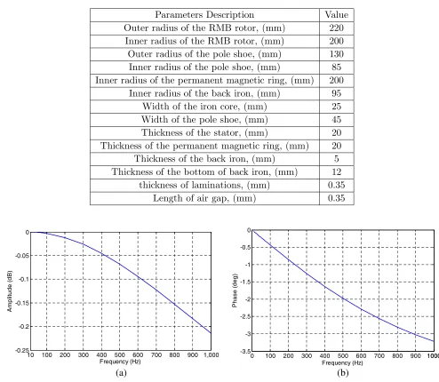
The values of main parameters of HoMB are listed in Table 1. The distribution of magnetic flux density of HoMB is calculated by Maxwell Ansoft with 3-D model, while the results are shown in Fig. 8 in 2-D view. Bias flux density was designed as 0.6 T, half of saturation value.
(b)
(a) (c)
Figure 8. Distribution of magnetic flux density. (a) Axial section view. (b) Back face view. (c) Front face view.
Table 1. Values of main parameters of HoMB.
Parameters Description Value Outer radius of the RMB rotor, (mm) 220
Inner radius of the RMB rotor, (mm) 200 Outer radius of the pole shoe, (mm) 130 Inner radius of the pole shoe, (mm) 85 Inner radius of the permanent magnetic ring, (mm) 200
Inner radius of the back iron, (mm) 95 Width of the iron core, (mm) 25 Width of the pole shoe, (mm) 45 Thickness of the stator, (mm) 20 Thickness of the permanent magnetic ring, (mm) 20 Thickness of the back iron, (mm) 5 Thickness of the bottom of back iron, (mm) 12
thickness of laminations, (mm) 0.35 Length of air gap, (mm) 0.35
10 100 200 300 400 500 600 700 800 900 1,000 -0.25
-0.2 -0.15 -0.1 -0.05 0
Frequency (Hz)
A
m
pl
it
ude (
d
B
)
0 100 200 300 400 500 600 700 800 900 10001000 -3.5
-3 -2.5 -2 -1.5 -1 -0.5 0
Frequency (Hz)
P
h
ase (
deg)
(b) (a)
Figure 9. Frequency response of current stiffness. (a) Magnitude. (b) Phase.
8. CONCLUSION
This paper introduces the dynamics and stiffness analysis method of a hybrid HoMB including eddy currents. For the HoMB, the eddy currents are mainly caused by time-varying control currents. The dynamics model is built on the equivalent circuit method. The induced eddy currents will result in the magnitude decrease and phase delay of the dynamic stiffness, which is very important for the control. Analysis results show that the eddy current effect on HoMB can be reduced by increasing the air gap, decreasing the laminations thickness and decreasing the laminations conductivity.
ACKNOWLEDGMENT
REFERENCES
1. Eaton, D., J. Rama, and S. Singhal, “Magnetic bearing applications & economics,” Proc. PCIC, 1–9, Sep. 2010.
2. Xu, S. L. and J. C. Fang, “A novel conical active magnetic bearing with claw structure,” IEEE Transactions on Magnetics, Vol. 50, No. 5, 8101108, 2014.
3. Ren, X. J., Y. Le, J. J. Sun, et al., “Magnetic flux leakage modeling and optimization of a combined radial-axial hybrid magnetic bearing for DC motor,” IET Electric Power Applications, DOI: 10.1049/iet-epa.2016.0259, to be published.
4. Huang, Z., J. Fang, X. Liu,, and B. Han, “Loss calculation and thermal analysis of rotors supported by active magnetic bearings for high-speed permanent magnet electrical machines,”
IEEE Transactions on Industrial Electronics, Vol. 63, No. 4, 2027–2035, 2016.
5. Bai, J. G., X. Z. Zhang, and L. M. Wang, “A flywheel energy storage system with active magnetic bearings,”Proc. 2012 Int. Conf. Future Energy, Environ., Mater., Vol. 16, 1124–1128, pt. B, 2012. 6. Tang, J., J. J. Sun, J. C. Fang, et al., “Low eddy loss axial hybrid magnetic bearing with gimballing control ability for momentum flywheel,” Journal of Magnetism & Magnetic Materials, Vol. 329, No. 2, 153–164, 2013.
7. Fang, J. C., S. Q. Zheng, and B. C. Han, “AMB vibration control for structural resonance of double-gimbal control moment gyro with high-speed magnetically suspended rotor,”IEEE/ASME Transactions on Mechatronics, Vol. 18, No. 1, 32–43, 2013.
8. Fang, J., Y. Le, J. Sun, and K. Wang, “Analysis and design of passive magnetic bearing and damping system for high-speed compressor,” IEEE Transactions on Magnetics, Vol. 48, No. 9, 2528–2537, 2012.
9. Noh, M. D., S. Cho, J. Kyung, S. Ro, and J. Park, “Design and implementation of a fault-tolerant magnetic bearing system for turbo molecular vacuum pump,”IEEE/ASME Transactions on Mechatronics, Vol. 10, No. 6, 626–631, 2005.
10. Gilchrist, U., M. Hosek, J. T. Moura, et al., “Robot drive with magnetic spindle bearings,” USA Patent, US20090243413 A1, 2009.
11. Hollis, Jr., R. L., “Magnetically levitated fine motion robot wrist with programmable compliance,”
USA Patent, US4874998 A, 1987.
12. Beniak, R. and T. Pyka, “An energy-consumption analysis of a tri-wheel mobile robot,” International Journal of Robotics and Automation, Vol. 31, No. 1, 2016, DOI: 10.2316/Journal.206.2016.1.206-4079.
13. Liang, L., P. Tang, and B. Chen, et al., “Dynamical modelling and structural parameter optimization of a novel spiral in-pipe robot,” International Journal of Robotics and Automation, Vol. 31, No. 1, 2016, DOI: 10.2316/Journal.206. 2016.1.206-4170.
14. Zhu, Y., X. Sun, and X. Wang, “Locomotion system design and dynamics analysis of a new telescopic miniature in-pipe robot,” International Journal of Robotics and Automation, Vol. 31, No. 2, 2016, DOI: 10.2316/Journal.206.2016.2.206-4361.
15. Higuchi, T., K. Oka, and H. Sugawara, “Clean room robot with noncontact joints using magnetic bearings,” Advanced Robotics, Vol. 7, No. 2, 105–119, 1993.
16. Selmy, M., M. Fanni, and A. M. M. Mohamed, “Design and control of a novel contactless active robotic joint using AMB,” 2015 IEEE International Conference on Autonomous Robot Systems and Competitions (ICARSC), 144–149, Dec. 2015, DOI: 10.1109/ICARSC.
17. Schweitzer, G. and E. H. Maslen, Magnetic Bearings Theory, Design and Application to Rotating Machinery, Springer-Verlag, Berlin, 2009.
18. Zhang, W. and H. Zhu, “Improved model and experiment for AC-DC three-degree-of-freedom hybrid magnetic bearing,”IEEE Transactions on Magnetics, Vol. 49, No. 11, 5554–5565, 2013. 19. Fang, J. C., et al., “Homopolar 2-pole radial permanent-magnet biased magnetic bearing with low
20. Eryong, H. and L. Kun, “A novel structure for low-loss radial hybrid magnetic bearing,” IEEE Transactions on Magnetics, Vol. 47, No. 12, 4725–4733, 2011.
21. Kim, H.-Y. and C.-W. Lee, “Analysis of eddy-current loss for design of small active magnetic bearings with solid core and rotor,” IEEE Transactions on Magnetics, Vol. 40, No. 5, 3293–3301, 2004.
22. Muramatsu, K., T. Shimizu, A. Kameari, I. Yanagisawa, S. Tokura, O. Saito, and C. Kaido, “Analysis of eddy currents in surface layer of laminated core in magnetic bearing system using leaf edge elements,” IEEE Transactions on Magnetics, Vol. 42, No. 4, 883–886, 2006.
23. Tian, Y., Y. Sun, and L. Yu, “Modeling of switching ripple currents (SRCs) for magnetic bearings including eddy current effects,” International Journal of Applied Electromagnetics and Mechanics, Vol. 33, 791–799, 2012.
24. Wang, J., H. Lin, Y. Huang, and L. Huang, “Numerical analysis of 3D eddy current fields in laminated media under various frequencies,” IEEE Transactions on Magnetics, Vol. 48, No. 2, 267–270, 2012.