Wind Loading on Full-scale Solar Panels

(1)

Scholarship@Western

Electronic Thesis and Dissertation Repository

2-8-2016 12:00 AM

Wind Loading on Full-scale Solar Panels

Zeinab Samani

The University of Western Ontario

Supervisor Horia Hangan

The University of Western Ontario Joint Supervisor Girma Bitsuamlak

The University of Western Ontario

Graduate Program in Civil and Environmental Engineering

A thesis submitted in partial fulfillment of the requirements for the degree in Master of Science © Zeinab Samani 2016

Follow this and additional works at: https://ir.lib.uwo.ca/etd

Part of the Civil and Environmental Engineering Commons

Recommended Citation Recommended Citation

Samani, Zeinab, "Wind Loading on Full-scale Solar Panels" (2016). Electronic Thesis and Dissertation Repository. 3529.

https://ir.lib.uwo.ca/etd/3529

This Dissertation/Thesis is brought to you for free and open access by Scholarship@Western. It has been accepted for inclusion in Electronic Thesis and Dissertation Repository by an authorized administrator of

(2)

Wind load governs the design of supporting structures of solar panels and constitutes

approximately fifty percent of the total cost. There are various test scale related issues while

testing solar panels (small structures) in boundary layer wind tunnel laboratories meant for tall

buildings (large structures). Emergence of large testing facilities, however, is enabling testing

full-scale solar panels. In this thesis an extensive experimental program is conducted at

WindEEE Dome using full-scale solar panels and finite element modeling. The experimental

program includes: (i) high resolution pressure tests to understand the sensitivity of pressure

taps density and distribution; (ii) force balance test to determine the reactions of the solar panel

under wind loading accounting for aeroelastic effects and validate pressure test results; (iii)

finite element modeling to assess the internal stress of the solar rack elements and improvement

of the rack cross section.

Study of pressure tap layout and resolution illustrated that a fairly high density resolution is

required to capture all the aerodynamic features of pressure on the solar panel surfaces. It is

found that the uplift force obtained from the force balance tests are larger compared to the

pressure taps as result of the dynamic effects of wind loading. The finite element analysis of

solar racks was performed using the experimentally established wind loading data, which

includes all dynamic features of the forces obtained from the force balances. It is concluded

that the solar rack cross sections can be structurally optimized and there is a possibility to save

in aluminum elements up to 40%.

Keywords

Full-Scale Solar Panel, Experimental Analysis, Wind Testing, WindEEE Dome, Finite

(3)

ii

Co-Authorship Statement

This thesis has been produced in accordance with the guidelines of the School of Graduate and

Postdoctoral Studies. All the experiments, numerical modeling, calibration, interpretation of

results and writing the draft and final version of thesis were carried out by the candidate herself,

under the supervision of Prof. Horia Hangan and Prof. Girma Bitsuamlak. The supervisors’

contribution consisted of providing advice throughout the research program and reviewing the

(4)

iii

Acknowledgments

I would like to express my appreciation to the people who have supported me through this

research and have been essential to its completion.

I am extremely thankful and indebted to my supervisors Prof. Horia Hangan and Prof. Girma

Bitsuamlak who have been invaluable in providing assistance, guidance and recommendations

along the way. Their constant technical and motivational supports were unforgettable for me.

Sincere thanks to the manager of German Solar Corporation, Mr. Dennis German, for

providing the opportunity and funding of this interesting project.

I am so grateful to employees and fellows of the WindEEE Gerry Dafoe, Andrew Mathers, and

Adrian Costache and Dr. Maryam Refan, who have tirelessly assisted me in this project.

A special thanks to Dr. Ahmad Elatar and Dr. Chowdhury Mohammad Jubayer, Tibebu

Birhane who shared their feedback, guidance, assistance and support during this research.

I would like to thank my other friends and staff at the Wind Engineering, Energy and

Environment (WindEEE) Research Institute and Boundary Layer Wind Tunnel Laboratory for

their support especially Mahshid Nasiri, Djordje Romanic, Ryan Kilpatrick and Dan Parvu for

all their helps.

To my parents, for their unceasing encouragement, support and affections. I am proud to be

your daughter and fully indebted to you because of your dedications and self-sacrifice

throughout my life.

Last but certainly not the least, a great gratitude to my wonderful husband, Dr. Bahman Daee.

I will always remember how he helped me these years. Without his patience, understanding,

(5)

iv

List of Tables

Table 2.1: The experimental test cases in WindEEE ... 26

Table 2.2: Characteristic of the pressure test ... 27

Table 3.1: Reynolds number of boundary layer and uniform flow ... 44

Table 3.2: Peak pressure coefficient load case ... 45

Table 3.3: Drag force Coefficient obtained from ASCE and maximum Cp from experimental analysis for 0 degree wind angle of attack ... 46

Table 3.4: Validation and comparison wind induced drag force obtained from force balances and pressure taps ... 48

Table 3.5: Validation and comparison wind induced lift force obtained from force balances and pressure taps ... 49

Table 4.1: Section properties of P1000 uni-strut ... 54

Table 4.2: Engineering properties of aluminum 6061-T6 ... 55

Table 4.3: Steps to find the instant that the pressure achieved its peak value ... 56

Table 4.4: Comparison of FEA support reactions with the experimental results obtained from force balances for 20 kg point load ... 58

Table 4.5: Comparison of FEA reactions with the experimental results obtained from pressure model and force balances ... 59

Table 4.6: Capacity of P1000 uni-strut columns ... 62

(9)

viii

List of Figures

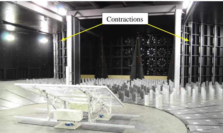
Figure 1.1: View of contractions at WindEEE Dome used for the experiments ... 3

Figure 1.2: Aerodynamic forces on an inclined flat plate ... 5

Figure 1.3: Tributary area of each taps ... 5

Figure 1.4: Typical view of roof-mounted solar panels ... 6

Figure 1.5: Typical view of ground-mounted solar panels ... 6

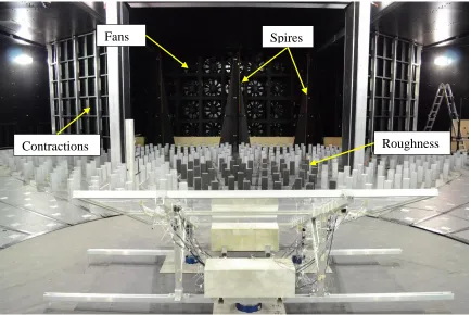
Figure 2.1: View of passive flow conditioning elements at WindEEE used for the experiments ... 14

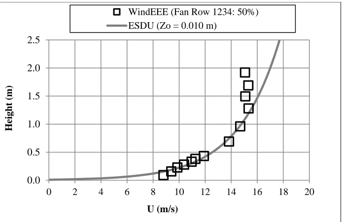
Figure 2.2: Comparison of mean wind velocity profile measured at WindEEE and ESDU standard for open terrain with Zo=0.01 ... 15

Figure 2.3: Comparison of mean turbulence intensity profile measured at WindEEE and ESDU standard for open terrain with Zo=0.01 ... 15

Figure 2.4: Comparison of spectra of stream-wise turbulence velocity measured at WindEEE and ESDU standard at the solar panel height, H=0.96 m ... 16

Figure 2.5: Pressure test model ... 17

Figure 2.6: Pressure test model set-up in WindEEE ... 18

Figure 2.7: Tap layout of a panel (a) upper surface (b) lower surface (127 pressure taps on each) ... 19

Figure 2.8: Aero-elastic model (full-scale solar panel) test set-up at WindEEE ... 20

Figure 2.9: Solar panel supporting structure, concrete ballasts and location of force balances ... 21

(10)

ix

Figure 2.11: Cobra Probe and Pitot tube set-up in WindEEE ... 23

Figure 2.12: View of the connection of vinyl tubes using brass connectors ... 24

Figure 2.13: Bottom view of solar model showing the vinyl tubes and scanners ... 24

Figure 2.14: Instrumentation of the test set-up in WindEEE ... 25

Figure 3.1: Mean and net pressure coefficient (Cp) contours on the panels for different wind angles of attack ... 29

Figure 3.2: (a) Mean, (b) maximum and (c) minimum equivalent pressure coefficient for all wind angles of attack ... 32

Figure 3.3: Comparison of mean net pressure coefficient of solar panel with 25o slope, a) 1:10 scale (Aly et al. 2012), b) full-scale model ... 33

Figure 3.4: Model configuration of present study and Abiola-Ogedengbe (2013) with 25o inclined panel at 0o wind angle of attack ... 34

Figure 3.5: Mean Cp profiles along the mid-line of the panel surface for wind angles of attack of 0o ... 35

Figure 3.6: Mean Cp profiles along the mid-line of the panel surface for wind angles of attack of 180o Figure ... 35

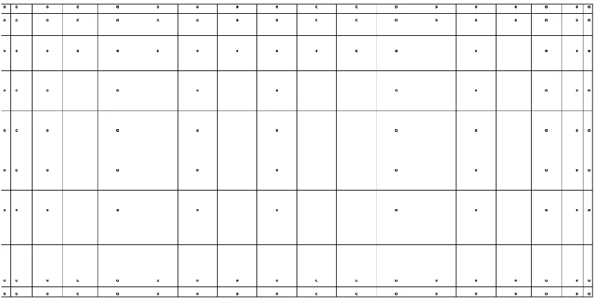
Figure 3.7: Pressure tap layout for four different resolutions ... 37

Figure 3.8: Net mean pressure coefficient (Cp) distribution of 0 degree wind angle of attack for different resolution ... 39

Figure 3.9: CPnet of different pressure tap layouts at 0 degree wind angle of attack ... 39

(11)

x

Figure 3.12: Net mean pressure coefficient (Cp) distribution of 135 degree wind angle of

attack for different resolution ... 41

Figure 3.13: CPnet of different pressure tap layout for 135 degree wind angle of attack ... 41

Figure 3.15: CPnet of different pressure tap layout for 180 degree wind angle of attack ... 42

Figure 3.16: Comparison of Cpnet contour plots obtained from boundary layer and uniform flow for 0 degree wind direction ... 43

Figure 4.1: Plan and section view of the solar panel supporting structure ... 53

Figure 4.2: Cross section geometry of P1000 uni-strut ... 54

Figure 4.3: Finite element model of solar panel ... 56

Figure 4.4: simulated wind pressure on solar panel FEM ... 57

Figure 4.5: Calibration of the model ... 58

Figure 4.6: Deflected shape of the solar panel under wind loading (not to scale) ... 61

Figure 4.7: Cross section geometry of A1000 uni-strut ... 63

Figure 4.8: Stress ratios of the solar rack A1000 uni-strut elements under 180 degree wind direction ... 64

Figure A.1: (a) Mean, (b) maximum and (c) minimum equivalent pressure for all wind angles of attack ... 73

Figure B.1: Location of the pressure taps on the panels used for normalized spectra ... 74

(12)

xi

Figure B.3: Normalized spectra of net pressure at the corner and middle line for (a) 45 degree

and (b) 135 degree wind angle of attack ... 76

Figure B.4: Normalized spectra of drag force from pressure taps for (a) 0 degree, (b) 45

degree (c) 135 degree and (d) 180 degree wind angle of attack ... 77

Figure B.5: Normalized spectra of lift force from pressure taps for (a) 0 degree, (b) 45 degree

(c) 135 degree and (d) 180 degree wind angle of attack ... 78

Figure B.6: Normalized spectra of drag force from force balances of the model and real solar

panel for (a) 0 degree, (b) 45 degree (c) 135 degree and (d) 180 degree wind angle of attack

... 79

Figure B.7: Normalized spectra of lift force from force balances of the model and real solar

panel for (a) 0 degree, (b) 45 degree (c) 135 degree and (d) 180 degree wind angle of attack

(13)

xii

List of Appendices

Appendix A: Equivalent pressure coefficient for all wind angles of attack ... 73

(14)

xiii

Nomenclature

A0 Reference area for calculating M for an inclined panel (m2)

Ai Tributary area associated with Pnet,i (m2)

ADrag Area of module projected onto a vertical plane(m2)

AUplift Area of module projected onto a horizontal plane(m2)

Adownforce Area of module projected onto the horizontal plane(m2)

CD Drag coefficient

Ce Exposure coefficient

CP Pressure coefficient

Cpeq Equivalent pressure coefficient

Cplower Pressure coefficient of the lower surface of the panels

Cpmax Maximum pressure coefficient

Cpmean Mean pressure coefficient

Cpmin Min pressure coefficient

Cpnet Net pressure coefficient

Cpupper Pressure coefficient of the upper surface of the panels

(CpCg)drag Absolute pressure coefficient

(CpCg)downforce Absolute value of uplift pressure coefficient

(CpCg)moment Moment coefficient

(CpCg)uplift Absolute pressure coefficient

CL Lift coefficient

CM Moment coefficient

CN Coefficient of net area weighted average pressure from both upper and lower

surfaces of the panel

f Frequency (Hz)

F Aerodynamic wind force (N)

FD Drag force (N)

FL Lift force (N)

Fx Drag force (N)

Fx,peak Peak wind load in x direction (N)

Fz Lift force (N)

(15)

xiv

Fz,max,peak Max peak wind load in z direction (N)

Ft Total aerodynamic wind force (N)

G Gust factor

H Height of the panel (m)

h Mean roof height (m)

i Tap number

L Horizontal dimension of building which measured in along wind angle of

attack (m)

Lm Moment arm (m)

LP Width of the panel (m)

M Overturning moment (N-m)

P Pressure on the surface of the panels (Pa)

P0 Reference pressure (Pa)

Peq Equivalent pressure (Pa)

Pnet,i Net pressure at the specific i tap number on the panel (pa)

q Dynamic pressure (Pa)

qh Velocity pressure calculating at mean roof height h

R Resolution

Re Reynolds number

U Mean wind speed (m/s)

u* Friction velocity (m/s)

V Free stream velocity (m/s)

Vz Mean velocity at height z (m/s)

V0 Reference fluid velocity (m/s)

Z Height (m)

Z0 Surface roughness

Greek Symbols

ρ Density of air (kg/m3)

θ Panel inclination angle (o)

μ Dynamic viscosity of the air (Pa.s)

(16)

xv

Abbreviations

ABL Atmospheric Boundary Layer

AOA Angle Of Attack

ASCE American Society of Civil Engineers

BLWT Boundary Layer Wind Tunnel

CFD Computational Fluid Dynamics

CSI Computers and Structures, Inc.

DAQ Data Acquisition

DC Direct Current

DES Detached Eddy Simulation

ESDU Engineering Sciences Data Unit

FE Finite Element

FEA Finite Element Analysis

FEM Finite Element Model

NBCC National Building Code of Canada

NIDS National Instruments Data acquisition System

PV Photovoltaic

RANS Reynolds-Averaged Navier-Stokes

SAP Structural Analysis Program

(17)

Chapter 1

1

Introduction

Solar energy is a renewable and clean energy which is a sustainable alternative to fossil

fuels, from an environmental perspective. One of the current technologies to harness solar

energy is to use solar cells attached on panels (hence referred as solar panels) which convert

the solar radiation into electricity. During the past decade, many researchers have

attempted to improve thier power generation efficiency to make it competitive with

conventional sources of energy. Despite the environmental advantages of solar energy and

the rapid development of solar plants, there are some difficulties which hinder their vast

implementation. The main obstacle of using solar panels in industrial scale is the initial

capital. The cost of supporting structure of solar panels is a significant portion of the total

cost. Therefore, section size optimization of the supporting structure is essential in order to

reduce the initial cost of solar panels. Wind load governs the design of supporting structures

of solar panels. Due to lack of accurate design code, most designers typically follow the

design procedures recommended by building codes meant for large sloped roofs. This may

lead to conservative results in some cases and unsafe designs in others cases. Moreover,

the lack of appropriate wind design guidelines is also slowing down their wide applications.

Wind load can be reasonably determined by performing a series of experiments on a

reduced model-scale solar panel using wind testing facilities such as the Boundary Layer

Wind Tunnel (BLWT). The boundary layer wind tunnel testing is a widely accepted

method, especially for large structures such as tall buildings at small-scale. The boundary

layer wind tunnel testing guidelines set by American Society of Civil Enginering (ASCE)

requires that the projected area of the model should be less than 8% of the wind tunnel

cross sectional area to avoid the blockage effects on the results. Therefore, a full-scale test

of a solar panel in the typical wind tunnels is not possible due to the blockage restrictions.

Large number of wind tunnel studies on single solar panel and arrays were conducted in

wind tunnel to produced aerodynamic databases. There are some scale related issues that

require further investigation in wind testing facility e.g. scale effects, dynamic effects,

(18)

tunnels is not practically possible as they are typically designed to test tall buildings at a

scale of 1:300 to 1:500. The newly constructed Wind Engineering Energy and Environment

Research Institute that housed the WindEEE Dome has the capability of testing large scale

structural models. Thus, full-scale testing of a solar panel becomes feasible.

1.1 WindEEE Dome

WindEEE Dome laboratory is used in the present study to perform the wind

experimentation on full-scale solar panels. This laboratory is capable of simulating

different wind flow systems such as tornado, downburst, gust front and low level nocturnal

currents. WindEEE Dome is hexagonal in shape and with inner wall to wall distance of 25

m (outer wall to outer wall of 40 m distance) and 3.8 meters test chamber height. One of

the six peripheral walls of the WindEEE has a matrix of 60 fans (4 rows of 15 fans each)

(Hangan, 2014). The fans on this wall, operate in conjunction with two sets of contraction

side walls and provide “wind-tunnel type” flows at a large scale. The contraction walls

form a funnel shape cross section for the wind flow, approximately tapering from 14m to

5m in width within 10m length and 3.8m height (Figure 1.1). These fans are capable of

simulating a multi-scale atmospheric conditions which were used in this study to test the

full-scale solar panels.

The WindEEE Dome’s large size allows for wind simulation in an extended area with a

complex and adjustable terrain. In WindEEE Dome the inflow and boundary conditions can be manipulated to reproduce the dynamics of real wind systems at large scales and under controlled conditions. Owing to the large space in this new facility, wind testing on large elements such as full-scale solar panel, small wind turbine and large wind turbine

blades is possible (Hangan 2010).

(19)

Figure 1.1: View of contractions at WindEEE Dome used for the experiments

1.2 Wind pressure measurements

Once wind impinges on an inclined solar panel, it separates at the leading edges and flows

around it and induces unequal pressure on its upper and lower surfaces. The surface

pressure on an object is usually expressed in terms of a dimensionless wind pressure

parameter that is referred as coefficient of pressure (CP) and is defined as:

CP =

P − P₀

1 2ρv02

(1.1)

where, P is the static pressure on the surface (Pa), P0 is the pressure at a reference point

without the influence of the body (Pa), ρ is the density of the fluid (kg/m3_{) and V}

0 is the

fluid velocity at reference point (m/s).

The surfaces of the solar panels are exposed to two dynamic forces, drag force in the

direction of wind flow and lift force in the direction perpendicular to the flow. The drag

(FD) and lift (FL) forces can be calculated using Equations 1.2 and 1.3. Aerodynamic forces

on an inclined flat plate are shown in Figure 1.2.

(20)

F_D =1 2ρv0

2_C

D (1.2)

F_L= 1

2ρv0 2_C

L (1.3)

where CD and CL are lift and drag coefficients which are the components of Cp in drag and

lift directions, respectively. If the surface of the object is divided in to i smaller areas, the

relation of FD and FL with total wind force (F) is given by the following equations:

F = ∑ p_net,i

n

i=1

× A_i (1.4)

F_D = ∑ p_net,i n

i=1

× sinθ× A_i (1.5)

FL= ∑ pnet,i n

i=1

× cosθ× Ai (1.6)

where, Pnet,i is the pressure at a specific location on the panel, Ai is the tributary area (see

figure 1.3) associated with Pnet,i (m2) and θ is the inclination angle (o).

A moment is expressed as the product of force and the displacement vector with respect to

a reference point from the point where the force is applied. Thus, a moment coefficient is

used to express the overturning component of wind loading. Definition of overturning

moment (M) is given in Equation 1.7:

M =1

2ρv0 2_C

MA0Lm (1.7)

where, M is the overturning moment about the center axis of the plate (N-m) (Figure 1.2)

(21)

Figure 1.2: Aerodynamic forces on an inclined flat plate

Figure 1.3: Tributary area of each taps

1.3 Literature review

Based on the mounting location, solar panels can be categorized into two major classes;

roof mounted and ground mounted. Figure 1.4 and Figure 1.5 display typical view of roof

mounted and ground-mounted solar panels, respectively.

𝑀

FL 𝐹

FD

θ Lm

(22)

Figure 1.4: Typical view of roof-mounted solar panels

Figure 1.5: Typical view of ground-mounted solar panels

Ground mounted PV modules, which are the subject of this study have several advantages

over roof mounted systems. Ground mounted solar panels are independent of the roof pitch

and orientation and their installation does not affect the structural design of the main

building. There is more air circulation around ground-mounted panels which keeps them

cooler and accessible for maintenance and cleaning. Therefore, there is a tendency toward

using ground-mounted panels in utility scale plants.

The number of studies conducted for ground mounted solar panels are very limited due to

the fact that the wind tunnel testing of ground mounted solar panels is challenging.

Boundary layer wind tunnels are usually designed for wind testing at scales of the order of

1:100 or smaller. While for simulation of ground-mounted solar panel at larger scales (e.g.

1:30), 10 meters of the atmospheric boundary layer (ABL) needs to be modeled which is

not possible in common testing facilities. Therefore, most of experimental studies were

www.marathonroof.com

)

(23)

conducted on small-scale models of panels and therefore might not capture all the dynamic

effects of wind on a panel. Nevertheless, there are efforts that looked into ground mounted

solar array testing such as Kopp et al. (2012) and Warsido et al. (2014).

Shademan and Hangan (2010) carried out a computational fluis dynamics (CFD)

simulation on ground mounted solar panels in 3x4 arrangement at different wind angles of

attack. The results of this study illustrated that the entire structure experience the largest

wind loading at 00 and 180o wind angle of attack, while 150o causes the most critical

fluctuating resultant.

Bitsuamlak et al. (2010) conducted a research on ground mounted stand-alone and arrayed

solar panels by using Computational Fluid Dynamics (CFD) method in order to investigate

the aerodynamic features of a PV systems. In this study, it was shown that the pressure

coefficient distribution obtained from numerical modeling is underestimated compared to

full-scale experimental results. Moreover, when solar panels are placed in a row, sheltering

effect from upwind solar panels decreases wind loads on adjacent panels. The authors also

concluded that the solar arrays experienced the greatest wind load at 1800 wind angle of

attack.

Kopp et al. (2012) studied wind loading on the ground mounted array to illustrate the effect

of the building on pressure distribution of the roof mounted solar arrays. This study was

performed at the Boundary Layer Wind Tunnel II (BLWT II) at the University of Western

Ontario. It was found that there was a considerable difference in aerodynamics loading

between ground mounted and roof mounted solar panel arrays as a result of the interaction

of the flow with the building itself.

Aly and Bitsuamlak (2013) conducted wind tunnel tests on a stand-alone ground mounted

solar panel of five different geometric scales (1:50, 1:30, 1:20, 1:10 and 1:5) with 25o_and

40o_{tilt angles. In this study the impact of different scales on wind loading on the panel was}

analyzed and a CFD study was performed on 1:50, 1:20 and 1:10 geometric scales with 40o

tilt. It was observed that the mean surface pressures on the panel was not significantly

influenced by the different scales. However, standard deviation and peak pressure

(24)

scales except for 1:50 scale, which was very close to the ground. It was then concluded that

once peak values of the loading is the target of study, large model of ground-mounted panel

can be subjected to low turbulence wind flow.

Stathopoulos et al. (2014) examined the wind loads on a stand-alone solar panel placed on

ground, flat roof, and gable roof of a building. It was demonstrated that the wind angles of

attack in the range of 105o to 180o cause the extreme pressure coefficient values with a

maximum effect at 135o. The authors also assessed various geometries and concluded that

the effect of building height and panel location were not significant for the roof-mounted

systems and the effect of panel inclination is significant only for the critical wind angle of

attack. However, when the panel is ground mounted, the minimum and maximum peak

pressure coefficients were occurred at 30o and 135o wind angles of attack, respectively.

The 45o inclination angle of the panel resulted in both maximum and minimum peak

pressures.

Warsido et al. (2014) conducted wind tunnel testing and investigated the effect of row

spacing on wind loads for a solar panel mounted on both flat roof and ground. The testing

was performed on 1:30 geometric scale model with inclination of 25o and wind angles of

attack ranging from 0o to 180o at 10o intervals. They found that the influence of lateral

spacing between panels on the inner panel rows of the ground mounted system was

negligible. However, the wind loads were found greater on the outer rows for the zero

lateral spacing case. It was concluded that as longitudinal spacing between panels was

increased wind loads on the panels intensified. Moreover, it was shown that the isolated

panels experienced higher wind pressure compare to those placed in an array configuration.

Shademan et al. (2014a) conducted a research on ground mounted solar panels in both

stand-alone and array configuration with a tilt angle of 45o_{. In this study CFD simulations}

using 3D steady Reynolds-Averaged Navier-Stokes (RANS) were performed to investigate

the effect of wind loading. Wind angles of attack ranging from 0o_{to 180}o_{at 30}o_intervals

were employed and the influence of spacing between individual modules and ground

(25)

The results of this study illustrated that increasing the spacing between individual modules

increased the loading close to the gap. Increasing the ground clearance also resulted in

higher wind loads.

Shademan et al. (2014b) furthered the investigation on the ground mounted solar panel

using Detached Eddy Simulation (DES). It was reported that as the ground clearance

increased, stronger vortex shedding and larger unsteady forces were observed.

Jubayer et al. (2014) performed 3D unsteady Reynolds-Averaged Navier-Stokes (RANS)

to find the effect of wind load on the ground mounted stand-alone photovoltaic (PV) panel

with 25 degree inclination. The authors illustrated that mean pressure coefficients of the

solar panel surfaces are in a good agreement with the experimental results of wind tunnel

test by Abiola-Ogedengbe (2013). The results of this study also demonstrated that the

maximum uplift occurs at 180o wind angle of attack while 45o and 135o are more critical

for overturning.

Abiola-Ogedengbe et al. (2015) investigated the pressure distribution on a scaled model of

ground mounted solar panel with 25o and 40o inclination and measured wind profiles at 0o,

30o, 150o and 180o of wind angle of attack. In this study, it was concluded that in an open

terrain exposure the wind pressure is more critical for smoother exposures (less roughness).

The 25o_{inclination of the panel was found to produce larger loading in comparison with}

the 40o_{case. It was also noted that the gap between upper and lower panels play an}

important role in pressure distribution and should be considered in structural design of the

panel. For Reynolds number once Reynolds number is greater than 2x104_{, the authors also}

experimentally confirmed that pressure coefficient is independent of the Reynolds number.

This result was in compliance with the results achieved by Hosoya et al. (2008) and Aly et

al. (2014).

1.4 Motivations

The main obstacle in production of solar panels in industrial scale is the initial capital. The

cost of supporting structure of solar panels is a significant portion of the total cost.

(26)

manufacture cost of solar panels. Wind load governs the design of supporting structures of

solar panels and due to limited aerodynamic data and design codes, most of designers

typically follow the conservative design procedures recommended for other similar

structures by Engineering Standards in order to find the maximum wind load on the solar

panels.

The National Building Code of Canada (NBCC 2010) National Building Code of Canada

(NBCC, 2010) currently does not provide specific guideline for determination of wind

loading on ground-mounted solar panels. In current practice, the designers of solar panel

select the pressure coefficients based on their interpretation from the code by using similar

geometries outlined in NBCC 2010. Due to the lack of a unique applicable standard for

wind load estimation on solar panels in Canada, most of the designers refer to ASCE 7-10

which specifies pressure coefficients of mono-slope free roofs for different elevations with

respect to the ground levels. However, it is currently unclear to what extent the minimum

design load for mono-slope free roofs are applicable to ground mounted stand-alone solar

panels. We acknowledge the various efforts by various groups in codification of wind load

on solar panels based on the studies reviewed in this study and others. However there are

clear limitations in full-scale wind study for solar-panel.

Hence, to bridge the gap between the current practice and inadequate applicable standards,

an accurate research was required in order to determine wind pressure distribution on a real

solar panel. Although several past studies estimated wind loads on solar panels for different

geometries, this research is pioneer in performing wind testing on a full-scale solar panel

under a realistically simulated turbulent ABL flow. Implementation of a full-scale model

of a solar panel which was fully utilized with pressure taps and force balances could

comprehensively capture the details of wind effects on the panel and internal forces in the

supporting structure members.

1.5 Objectives

Therefore, the main objectives of this research are in two folds: structural analysis of

(27)

full scale experimental tests by employing the multi-fan capability of WindEEE. Once this

is achieved the following sub-objectives are followed:

1. Conduct wind testing on full-scale panel with high-resolution pressure taps

distribution to determine an accurate wind loading on a ground-mounted panel;

2. Achieve the maximum support reactions of the solar rack to be employed for finite

element simulation, stresses analysis, and design purposes;

3. Develop and calibrate a 3D Finite Element (FE) model of the solar panel using

(SAP 2000);

4. Design of the supporting structure of the solar panel by employing the results of

previous steps.

It is hypothesized that through accurate wind load evaluation and design improvement of

the support members, the overall cost of the installed solar panel could be reduced. Thus

making this renewable source of energy more competitive.

1.6 Organization of the thesis

Chapter 2 presents the test set up and methodology. Chapter 3 discusses aerodynamic and

aero-elastic data analysis. Chapter 4 presents the FEA and chapter 5 summarizes the

conclusion of this study.

(28)

Chapter 2

2

Test set-up and methodology

2.1 Background

In this research, an extensive experimental work is carried out on a full-scale, stand-alone,

ground-mounted gravity solar panel at the WindEEE Dome. The aim of the study is to

measure the wind pressure distribution on a solar panel and to accurately evaluate the

maximum internal forces of the supporting structure under wind loading. A wind profile

corresponding to the open terrain exposure is achieved after various trial and error efforts

at the WindEEE Dome, as described in Section 2.2. This wind profile is compared and

calibrated with a benchmark target wind profile prescribed in the (Engineering Sciences

Data Unit (ESDU) similar to the practice in the boundary layer wind tunnels.

With the collaboration of “German Solar Corporation”, two types of test models inclined

at 25o_{are prepared for the experimental program, which are described in detail in Section}

2.3. The first model consists of a supporting structure similar to the real solar panel, and a

double layer clear sheet made of rigid Polycarbonate as a replacement of the real panel.

This double layer Polycarbonate sheet is instrumented by using pressure taps in order to

record the time history of wind pressure on the solar panel. The results of wind pressure on

this model is elaborated in Chapter 3. The second model is a full-scale solar panel,

fabricated with the same material and elements of a real solar panel. This model is mounted

on three force balances in order to monitor its reactions under a real wind loading profile.

Under the wind loading, the support reactions of this model is recorded, analyzed and

further used for Finite Element Analysis conducted on supporting structure, as described

in Chapter 4. The second model in fact represents full-scale aero-elastic model testing. The

data acquisition system, test set-up and the instrumentation of models are explained further

in this chapter.

2.2 Boundary layer development at WindEEE

The wind testing is carried out for two wind profiles. The first wind profile is an open

(29)

speed at WindEEE). The roughness of the boundary layer velocity profile (Z0) is selected

equal to 0.01 which is the maximum practical roughness value at WindEEE which can be

achieved with high accuracy. The second profile is a uniform profile with 59 km/h velocity

(which is equivalent to 50% of fans speed at WindEEE). The mean wind speed in WindEEE

represents the velocity of the wind at 1m above the floor, measured with Pitot tube at a

distance approximately 10 meters away from the fans.

In order to obtain the wind profile corresponding to the open terrain exposure, several

passive flow conditioning elements are used in the inlet section of the 60 fan wall in

WindEEE. These elements include three isosceles triangular spires, rectangular roughness

blocks on the floor of the WindEEE test chamber and the contraction, as described in Figure

2.1. Numerous trial and error and numerical analysis are undertaken by an expert team at

WindEEE in order to achieve the target atmospheric boundary layer (ABL) matching with

those prescribed in ESDU (Engineering Sciences Data Unit, ESDU 82026 & ESDU 83045)

for boundary layer flow. In each attempt, several parameters such as speed of fans, the

pattern of operating fan, roughness, flow condition elements, etc. are systematically

changed to obtain a matching profile.

Ultimately, the ensuing wind velocity profile closely matches the mean wind velocity

profile for an open terrain exposure obtained from the ESDU (Engineering Sciences Data

Unit) using Equation 2.1:

Vz=2.5u*× ln (z/z0) (2.1)

where Vz is mean velocity at height z, u* is friction velocity, zo is surface roughness

parameter and z is height.

A second profile for uniform flow is obtained without the ground roughness elements. This

is done to compare the effects of the ground roughness on the wind load on the solar panel

for both boundary layer and uniform flow. Figure 2.2 and Figure 2.3 compare the boundary

layer mean wind velocity and turbulence intensity profiles obtained at WindEEE with those

(30)

of data, at least for a meter above the ground, which is corresponding to the panel

immersion in the boundary layer.

Figure 2.1: View of passive flow conditioning elements at WindEEE used for the

experiments

Figure 2.4 compares the turbulence velocity spectrum of WindEEE with ESDU standard

at the solar panel height, H = 0.96 m. As it can be seen from Figure 2.4, the slope of the

spectra is preserved, but the measured spectra are shifted, towards high frequency for

stream-wise velocity compared to the ESDU spectrum. This is a typical feature for all

boundary layer wind tunnels for large scale testing. In this experiment, Reynolds number

based on the wind speed at the solar panel height, H = 0.96, the breadth of the panel

(B=1.99m) and the air properties at 20oC, is evaluated to be 2.11×106 and 2.21×106 for

boundary layer and uniform flow, respectively. Contractions

Fans Spires

(31)

Figure 2.2: Comparison of mean wind velocity profile measured at WindEEE and

ESDU standard for open terrain with Zo=0.01

Figure 2.3: Comparison of mean turbulence intensity profile measured at WindEEE

and ESDU standard for open terrain with Zo=0.01

0.0 0.5 1.0 1.5 2.0 2.5

0 2 4 6 8 10 12 14 16 18 20

Height

(m)

U (m/s)

WindEEE (Fan Row 1234: 50%) ESDU (Zo = 0.010 m)

0.0 0.5 1.0 1.5 2.0 2.5

0 0.04 0.08 0.12 0.16 0.2 0.24 0.28 0.32 0.36 0.4

Height

(m)

Turbulence Intensity (%)

(32)

Figure 2.4: Comparison of spectra of stream-wise turbulence velocity measured at

WindEEE and ESDU standard at the solar panel height, H=0.96 m

2.3 Experimental models

For conducting the experimental test, two types of test models are prepared. The first is a

pressure test model which consisted of a supporting structure similar to the real solar panel,

and a double layer clear sheet made of rigid Polycarbonate as a replacement of the real

panel. This double layer sheet is employed to be instrumented with pressure taps, as shown

in Figure 2.5. Each panel included 127 pressure taps with 1.5mm diameter on each side

(508 taps in total) which recorded aerodynamic wind pressures on both sides of the model

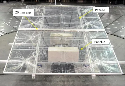
(lower and upper surfaces) during the tests. The total dimension of the model is 1960

mm×1990 mm with 12 mm gap between two layers which are placed in an aluminum

frames and 20 mm gap between panel 1 and panel 2. This double layer panel is assembled

on supporting structure of the actual solar panel at 25o inclination. Figure 2.6 demonstrates

(33)

Figure 2.5: Pressure test model

Pressure taps are connected to the pressure data acquisition system through vinyl tubes.

The tubes connectivity are described in detail in Section 2.6. Four circular holes with 50

mm diameter are provided on the lower surface of each panel as a way out for the tubes

from the layers. The pressure taps layout on upper and lower sheets are displayed in Figure

2.7a and 2.7b.

The second test model is a full-scale solar panel fabricated with the same material and

elements of a real solar panel (Figure 2.8), hence representing a full aero elastic model.

This model consists of two individual panels placed at the top and bottom of the assembly

with the same dimensions of the first model.

The inclination of the solar panels is set at 25° as typically used for southern Ontario

latitude, for high energy product during summer seasons. Both models are mounted on

three force balances in order to monitor their support reactions under a real wind loading

profile. However, the real model is specifically employed to measure their support Panel-1

(34)

reactions during the wind testing. The support reactions of the real models are recorded,

for further structural analysis.

Figure 2.6: Pressure test model set-up in WindEEE

The wind pressure measurements are further used for Finite Element analysis conducted

on supporting structure and the force-balance measurement is used to validate the FE

(35)

(a)

(b)

Figure 2.7: Tap layout of a panel (a) upper surface (b) lower surface (127 pressure

(36)

Figure 2.8: Aero-elastic model (full-scale solar panel) test set-up at WindEEE

2.4 Supporting structure of solar panel

The supporting structure of solar panel (solar Rack) is consisted of cold-form aluminum

uni-strut sections which are bolted together with proprietary connections. The solar panel

is placed in an aluminum frame which is clipped to the solar rack. Ground-mounted solar

panels are usually connected together in a network consists of several rows and columns.

The network of solar panels are usually stabilized using concrete ballast which adds to the

weight of solar network and lead to higher stability. In a real network, two ballasts on each

solar rack is placed. The same arrangement for a stand-alone solar panel using two concrete

ballasts is used in th

e

present study. The plan and elevation view of the solar rack as well

the location of concrete ballast are shown in Figure 2.9. It is worth mentioning that the

stability of a single solar panel is not the objective of this experimental work, as the stability

(37)

Figure 2.9: Solar panel supporting structure, concrete ballasts and location of force

balances

2.5 Test arrangement in WindEEE

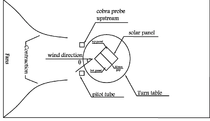
The schematic view of the entire plan of the test assembly is demonstrated in Figure 2.10.

As shown in the figure, the model is placed on the turntable at the middle of the test

chamber of WindEEE which could be adjusted for different wind angles of attack. A

contraction with an area ratio of 36% is used to produce higher flow uniformity and to

(38)

Figure 2.10: Schematic view of test setup in WindEEE

A pitot tube and a Cobra probe are utilized to measure the real-time velocity and pressure

as shown in Figure 2.11. Pitot tube is typically used for wind experiments to measure the

flow speed using differential pressure. Pitot tube is a slender tube with two holes; the front

hole measures the total pressure and the side hole measures the static pressure. Using the

difference between these pressures which is the dynamic pressure, pitot tubes calculates

the flow velocity. Cobra Probe is a multi-hole pressure probe which is used to measure the

velocity and local static pressure in real time. Cobra Probe operates in high frequencies and

(39)

Figure 2.11: Cobra Probe and Pitot tube set-up in WindEEE

2.6 Instrumentation

The pressure taps of the solar panel model are connected to the data acquisition system

through vinyl tubes with 1 mm diameter and 508 mm length. The tubes are clustered and

pass through the holes of lower sheets. The other free side of the tube is attached to another

tube with the same length and diameter through a brass restrictor in order to add more

damping and reduce the response harmonics in the pressure instrumentation system (Figure

2.12). The tubes are ultimately connected to the scanners, as shown in Figure 2.13. For this

study 16 scanners are required, each connected to 32 pressure taps (total number of 508

pressure taps) and the rest four ports of the scanners are connected to Pitot-tubes and cobra

probe to measure the reference velocity. An attempt is made to attach all the tubes and the

rack members to minimize their effect on the wind flow on the lower sheets during the

experimentation.

Cobra probe

(40)

Figure 2.12: View of the connection of vinyl tubes using brass connectors

Figure 2.13: Bottom view of solar model showing the vinyl tubes and scanners

The scanners read the pressure time series at each tap, convert them to an electrical signal

and transmit the signals to the WindEEE’s computerized data acquisition (DAQ) system. Scanner

(41)

Each of the 16 scanners is connected to the DAQ (two Inithium M921001 (283) &

M921002 (284)).The unit of recorded pressure data is an inch of water. The data is then

converted to Pascal and transformed to pressure coefficients (Cp). The instrumentation and

connection of the test set-up in the WindEEE is displayed in Figure 2.14.

Three force balances are installed under the solar racks to measure the wind induced base

reactions. These instruments are connected to three different linear power supply box

which are connected to JR3 (analog signal output). Then, the data are converted to NIDS

(National Instruments Data acquisition System) through black DC (direct current) cables

(Figure 2.14.). These force balances are capable measuring six components at the base of

the racks: three force components in X, Y, and Z directions and three moment components

about the X, Y, Z axes. It is initially clear that since the solar racks are truss-like frames

and their supports are not rigid, the moment reactions are not considerable. The obtained

forces and moments represent the overall loads transferred from the solar panels and its

framing as well as the ballast. Throughout this study, however, the wind induced reactions

are initially distinguished from the weight induced reactions for the sake of comparison of

results.

(42)

2.7 Test procedure

The model is placed on a turntable and is connected to the WindEEE pressure DAQ system

as described earlier. The solar panel model is subjected to uniform and boundary layer flow

for open exposures and pressure data are recorded as summarized in Table 2.1. The real

solar panel is tested for the same flows however, only their base reactions are recorded.

Table 2.1: The experimental test cases in WindEEE

Flow panels Angle of attack (θ)

Boundary layer

flow Aero-elastic model

0 o_{, 10} o_{, 20} o_{, 30} o_{, 40} o_{, 45} o_{, 50} o_{, 60} o_{, 70} o_{, 80} o_{, 90} o_{, 100} o_,

110 o_{, 120} o_{, 130} o_,135 o_{, 140} o_{, 150} o_{, 160} o_{, 170} o_{, 180} o

Boundary layer flow

Aerodynamic model

0 o_{, 10} o_{, 20} o_{, 30} o_{, 40} o_{, 45} o_{, 50} o_{, 60} o_{, 70} o_{, 80} o_{, 90} o_{, 100} o_,

110 o_{, 120} o_{, 130} o_,135 o_{, 140} o_{, 150} o_{, 160} o_{, 170} o_{, 180} o

Uniform flow Aerodynamic

model 0

o_{, 30}o_{, 45}o_{, 135}o_{, 150}o_{and 180}o

The duration of each test and data recording is three minutes, which is statistically-long

enough to obtain an accurate mean pressure. The pressure is measured at the frequency

value of 600 Hz. The tests are carried out for 21 wind angles at 10-degree intervals from

0o to180o in addition to 45o and 135o. However, the results from many of the oblique wind

angles (e.g. 10, 20, 30, and 40 and corresponding angles in other quarters) are not discussed

in detail in this study, as they are found to be non-critical.

The blockage ratio recorded at the WindEEE was 3%, which is less than the minimum

value recommended in ASCE-7 equal to 8% [ASCE 2010]. Table 2.2 summarizes some

characteristic of the pressure test.

Pressures are measured with respect to the mean static pressure at the WindEEE test

section, corresponding to the mean static pressure in the full-scale wind flow. At the

location of each pressure tap, the time history of the pressure coefficient, Cp(t), is obtained

from the time history of the instantaneous surface pressure, p(t), as follows:

Cp(t) =p(t) − p₁ static(t)

2ρU2

(43)

where ρ is the air density at the time of the test, and U is the mean wind speed measured at

the mean height of the solar panel over the entire test duration.

Table 2.2: Characteristic of the pressure test

Scale Blockage at WindEEE

[%] Record length of each test [s] Sampling rate [Hz]

full-scale 3% 180 600

The net pressure on each tap is evaluated through the difference between pressures on the

two corresponding taps on both sides of the solar panel. The net pressure coefficient at

each tap, Cpnet(t), is the simultaneous difference between the pressure coefficient at the

upper surface, Cpupper(t), and the corresponding pressure coefficient at the lower surface,

Cplower(t), at the same location (Equation 2.2).

Cpnet(t)= Cpupper(t)- Cplower(t) (2.2)

The obtained results of pressure tap and force balances are discussed and analyzed in detail

(44)

Chapter 3

3

Aerodynamic data analysis and discussion

This chapter outlines the results and discussion of the wind testing conducted on solar panel

models. The pressure contours for different wind profiles and various wind angles of attack

are presented. The accuracy of different pressure tap layouts and resolutions are

investigated and the Reynolds number for the wind profile is discussed. The base reactions

that calculated from the force balances are compared with those obtained from the pressure

taps. Finally, critical wind directions are recognized and several conclusions are made.

Results of comparative analyses with other studies are discussed and conclusions are

summarized.

3.1 Surface pressure distribution

The mean and net pressure coefficient contour plots for upper and lower panels are

displayed in Figure 3.1 for four wind angles of attack of 0o, 45o, 135o and 180o. The results

are obtained for boundary layer wind profile with 50% of the fan speed (mean reference

velocity of 56.2 km/h) and a roughness value of 0.01. The results for the critical wind

angles of attack are presented in the following sections.

3.1.1 Head on, forward wind angle of attack (0

o

)

The pressure distribution on the model at 0o_{wind angle of attack is almost symmetric about}

the center line of the panel. The contour plot also reveals that the positive magnitude of the

pressure coefficients is largest at the leading edge where the flow first impacts the model.

As the flow passes over the panel towards the trailing edge the pressure drops. Shademan

et al. (2010) previously identified the same pressure distribution and critical locations at 0o

wind angle of attack for a similar inclination of solar panel in a CFD simulation. There is

a little variation between the two panels as a result of the gap presence. The 20 mm gap

between the panels induces an abrupt change in pressure distribution in the direction of the

(45)

Wind

AOA Net mean Cp Upper surface Cp mean Lower surface Cp mean

0 degree

45

degree

135

degree

180

degree

Figure 3.1: Mean and net pressure coefficient (Cp) contours on the panels for

(46)

3.1.2 Head on, reverse wind angle of attack (180

o

)

The contour plots of net pressure coefficient show that the panel is critically loaded when

the wind angle of attack is head-on at 180o _{wind angle of attack. When the flow approaches}

the solar panel in the reverse direction, i.e. 180o wind angle of attack, the lower surface

faces the approaching wind while the upper surface lies in the wake of the wind flow. The

pressure distribution on the lower surface, which now faces the oncoming wind, is also

symmetric across the mid plane. As the upper surface pressure is subtracted from lower

surface pressure, the mean net pressure is a negative value across two panels as shown in

Figure 3.1.

3.1.3 Oblique wind angles of attack (45

o

_{and 135}

o

₎

When the wind approaches the model at angles other than 0o and 180o, there is no symmetry

of the pressure distribution across the panel, as displayed in contour plot of Figure 3.1. The

asymmetric pressure distribution pattern is also obtained for other oblique angles from 10o

to 170o. Figure 3.1 demonstrate that mean Cp values decrease diagonally on the surfaces

of panels along the wind angle of attack. This is expected as the flow accelerates at the

leading edges or corners and creates a low pressure region on the panel surface and

gradually decrease in the flow direction, forming a horseshoe vortex.

Mean Cp distributions of oblique angles illustrate a separated region for both 45o_{and 135}o

wind angles of attack which confirms possible existence of corner vortices. Formation of

the separated region and corner vortices are more pronounced on panel-1 (top panel) while

a mean Cp of the panel-2 show almost a modest uniform distribution. For 45o_{and 135}o

wind angles of attack, the asymmetric pressure distribution and corner vortices are also

(47)

3.2 Pressure equivalent

For the design and stability control of the solar racks, the total wind force on the panels is

required, which is obtained by integrating the pressure on the panel surface with the

corresponding tributary area. This pressure integration is given by Equation 3.1 which is

the summation of pressure multiplied by its tributary area at each tap.

𝐹_𝑡 = ∑ 𝑝_{𝑛𝑒𝑡,𝑖} 𝑛

𝑖=1

× 𝐴_𝑖

(3.1)

where Ft is total force applied on panel, pnet,i represents the net pressure on tributary area

of the tap number “i”, and Ai is the tributary area of the tap number “i”.

The equivalent pressure (Peq) is evaluated as the total force divided by the total area of the

panels using Equation 3.2. The physical meaning of Peq is that if a uniform pressure with

the value of Peq is applied on the surface of a solar panel, it creates the same magnitude of

force as the original pressure. By implementing Peq, the variation of the applied load on the

panels can be easily illustrated in different wind angles of attack as shown in Figure A.1 in

appendix A. Which Peq is usually expressed in terms of a dimensionless wind pressure

parameter that is referred as equivalent pressure coefficient (CPeq.) and is defined as

Equation 3.3.

𝑃_𝑒𝑞= ∑ 𝑝𝑛𝑒𝑡,𝑖 𝑛

𝑖=1 × 𝐴𝑖

∑𝑛_𝑖=1𝐴_𝑖 (3.2)

𝐶𝑝_𝑒𝑞 =∑ 𝐶𝑝𝑛𝑒𝑡,𝑖 𝑛

𝑖=1 × 𝐴𝑖

∑𝑛 𝐴_𝑖

𝑖=1 (3.3)

where Vo is reference velocity equal to 15.88 m/s. Figure 3.2a, 3.2b and 3.2c represent

mean, maximum and the minimum equivalent pressure coefficient on panels, respectively,

obtained from the time history of the pressure taps. The maximum and minimum values

are obtained statistically by using the method of Gumbel distribution assuming the

probability of non-exceedance of 95%. Figure 3.2a shows that the maximum force occurs

between 160o and 180o wind angle of attack, while Figure 3.2c confirms that the maximum

force occurs at 180o wind angle of attack. So the stability of the solar panel should be

controlled in the most critical direction which is the transverse drag force (180o). Figure

(48)

Figure 3.2: (a) Mean, (b) maximum and (c) minimum equivalent pressure coefficient

for all wind angles of attack

3.3 Pressure coefficient comparison with literature

The pressure coefficients on the full-scale solar panel model of the present study are

compared with the results of the 1:10 scaled experiment conducted by Aly and Bitsuamlak

(2013) in the Boundary Layer Wind Tunnel Laboratory. This comparison is carried out for

similar inclination angle of the panel (25o) and wind angle of attack of 0o and illustrated in

Figure 3.3. It is to be noted that the solar panel tested by Aly and Bitsuamlak (2013) is

longer 9200 mm×1400 mm compared to the present solar panel which is 1960 mm×1990

mm. Figure 3.3 shows that the pattern of the net pressure coefficient of the scaled solar

panel model is in agreement with the full scale solar panel model obtained in this study. -0.90 -0.60 -0.30 0.00 0.30 0.60

0 30 60 90 120 150 180

equi val ent pre ss ure coe ffic ie nt (m ea n)

Wind angle of flow Mean Cpeq. Cpequivalent_mean 0.00 0.50 1.00 1.50 2.00

0 30 60 90 120 150 180

equi val ent pre ss ure coe ffic ie nt (m ax)

Wind angle of flow Max Cpeq. Cpequivalent_max -3.20 -2.80 -2.40 -2.00 -1.60 -1.20 -0.80 -0.40 0.00

0 30 60 90 120 150 180

equi val ent pre ss ure coe ffic ie nt (m in)

Wind angle of flow Min Cpeq.

Cpequivalent_mean (a)

(49)

Figure 3.3: Comparison of mean net pressure coefficient of solar panel with 25o

slope, a) 1:10 scale (Aly et al. 2012), b) full-scale model

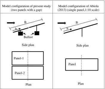
Another comparison analysis is carried out with the aerodynamic results presented in

Abiola-Ogedengbe et al. (2015). Figure 3.4 shows the model configuration for the two

studies. Abiola-Ogedengbe et al. (2015) investigated an experimental model of a single

panel at 1:10 scale (with 25o inclination) in the Wind Tunnel I at the University of Western

Ontario. Figures 3.5 and 3.6 compare the mean Cp values along the mid-line of the panel

for 0o and 180o wind angles of attack in both studies, respectively. To make the comparison

meaningful, reference pressure and wind speed for calculation of Cp are taken at the same

location. For the sake of comparison, the results are also normalized to the unit width of

the panel to avoid the effect of different geometries.

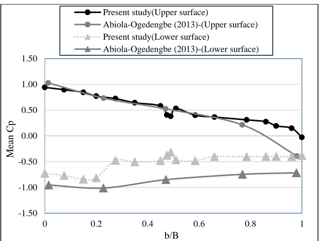
A fairly good match is observed between Cp of the upper panel of both studies in 0o and

180o_{, however, there is an abrupt change in the present study graphs at the middle of flow}

path (50% b/B) which can be attributed to the presence of 20 mm gap between panel-1 and

panel-2.

The graphs of the mid-line Cp of the lower surface of the panels are not in an agreement as

good as the upper surface. This difference in pressure on the lower surface of the solar

panel is attributed to the presence of the large concrete ballasts in the full-scale assembly

which will alter flow condition on the lower surface of the solar panel. This can be clearly

(50)

seen in graphs of Figure 3.6 where b/B=1. The pressure tubes coming out from the lower

surface of the solar panel may have contributed, but it is very significant compared to the

concrete ballast. The 1:10 scaled model of Abiola-Ogedengbe et al. (2015) pulled the

pressure tubes from side edges which created good condition for 00_{and 180}0_{wind angle}

of attack. However, this arrangement cannot be used for the oblique wind angles of attack.

Despite the justifiable differences in the lower surface of solar panels and that of the effect

of the gap, the magnitude and the variations of the Cps over the solar panels show good

agreement between the two studies carried out at different scales. This confirms the

conclusion made by Aly and Bitsuamlak (2014) stating that within the geometric scale of

1:10 to 1:50, mean wind loads on the solar panels are independent of the model scale (Aly

and Bitsuamlak 2013).

Model configuration of present study (two panels with a gap)

Model configuration of Abiola (2013) (single panel,1:10 scale)

Figure 3.4: Model configuration of present study and Abiola-Ogedengbe (2013)

with 25o_{inclined panel at 0}o_{wind angle of attack}

b

Plan B

Panel

Side plan B

Ballast b

Side plan

Panel-1

Panel-2

(51)

Figure 3.5: Mean Cp profiles along the mid-line of the panel surface for wind angles

of attack of 0o

Figure 3.6: Mean Cp profiles along the mid-line of the panel surface for wind angles

of attack of 180o_Figure

-1.50 -1.00 -0.50 0.00 0.50 1.00 1.50

0 0.2 0.4 0.6 0.8 1

Me

an C

p

b/B

Present study(Upper surface)

Abiola-Ogedengbe (2013)-(Upper surface) Present study(Lower surface)

Abiola-Ogedengbe (2013)-(Lower surface)

-2.00 -1.50 -1.00 -0.50 0.00 0.50 1.00 1.50

0 0.2 0.4 0.6 0.8 1

Me

an C

p

b/B

Present study-middle-(Upper surface)

Abiola-Ogedengbe (2013)-(Upper surface)

Present study-middle-(Lower surface)

(52)

3.4 Effect of pressure tap resolutions

One of the common challenge, while testing small structures (such as solar panel, roof

pavers etc.) in the traditional boundary layer wind tunnel is their small size, limiting the

number of taps that can be installed (Aly and Bitsuamlak 2013, Aly and Bitsuamlak 2012,

Asghary et al. 2014) . The present study, owing to its large size, allows to study the effect

of tap resolution on the overall wind loading and the ability to capture local pressure

distribution. In the present study, wind pressure on the solar panel model is measured

through 254 pressure taps incorporated in each of lower and upper sheet of the panel (total

number of taps 508). The number of the taps divided by the area of the panel can describe

the tap resolution. Incorporating higher density of pressure taps (hence higher resolution)

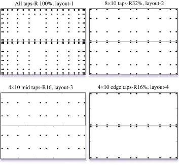
clearly helps to accurately measure the pressure distribution.

A comparative study is carried out to evaluate the effect of arrangement and resolution of

the pressure taps. Figure 3.7 shows the four resolutions that are considered in the present

comparison. The 508 tap usage is referred as R100 to represent Resolution of 100% taps

used (i.e. high resolution). Some of the taps are eliminated from the analysis to create less

resolution tap layouts. Accordingly, the following tap resolutions are created: R32%,

R16% with mid taps (layout-3) and R16% with edge taps (layout-4) as shown in Figure

3.7. The full tap layout (R 100%) is selected as a benchmark to evaluate the low resolution

tap layouts which are in fact comparable to those used in the traditional boundary layer

(53)

Figure 3.7: Pressure tap layout for four different resolutions

The mean net pressure coefficient contours for each tap resolution are plotted for 0, 45,

135 and 180 degree wind angles of attack as shown in Figures 3.8, 3.10, 3.12 and 3.14,

respectively. The equivalent minimum, maximum and mean net pressure coefficients

(Cpmin, Cpmax and Cpmean) are also evaluated for each case and plotted in Figures 3.9, 3.11,

3.13 and 3.15. The peak and mean equivalent net pressure coefficients (Cpmin, Cpmax and

Cpmean) are evaluated following a similar procedure discussed for equivalent pressure (see

Equation 3.2).

The following observations are made from comparisons shown in Figures 3.8 to 3.15:

 It appears that a high density resolution is required to capture all the aerodynamic

features of pressure on the solar panel surfaces. However, layout-2 (R32%) in all

cases, fairly represents the pressure distribution without compromising the

4×10 mid taps-R16, layout-3

8×10 taps-R32%, layout-2 All taps-R 100%, layout-1

Wind Loading on Full-scale Solar Panels

Scholarship@Western

Scholarship@Western

Wind Loading on Full-scale Solar Panels

Wind Loading on Full-scale Solar Panels

Keywords

Co-Authorship Statement

Acknowledgments

Table of Contents

List of Tables

List of Figures

List of Appendices

Nomenclature

Chapter 1

1

Introduction

1.1

WindEEE Dome

1.2

Wind pressure measurements

1.3

Literature review

1.4

Motivations

1.5

Objectives

1.6

Organization of the thesis

Chapter 2

2

Test set-up and methodology

2.1

Background

2.2

Boundary layer development at WindEEE

2.3

Experimental models

2.4

Supporting structure of solar panel

e

2.5

Test arrangement in WindEEE

2.6

Instrumentation

2.7

Test procedure

Chapter 3

3

Aerodynamic data analysis and discussion

3.1

Surface pressure distribution

3.1.1 Head on, forward wind angle of attack (0

)

3.1.2 Head on, reverse wind angle of attack (180

)

3.1.3 Oblique wind angles of attack (45

and 135

)

3.2

Pressure equivalent

3.3

Pressure coefficient comparison with literature

3.4

Effect of pressure tap resolutions

_{and 135}

₎