PERFORMANCE ANALYSIS OF OS STRUCTURE OF CFAR DETECTORS IN FLUCTUATING TARGET ENVIRONMENTS
M. B. El Mashade
Electrical Engineering Dept., Faculty of Engineering Al Azhar University
Nasr City, Cairo, Egypt
Abstract—This paper is intended to the analysis of adaptive radar
pulse. Under the multiple-target operations, the ML-OS detector has the best homogeneous performance, the MN processor has the best multitarget performance when a cluster of radar targets appears in the reference window, while the MX scheme doesn’t offer any excessive merits, neither in the absence nor in the presence of outlying targets, as expected.
1. INTRODUCTION
under conditions in which the signal and noise statistics are known. Nonlinear receivers attempt to control the processor gain as a function of the interference level to provide the desired CFAR action. In general, nonlinear receivers exhibit a large CFAR loss.
The most conventional CFAR schemes are of the mean-level type such as the cell-averaging (CA) and its modified versions [1– 3, 7, 15, 16]. The CA-CFAR detector uses the maximum likelihood estimate of the noise power to set the threshold adaptively on the assumption that the underlying noise distribution is exponential and the noise samples are independent and identically distributed (IID). Unfortunately, its detection performance degrades considerably in nonhomogeneous situations caused by multiple targets and clutter edges. The CA processor turns out to performvery poorly in these situations, and if some resilience against interferers and/or clutter edges is to be gained, alternative schemes, must be adopted.
Greater robustness has been obtained with the data censoring algorithms. These systems rely on ordering or ranking the samples in the reference window and take an appropriate reference cell to estimate the background clutter power level. This allows censoring of a certain number of outliers, and consequently the censoring schemes perform creditably as long as the number of interfering targets does not exceed the number of top ranked censored samples. The ordered-statistic (OS) detector has small additional detection loss over the CA-CFAR detector in uniformnoise background and can resolve closely spaced targets [5, 7]. However, the large processing time required by this technique limits its practical use. To reduce this processing time in half, the modified versions of this processor have been suggested. They have been proposed by Elias-Fuste [8], and analyzed by You [10], and El Mashade [11] for their performance evaluation in the single sweep case. Noncoherent integration analysis of these processors is carried out in [9] for their performance evaluation in homogeneous background, and their nonhomogeneous performance has been analyzed by El Mashade [14]. Finally, El Mashade [13] analyzed their M-correlated sweeps in nonhomogeneous situations.
SWII & SWI models). The detection of this type of fluctuating targets is of great importance. In order that our previous work [14] be sufficiently general to be applicable to a variety of cases, our goal in the present paper is to analyze the performance of the OS based detectors for partially correlated χ2 targets with two degrees of freedomin the absence as well as in the presence of spurious targets. The χ2 target model includes the well known SWI and SWII models as special cases. In section II, we formulate the problem and compute the moment generating function of the postdetection integrator output for the case where the signal fluctuation obeys χ2 statistics with two degrees
of freedomthat is considered for the study of the signal processing algorithms. The performance of the schemes under consideration is analyzed in Section 3 and their performance is assessed in Section 4. In Section 5, we present a brief discussion along with our conclusions.
2. BACKGROUND AND PROBLEM FORMULATION
3 3
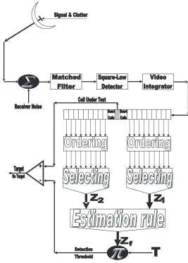
Figure 1. Architecture of OS structure of CFAR detectors with
postdetection integration.
to estimate the unknown noise power level. In this manuscript, we are concerned with the CFAR processors in which the ordered-statistic (OS) technique is implemented. The detection problem consists of testing the hypothesisH0 (absence of signal) versus the alternativeH1
(presence of signal). Precisely, we have
y(t) =
n(t) under H0
s(t) +n(t) under H1
[0, T0] represents the observation interval, s(t) and n(t) denote the
baseband equivalents of received waveformand noise, respectively. In order to analyze the detection performance of a CFAR processor, let the input to the square-law detector consists ofM pulses, each composed of a steady signal component and Gaussian noise. Denote the in phase and quadrature components of the signal over theM pulses by theM×1 vectorsSi andSq, respectively, and denote the in phase and quadrature components of the noise byM×1 vectors
NiandNq, respectively. Then, the integrated output of the square-law detector is
Y ∆− |Si+Ni|2+|Sq+Nq|2 (2) The moment generating function (MGF) associated with the random variable (RV)Y is defined as
MY(ω) ∆−
∞
−∞
fY(x) exp(−ωx) dx (3)
In the above expression,fY(.) denotes the probability density function (PDF) of Y. Substituting Eq. (2) for the randomvariable Y, Eq. (3) takes the form
MY(ω) =
∞
−∞ ∞
−∞
f(Ni, Nq) exp
−ω|Si+Ni|2+|Sq+Nq|2
dNidNq (4) IfNi and Nq are Gaussian and IID randomvectors, one may write
f(Ni, Nq) =
1 2πσ2
M
exp
−|Ni|2+|Nq|2
2σ2 (5)
The substitution of Eq. (5) into Eq. (4) yields
MY(ω) =
1 2πσ2
M ∞
−∞ ∞
−∞
exp
−|Ni|2+ 2ωσ2|Si+Ni|2 2σ2
×exp
−|Nq|2+ 2ωσ2|Sq+Nq|2
2σ2 dNidNq (6)
Completing the squares inNi andNq and integrating overNi and Nq, one obtains
MY(ω) =
1 1 + 2ωσ2
M
exp
−ω
|Si|2+|Sq|2
If the signal component fluctuates, then the MGF of the square-law detector is a weighted average, accounting for the PDF of the in phase and quadrature components of the signal. Hence, for a fluctuating target, the MGF of the detector output is [6]
MY(ω) =
∞
−∞ ∞
−∞
MY(ω)fSi(Si)fSq(Sq) dSidSq (8)
Assuming that Si and Sq are IID with PDF S(x), we have
MY(ω) =
1
1 + 2ωσ2 M
∞
−∞
fS(X) exp
− ω|X|2
1 + 2ωσ2 dX 2
(9)
Using Eq. (9), one may compute the MGF for any target PDF.
2.1. Correlated χ2 Signal Model
Most radar targets are complex objects and produce a wide variety of reflections. Different targets often require different models to characterize the varied statistical nature of these responses. A radar target whose return varies up and down in amplitude as a function of time is known as fluctuating target. The fluctuation rate may vary fromessentially independent return amplitudes frompulse-to-pulse to significant variation only on a scan-to-scan basis. Theχ2 family is one of the most radar cross-section fluctuation models. Theχ2 distribution with 2K degrees of freedomhas a PDF given by
fS(σ) = 1 Γ(K)
K σ
K
σK−1exp
−K σσ
U(σ) (10)
In the above expression, σ is the average cross section over all target fluctuations and U(.) denotes the unit step function. When K = 1, the PDF of Eq. (10) reduces to the exponential or Rayleigh power distribution that applies to the Swerling cases I and II.
The above formula represents the PDF of the sum of the squares of 2K real Gaussian RV’s or the sumof the squared magnitudes ofK
complex Gaussian RV’s. Therefore, ifK = 1, thenσmay be generated asσ =x21+x22, where xi, i= 1,2, are IID Gaussian RV’s, each with zero mean andσ/2 variance. The magnitude of the in phase component isu=x1. Ifα=σ/2, we can write the PDF ofu as
fu(x1) =
1
√
2παexp
−x21
To accommodate an M ×1 vector of correlated χ2 RV’s with two degrees of freedom, we introduce the PDF of theM-dimensional vector
X1
fX1(X) =
1 2πα M 2 1
|Λ|exp
−XTΛ−1X
2α (12)
In the above expression, Λ represents the correlation matrix of
x11, x12, . . . , x1M andT denotes the vector transpose. The substitution of Eq. (12) into Eq. (9) yields
MY(ω) =
1 1 + 2ωσ2
M ∞ −∞ 1 2πα M 2 1
|Λ|exp
− 1
2αX
T
Λ−1+ 2ωα 1 + 2ωσ2I
X dX 2 (13)
I denotes the identity matrix. Carrying the above integration leads to
MY(ω) =
1
|(1 + 2ωσ2)I+ 2ωαΛ| (14)
Expressing the determinant in terms of the nonnegative eigenvalues
λ1, λ2, . . . , λM of Λ, Eq. (14) takes the form
MY(ω) = M
i=1
1 1 + 2ω(σ2+αλ
i) = M i=1 1
1 +ψ(1 +Aλi)ω
(15)
ψ = 2σ2 represents the noise power and A = 2α/ψ is the average signal-to-noise ratio (SNR). It is important to note that MY(ω) is the Laplace transformation of the PDF of the sum of M square-law detected pulses of aχ2 (K = 1) signal in Gaussian noise.
The Swerling case I (slow fluctuation) model is represented by choosingλ1 =M, λi= 0 for 2≤i≤M. Thus, for SWI, we have
MY(ω) =
1
1 +ψ(1 +M A)ω
1 1 +ψω
M−1
for SWI model (16)
which agrees with Swerling’s result [12]. The fast fluctuation (SWII), on the other hand, can be represented by choosingλi = 1 for 1≤i≤
M, which yields
MY(ω) =
1 1 +ψ(1 +A)ω
M
In view of Eq. (15), the solution for the partially correlated case requires computation of the eigenvalues of the correlation matrix Λ. It is assumed here that: i) The statistics of the signal are stationary, and ii) The signal can be represented by a first order Markov process. Under these assumptions, Λ is a Toeplitz nonnegative definite matrix of the following general form:
Λ =
1 ρ ρ2 · · · ρM−2 ρM−1
ρ 1 ρ · · · ρM−3 ρM−2 ρ2 ρ 1 · · · ρM−4 ρM−3
· · · · · · · ·
· · · · · · · ·
· · · · · · · ·
ρM−2 ρM−3 ρM−4 · · · 1 ρ ρM−1 ρM−2 ρM−3 · · · ρ 1
0≤ρ≤1
(18) Eqs. (15)–(18) are the basic formulas of our analysis in this paper.
The PDF of the output of theith test tap is given by the Laplace inverse of Eq. (15) after making some minor modifications. If theith test tap contains noise alone, we let A = 0, that is the average noise power at the receiver input isψ. If theith range cell contains a return from the primary target, it rests as it is without any modifications, where A represents the strength of the target return at the receiver input. On the other hand, if theith test observation is corrupted by interfering target return, A must be replaced by I, where I denotes the interference-to-noise (INR) at the receiver input.
3. PROCESSOR PERFORMANCE EVALUATION IN MULTITARGET SITUATIONS
describe transition areas between regions with very different noise characteristics. Multiple target situations occur occasionally in radar signal processing when two or more targets are at a very similar range. The consequent masking of one target by the others is called suppression. These interferers can arise fromeither real object returns or pulsed noise jamming. From a statistical point of view, this implies that the reference samples, although still independent of one another, are no longer identically distributed. In our analysis and study of the nonhomogeneous background for which the reference cells don’t follow a single common PDF, we are concerned only with increases in the value of ψ for some isolated reference cells due to the presence of secondary targets. The amplitudes of all the targets present amongst the candidates of the reference window are assumed to be of the same strength and to fluctuate in accordance with the partially correlatedχ2
fluctuation model with correlation coefficient ρi. The interference-to-noise ratio (INR) for each of the spurious targets is taken as a common parameter and is denoted by I. Thus, for reference cells containing extraneous target returns, the total background noise power isψ(1+I), while the remaining reference cells have identical noise power of ψ
value.
The ordered-statistic (OS) CFAR detector uses the Kth smallest sample to estimate the total noise power. We will denote by OS(K) the OS scheme with parameter K. The value of K is generally chosen so that the detection probability (in homogeneous background) is maximized. The large processing time taken by this detector in ordering the candidates of the reference window limits its practical uses. Modified versions of this processor have been proposed to solve this problem[8]. Such detectors are specifically tailored to provide good estimates of the noise power as the conventional OS detector. In this section, we analyze the conventional OS scheme as well as three of its modified versions, namely ML-, MX-, and MN-OS schemes, for their performance evaluation in multitarget environment and obtain closed formexpression for their detection performances.
3.1. Single-Window OS Detector
The amplitude values taken from the reference window, of size N, are first rank-ordered according to increasing magnitude. The sequence thus achieved is
q(1)≤q(2)≤q(3)≤. . .≤q(K) ≤. . .≤q(N) (19)
The indices in parentheses indicate the rank-order number. q(1)denotes
Eq. (19) is called an ordered-statistic. The central idea of an ordered statistic CFAR processor is to select one certain value fromthe above sequence and to use it as an estimate Z for the average clutter power as observed in the reference window. Thus,
ZOS =q(K), K∈ {1,2,3, . . . , N} (20)
In the CFAR system, target decision is commonly performed by multiplying this estimation ZOS by a scaling factor T, which is dependent on the applied estimation technique and the required rate of false alarm. The resulting product ZOST is directly used as the threshold value with which the content of the cell under test Y is compared to decide whether the target is present or absent. A target is declared to be present ifY exceeds the thresholdT ZOS. The threshold coefficient T is used to achieve a desired false alarmrate for a given window sizeN when the total background noise is homogeneous. Since the unknown noise power level estimate Z is a randomvariable, the processor performance is determined by calculating the average values of false alarmand detection probabilities. The false alarmprobability
Pf a is defined as
Pf a ∆−Ez{P(YZT|H0)}= 1−Ez{FY(ZT)} (21) In the above expression, EZ(.) denotes the expectation operator and
FY(.) represents the cumulative distribution function (CDF) of the randomvariable Y. When the background clutter is homogeneous,Y
has a MGF given by Eq. (15) after settingA equals to zero.
MY(ω) =
1 1 +ψω
M
(22)
The Laplace inverse of Eq. (22) gives the PDF of Y under the null hypothesis (H0). Thus,
fY(y|H0) =
1
ψ
M 1
Γ(M)y
M−1exp
−y ψ
U(y) (23)
Once the PDF of Y is obtained, we can calculate its associated CDF, which is in turn used to compute the probability of false alarm. Finally,
Pf a takes the form
Pf a= M−1
j=0
T ψ
j (−1)j Γ(j+ 1)
dj
In the above formula, MZ(.) denotes the MGF of the noise level estimate Z. For a CFAR scheme, MZ(T /ψ) must be independent of
ψ. This is indeed true for all the detection schemes considered here. Under the signal present hypothesis H1, the statistic Y has a MGF
given by Eq. (15) which can be put in another simplified form
MY(ω) = M
j=1
aj
ω+aj
with aj −Λ
1
ψ(1 +Aλj)
(25)
By using the technique of partial fraction method, the PDF of the cell under test variateY becomes
fY(y|H1) =
M
i=1
Diexp(−aiy)U(y) (26)
The constantsDi’s are defined as
Di ∆=ai M
j=1
j=1
aj
aj−ai
(27)
Once the PDF of the cell under test variate Y is calculated, the execution of its associated CDF is straightforward. Finally, the processor detection performance takes the following analytical form
Pd= M
i=1
Di
ai {
Mz(ω)}ω= T ψ(1+Aλi)
(28)
In order to analyze the processor performance when the reference window no longer contains radar returns froma homogeneous background, the assumption of statistical independence of the reference cells is retained. Consider the situation where the reference window contains r interfering target returns, each with power level ψ(1 +I), and the remainingN−rsamples having thermal noise only with power level ψ. Under these assumptions, the Kth ordered sample, which represents the noise power level estimate in the OS detector, has a CDF given by [14]
FK(z;N, r) = N
i=K
min(i,N−r)
j=max(0,i−r)
N−r j
r i−j
The CDF of the reference cell that contains a spurious target return can be obtained from
Fs(z) =L−1
1 ω M =1 1
1 +ψ(1 +Iλ)ω
= 1− M
=1
be−cz (30)
whereL−1 denotes the Laplace inverse operator and
b ∆− M
k=1
k=
1 +Iλ
I(λ−λk)
and c ∆− 1
ψ(1 +Iλ)
(31)
Ft(.) represents the CDF of the reference cell that contains thermal noise only of background power ψ. This CDF is associated with a PDF of a similar form as that given by Eq. (23), which by integrating it we obtain the desired CDF. Thus,
Ft(z) = 1− M−1
j=0
z ψ
j 1
Γ(j+ 1)exp
−z ψ
U(z) (32)
The substitution of Eqs. (30) and (32) into Eq. (29) yields
FK(z;N, r) = N
i=K
min(i,N−r)
j=max(0,i−r)
N −r j
r i−j
×
j
k=0
i−j
=0 j k
i−j
0 (−1)
i−k−
×
M−1
m=0
z ψ
m
Γ(m+ 1)e
−z ψ
N−r−k
∗
M
n=1
bne−cnz
r− (33)
The Laplace transformation of the above equation gives
ΦFK(ω;N, r) = N
i=K
min(i,N−r)
j=max(0,i−r)
N −r j
r i−j
×
j
k=0
i−j
=0 j k
i−j
0 (−1)
i−k− N−r−k
θ0=0
· · ·
N−r−k θM−1=0
Ω(N −r−k;θ0, . . . , θM−1)
M−1
v=0
[Γ(v+ 1)]θv
1
ψ
M−1
η=0
ηθη
×
r−
ϑ1=0
r−
ϑ2=0 · · ·
r−
ϑM=0
Ω(r−0;ϑ1, . . . , ϑM) M
ξ=1
(bξ)ϑξ
×
Γ
M−1
γ=0
γθγ+ 1
ω+N −r−k
ψ +
M
ζ+1
ϑζcζ
M−1
γ=0
γθγ+1
(34)
where
Ω(N−i−1;j0, . . . , jM−1) ∆−
Γ(N−i) M−1
=0
Γ(j+ 1) for
M−1
k=0
jk=N −i−1
0 for
M−1
k=0
jk=N −i−1 (35) Once the Laplace transformation of the CDF of noise power level estimate is computed, the MGF of the final noise power level is calculated as [11]
Mz(ω) ∆=ωΦFz(ω) (36) and consequently, the processor detection performance can be easily evaluated (see Eq. (28)).
3.2. Double-Window OS Detector
Although the OS-CFAR detector has some advantages over the cell-averaging detector [7–11], the large processing time taken by this technique in sorting the reference cells limits its practical applications. To alleviate this problem, the double-windows OS procedure has been proposed [8]. Employing two simultaneously specialized processors, one for each set of neighboring cells, it is possible to reduce by half the single-window processing time without altering the estimation of the clutter statistics. On the other hand, if the leading and lagging set of cells are independently ordered and subsequently compared under the maximumor minimumcriterion, we will obtain a new randomvariable with differing statistics fromthe representative cell of the OS-CFAR algorithm.
Three modified versions of the OS-CFAR technique are analyzed in this subsection: the mean-level (ML-), the maximum (MX-) and the minimum (MN-) ordered statistic procedures. Each one of these modified versions can reduce the single-window OS processing time in half and has the same advantages as the OS detector with only a negligible increment to the CFAR loss.
In addition to aiming at reducing the number of excessive false alarms at clutter edges, the modified ordered-statistic processors may also be used in multiple target situations. Here, we examine the effects of outlying targets on detectability of the cell under test. When the number of these targets is within their allowable range, the effect of spurious targets is manifested in a change in the underlying statistical assumptions. This implies that the candidates of the reference sets, although still independent of one another, are no longer identically distributed.
3.2.1. Mean-Level (ML) OS Detector
Referring to Fig. 1, reference cells are equally partitioned into leading and lagging windows Z1 and Z2. The generic operation of the
two-windows family of CFAR detectors is to process the cells of each local window separately, and then combining the resulting estimates through a mean-level (ML) operation to obtain the final estimate of the unknown noise power level. The candidates of each local window (of size N/2) are separately ordered fromsmallest to largest and then the K1th order statistic fromthe leading subset and the K2th order
statistic fromthe trailing subset are taken to represent the unknown noise power level estimate of each local window.
Zi =q(ki), ki∈
"
1,2,3, . . . ,N
2
#
In ML-OS detector, the total noise power is estimated by combining the local noise level estimates through the mean operation. The combiner puts out the noise level estimateZM L as
ZM L =mean(Z1, Z2) (38)
The rationale for the mean family of CFAR schemes is that by choosing the mean, the optimum CFAR detector in a homogeneous background when the reference cells contain IID observations is achieved. In addition, as the size of the reference window increases, the detection probability approaches that of the optimum detector, which is based on a fixed threshold.
Since the total noise power is estimated by averaging the local estimates of the noise power levels, the MGF of ZM L is simply given by the product of the MGF’s of Z1 and Z2 [4]. Therefore,
MZM L(ω) =MZ1(ω)MZ2(ω) (39)
where
MZ1(ω) =ωΦFK1(ω;N1, r1) and MZ2(ω) =ωΦFK2(ω;N2, r2) (40) The MGF’s of the noise level estimates are given as a function of the Laplace transformation of their CDF’s. These CDF’s have the same expression as that given by Eq. (34) after replacingN andr byN1 and
r1for the statisticZ1and byN2andr2for the statisticZ2, respectively.
Here, r1 and r2 represent the number of interfering target returns
amongst the contents of the leading and trailing reference windows, respectively, and N1 = N2 = N/2. Since the MGF of the final
noise power level estimateZM L is the backbone of the processor false alarm and detection performances, the behavior of the scheme under consideration, in multiple target environments, can be easily obtained.
3.2.2. Maximum (MX)-OS Detector
overcoming only one of these problems with additional loss of detection power. The first scheme, which is known as the maximum (MX) procedure, is specifically aimed at reducing the number of excessive false alarms in the presence of abrupt change in the noise power from one level to another. The generic operation of the MX family of CFAR schemes is to process the cells from each local window separately and combining them through a maximum operation. The combiner puts out the final noise level estimate
ZM X = max(Z1, Z2) (41)
The rationale for the maximum detector is that by choosing the larger of the local noise level estimates, the increase in false alarm probability for test cells near the edges of clutter patches is avoided. In addition, when the OS technique is combined with the maximum operation, we obtain a processor that is also robust to interfering targets.
The MX-OS detector uses the maximum of the two local estimates
Z1 and Z2 to estimate the background noise power level. The CDF
associated with this noise power level estimate is [14]
FZM X(z) =FZ1(z) FZ2(z) (42)
By using the generalized formula of the CDF of the Kth ordered statistic, out of N reference samples in the presence of r interfering target returns (given by Eq. (33)), the above equation can be written as
FZM X(z) = N1
i=K1
min(i,N1−r1)
j=max(0,i−r1)
N1−r1
j
r1
i−j
×
j
k=0
i−j
=0 j k
i−j
0 (−1)
i−k−
×
M−1
m=0
z ψ
m
Γ(m+ 1)e
−z ψ
N1−r1−k
×
M
n=1
bne−cnz
r1−
FK2(z;N2, r2) (43)
By taking the Laplace transformation for the above equation, we obtain
ΦFZMX(ω) = N1
i=K1
min(i,N1−r1)
j=max(0,i−r1)
N1−r1
j
r1
×
j
k=0
i−j
=0 j k
i−j
0 (−1)
i−k−
N1−r1−k
θ0=0
N1−r1−k
θ1=0 · · ·
N1−r1−k
θM−1=0
Ω(N1−r1−k;θ0, . . . , θM−1)
M−1
v=0
[Γ(v+ 1)]θv
1
ψ
M−1
η=0
ηθη
×
r1−
ϑ1=0
r1−
ϑ2=0 · · ·
r1−
ϑM=0
Ω(r1−0;ϑ1, . . . , ϑM) M
ξ=1
(bξ)ϑξ
×(−1) M−1
γ=0
γθd M−1
γ=0
γθγ
dω M−1
γ=0
γθγ
{ΦFK2(ω;N2, r2)}
$$ $$ $
ω=ω+N1−r1−k
ψ + M
ζ=1
ϑζcζ (44)
where
(−1)m d m
dωm{ΦFK2(ω;N2, r2)}=
N2
i=K2
min(i,N2−r2)
j=max(0,i−r2)
N2−r2
j
r2
i−j
×
j
k=0
i−j
=0
j k
i−j 0
(−1)i−k−
N2−r2−k
θ0=0
N2−r2−k
θ1=0 · · ·
N2−r2−k
θM−1=0
Ω(N2−r2−k;θ0, . . . , θM−1)
M−1
v=0
[Γ(v+ 1)]θv
1
ψ
M−1
η=0
ηθη
×
r2−
ϑ1=0
r2−
ϑ2=0 · · ·
r2−
ϑM=0
Ω(r2−0;ϑ1, . . . , ϑM) M
ξ=1
(bξ)ϑξ
×
Γ
M−1
γ=0
γθγ+m+ 1
ω+N2−r2−k
ψ +
M
ζ=1
ϑζcζ
M−1
γ=0
γθγ+m+1
(45)
performance is completely determined. Consequently, the false alarm and detection probabilities of the MX-OS processor can be easily evaluated since the MGF of the noise power level estimate is the backbone of their expressions.
3.2.3. Minimum (MN)-OS Detector
The minimum operation has been introduced to alleviate the problems associated with closely spaced targets leading to two or more targets appearing in the reference window. While testing for target presence at a particular range, the processor must not be influenced by the extraneous target echoes. It has been shown that although the MN-OS detector exhibits greater additional detectability loss in homogeneous environments (relative to the other modified versions), it does perform well in multiple target environment when a cluster of radar targets appears in the reference windows.
The MN operation is capable of resolving multiple targets in the reference window as long as all the interferers appear either in the leading or lagging window. However, this scheme has undesired effects when interfering targets are located in both halves of the reference window and their number is outside their allowable range [11].
In this type of CFAR schemes, the noise power level is estimated by taking the minimum of the local noise level estimatesZ1 andZ2 as
depicted in Fig. 1. That is
ZM N = min(Z1, Z2) (46)
In this case, the noise power level estimate has a PDF given by [7]
fZM N(z) =fZ1(z) +fZ2(z)−fZM X(z) (47) The last termin the above expression is simply the PDF of ZM X for the MX-OS. All the PDF terms in the right hand side of the above expression are previously determined and consequently the statistic of the noise level estimate ZM N is completely known. The Laplace transformation of Eq. (47) yields
4. PROCESSOR PERFORMANCE ASSESSMENT
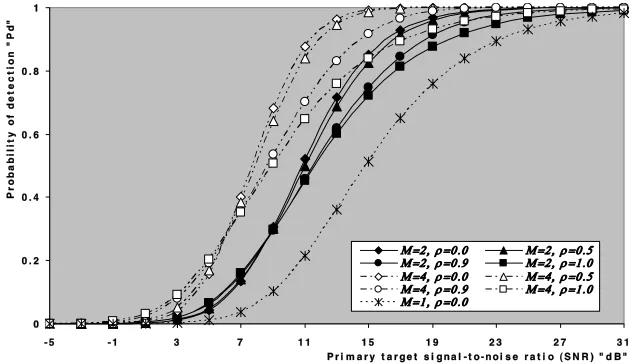
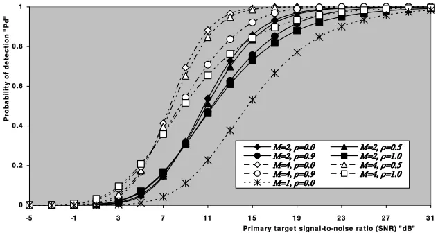
To illustrate the performance of CFAR processors for partially correlated χ2 fluctuating targets, the previous analytical expressions are programmed on a digital computer for some parameter values and the results of these programs are presented, for OSD(21), ML-OSD(10), MX-OSD(10) and MN-OSD(10) in Figs. 2–5, respectively. The abbreviation OSD(21) means the single-window OS detector with ordered-statistic parameter K of 21, while the other three abbreviations denote double-window OS detectors with symmetrical ordered-statistic parameter values of 10 (K1 = K2 = 10). The
reference window size (N) is chosen to be 24, the design Pf a is 10-6 and two values (2 & 4) for the number of integrated pulses are selected. For comparison, these figures also include the single sweep processor detection performance, relative to which we can demonstrate the processor performance improvement for M > 1. Besides the single sweep curve, there are another two families of curves. The first family indicates the detection performance of the processor under consideration for partially correlated χ2 targets (with ρs = 0, 0.5, 0.9 and 1) when the number of integrated pulses is two (M = 2). The curves of this set are labeled in the signal correlation coefficient ρs, including the SWII fluctuation model (ρs = 0) and the SWI model (ρs = 1), and the number of integrated pulses M. Examining the
0 0 .2 0 .4 0 .6 0 .8 1
-5 -1 3 7 1 1 1 5 1 9 2 3 2 7 3 1
Prim a ry t a rge t signa l-t o-noise ra t io (SN R) "dB"
P
ro
b
a
b
il
it
y
o
f
d
e
te
c
ti
o
n
"
P
d
"
Figure 2. M-sweeps homogeneous detection performance of OSD(21)
0 0 .2 0 .4 0 .6 0 .8 1
-5 -1 3 7 1 1 1 5 1 9 2 3 2 7 3 1
Prim a ry t a rge t signa l-t o-noise ra t io (SN R) "dB"
P
ro
b
a
b
il
it
y
o
f
d
e
te
c
ti
o
n
"
P
d
"
Figure 3. M-sweeps homogeneous detection performance of
ML-OS(10) for partially correlated chi-square fluctuating targets with two-degrees of freedomwhenN = 24, and Pf a = 1.0E-6.
0 0 . 2 0 . 4 0 . 6 0 . 8 1
- 5 - 1 3 7 1 1 1 5 1 9 2 3 2 7 3 1
P r i m a r y t a r g e t s i g n a l - t o - n o i s e r a t i o ( S N R ) " d B "
P
r
o
b
a
b
il
it
y
o
f
d
e
t
e
c
t
io
n
"
P
d
"
Figure 4. M-sweeps homogeneous detection performance of
0 0 .2 0 .4 0 .6 0 .8 1
-5 -1 3 7 1 1 1 5 1 9 2 3 2 7 3 1
Prim a ry t a rge t signa l-t o-noise ra t io (SN R) "dB"
P
ro
b
a
b
il
it
y
o
f
d
e
te
c
ti
o
n
"
P
d
"
Figure 5. M-sweeps homogeneous detection performance of
MN-OS(10) for partially correlated chi-square fluctuating targets with two-degrees of freedomwhenN = 24, and Pf a = 1.0E-6.
candidates of this group of curves, we observe that asρsincreases from zero to unity, more per pulse average SNR is required to achieve the same probability of detection. The second group includes the processor detection performance for partially correlated χ2 targets (with the sameρsvalues as above) when the number of postdetection integrated pulses is four (M = 4). Examining the candidates of the two families, we note that for low SNR, Pd increases monotonically with ρs, while
Pd degrades as ρs increases when the strength of the target return (SNR) is high. In addition, for fixed SNR, the processor performance improves with increasingM. However, the degradation inPdincreases with increasing ρs. This is common for the four detectors considered in this manuscript.
The nonhomogeneous performances of these processors are evaluated for a maximum allowable number of extraneous targets in each reference window. If K is chosen to be 21, for single-window detector, then the processor is able to discriminate the primary target from, at most, three outlying targets with little degradation in detection performance. For double-window processor, on the other hand, the ordered-statistic parameter K is chosen to be 10. As a result of this, the processor is able to discriminate the primary target fromtwo extraneous targets. Therefore, the double-window processor detection performance is evaluated forr1 =N1−K1 = 2 and
situation where the primary and the secondary interfering targets fluctuate in accordance with the χ2 fluctuation model with the same correlation coefficient (ρs = ρi) and of equal target return strength (INR=SNR). Figs. 6–9 illustrate the multiple-target performance of OSD(21), ML-OSD(10), MX-OSD(10) and MN-OSD(10), respectively. As in homogeneous case, the reference window size (N) is chosen to be 24, the design Pf a is 10−6 and two values (2 & 4) for the number of integrated pulses are selected. For comparison, these figures also include the single sweep processor detection performance, relative to which we can demonstrate the processor performance improvement for M > 1. Besides the monopulse curve, there are another two families of curves. These families indicate the detection performance of the considered algorithmfor partially correlated χ2 targets (with
ρs = 0, 0.5, 0.9 and 1) when the number of integrated pulses is 2 and 4, respectively. Their curves are labeled in the signal correlation coefficient ρs, including the SWII fluctuation model (ρs = 0) and the SWI model (ρs = 1), and the number of integrated pulses M. Examining the curves of this category, leads us to conclude that the behavior of the processor under consideration in the presence of extraneous targets is the same as its behavior in the absence of them with only minor degradation. In addition, as ρs increases fromzero to unity, more per pulse average SNR is required to achieve the same probability of detection.
0 0 .2 0 .4 0 .6 0 .8 1
-5 -1 3 7 1 1 1 5 1 9 2 3 2 7 3 1
Prim a ry t a rge t signa l-t o-noise ra t io (SN R) "dB"
P
ro
b
a
b
il
it
y
o
f
d
e
te
c
ti
o
n
"
P
d
"
Figure 6. M-sweeps multitarget detection performance of OSD(21)
0 0 .2 0 .4 0 .6 0 .8
-5 -1 3 7 1 1 1 5 1 9 2 3 2 7 3 1
Prim a ry t a rge t signa l-t o-noise ra t io (SN R) "dB"
P
ro
b
a
b
il
it
y
o
f
d
e
te
c
ti
o
n
"
P
d
"
1
Figure 7. M-sweeps multitarget detection performance of ML-OS(10)
scheme for partially correlated chi-square fluctuating targets with two-degrees of freedomwhenN = 24, R1 =R2= 2, and Pf a = 1.0E-6.
0 0 . 2 0 . 4 0 . 6 0 . 8 1
- 5 - 1 3 7 1 1 1 5 1 9 2 3 2 7 3 1
P r i m a r y t a r g e t s i g n a l - t o - n o i s e r a t i o ( S N R ) " d B "
P
r
o
b
a
b
il
it
y
o
f
d
e
t
e
c
t
io
n
"
P
d
"
Figure 8. M-sweeps multitarget detection performance of MX-OS(10)
0 0 .2 0 .4 0 .6 0 .8 1
-5 -1 3 7 1 1 1 5 1 9 2 3 2 7 3 1
Prim a ry t a rge t signa l-t o-noise ra t io (SN R) "dB"
P
ro
b
a
b
il
it
y
o
f
d
e
te
c
ti
o
n
"
P
d
"
Figure 9. M-sweeps multitarget detection performance of MN-OS(10)
scheme for partially correlated chi-square fluctuating targets with two-degrees of freedomwhenN = 24, R1 =R2= 2, and Pf a = 1.0E-6.
In order to demonstrate the ability of the MN-OSD in resolving multiple targets, we have assumed that all the extraneous targets are located in the lagging window only (r1 = 0, r2 = 4). Fig. 10 shows
the detection performance of different OS schemes under this condition for SWI & SWII fluctuation models. The curves of these figures are labeled in the detector under consideration and the fluctuation model whenM = 3. Fromthese results, we observe that intolerable masking of the primary target occurs in the case of OS(21), ML- and MX-OSD(10), and the masking effect is greater in the MX than in the ML scheme. The MN is the only scheme that is capable of resolving multiple targets in the reference window as long as all the interferers appear in either one of the local windows.
0 0.2 0.4 0.6 0.8 1
-5 -1 3 7 11 15 19 23 27 31
Primary target signal-to-noise ratio (SNR) "dB" Primary target signal-to-noise ratio (SNR) "dB"
Probability of detection "Pd"Probability of detection "Pd"
MN, SWII
MN, SWII MN, SWIMN, SWI MX, SWII
MX, SWII MX, SWIMX, SWI ML, SWII
ML, SWII ML, SWIML, SWI OS, SWII
OS, SWII OS, SWIOS, SWI
Figure 10. Multitarget detection performance of OS family of CFAR
schemes for chi-square fluctuating targets with two-degrees of freedom when N = 24, M = 3, R= 4,R1= 0, R2 = 4, andPf a = 1.0E-6.
1.0E-18 1.0E-18 1.0E-16 1.0E-16 1.0E-14 1.0E-14 1.0E-12 1.0E-12 1.0E-10 1.0E-10 1.0E-08 1.0E-08 1.0E-06 1.0E-06
-5
-5 -1-1 3 7 1111 1515 1919 2323 2727 3131
Interference-to-noise ratio (INR) "dB" Interference-to-noise ratio (INR) "dB"
Probability of false alarm "Pfa"Probability of false alarm "Pfa"
MN, SWII
MN, SWII MN, SWIMN, SWI MX, SWII
MX, SWII MX, SWIMX, SWI ML, SWII
ML, SWII ML, SWIML, SWI OS, SWII
OS, SWII OS, SWIOS, SWI
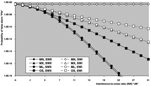
Figure 11. False alarmrate performance of OS based detectors
for chi-square fluctuating targets with two-degrees of freedomwhen
1.0E-11 1.0E-11 1.0E-10 1.0E-10 1.0E-09 1.0E-09 1.0E-08 1.0E-08 1.0E-07 1.0E-07 1.0E-06 1.0E-06
0 0 .2 0.40.4 0 .6 0.80.8 1
Correlation coefficient (rrelation coefficient (ρ) )
Probability of false alarm "Pfa"Probability of false alarm "Pfa"
MN, R1=R2=2 MN, R1=0, R2=4
MX, R1=R2=2 MX, R1=0, R2=4
ML, R1=R2=2 ML, R1=0, R2=4
OS , R=3 OS , R=4
Figure 12. Multitarget false alarm rate performance of OS family of
CFAR schemes for partially correlated chi-square fluctuating targets when N = 24, M = 3, IN R= 10 dB, and designPf a= 1.0E-6.
higher for SWI fluctuation model than their performance when the outlying targets fluctuate following SWII model. Fig. 12 depict the false alarmrate performance of the OS based detectors as a function of consecutive sweeps correlation coefficient for an interfering target strength of 10 dB and M = 3, when the spurious target returns are contained in both reference windows (r1 = r2 = 2) and in
the case where only one of the reference windows is contaminated interfering target returns (r1 = 0 & r2 = 4). The results of this
figure demonstrate our previous conclusion. In addition, the false alarmrate behavior of the OS modified versions in the case where both reference windows contaminated with interfering target returns is higher than their performance when only one of these windows is contaminated with these undesired returns. The MN-OS technique is the only one which don’t follow this rule in its reaction against outlying target returns if the desired false alarmrate is required to be constant. Moreover, the processor performance improves as the correlation coefficient among consecutive sweeps increases. Fig. 13 illustrates the required SNR for the OS based detectors to achieve an operating point of (10−6, P
d), as a function of the detection probability
4. 1 7. 7 11 .3 14 .9
0.1 0 .2 0.3 0 .4 0.5 0 .6 0. 7 0 .8 0.9
Detection probability "Pd"
Required s
ignal-to-nois
e ratio "dB"
MN, R1=
MN, R1= R2=0 MN, R1=MN, R1= R2=2 MX, R1=
MX, R1= R2=0R2=0 MX, R1=MX, R1= R2=2R2=2 ML, R1=
ML, R1= R2=0 ML, R1=ML, R1= R2=2 OS, R=0
OS, R=0 OS, R=3OS, R=3 Optimum
Optimum
Figure 13. Homogeneous and multitarget required SNR to achieve an
operating point (Pf a, Pd) of OS based schemes for fluctuating targets of SWII model when N = 24, M = 3, andPf a = 1.0E-6.
other candidates in its category, SNR to achieve a specified value forPd and the MN-OS needs the largest value of SNR to attain the same value ofPd. As a conformation of this statement, Fig. 14 shows the required SNR to attain a given operating point of (10−6, 0.9) as a function of the ranking-order parameterK, for the OS based detectors, along with the fixed threshold processor, when the radar receiver operates in an ideal environment and integrates 3 consecutive sweeps in its signal processing. Finally, the required SNR, in homogeneous as well as in multiple-target environments, against the correlation coefficient is drawn in Fig. 15) for the OS based algorithms along with the optimum scheme when the radar receiver postdetection integrates 3-pulses. The curves of this figure are labeled in the CFAR scheme,r1 and r2. The
12 12 16 16 20 20 24 24 28 28 32 32
0 2 4 6
0 2 4 6 8 1 0
Ranking-order parameter "K"anking-order parameter "K"
R
equired signal-t0-noise ratio in dBequired signal-t0-noise ratio in dB
1 2
ML-OSD, SWII
ML-OSD, SWII ML-OSD, SWIML-OSD, SWI MX-OSD, SWII
MX-OSD, SWII MX-OSD, SWIMX-OSD, SWI MN-OSD, SWII
MN-OSD, SWII MN-OSD, SWIMN-OSD, SWI Optimum, SWII
Optimum, SWII Optimum, SWIOptimum, SWI
Figure 14. Required SNR to achieve an operating point (1.0E-6, 0.9)
of OS based schemes for SWI and SWII target fluctuation models, in ideal environment, whenN = 24 and M = 3.
12 12 14 14 16 16 18 18 20 20
0 0 .2 0.40.4 0 .6 0.80.8 1
Correlation coefficient "rrelation coefficient "ρ"
R
equired signal-to-noise ratio "dBequired signal-to-noise ratio "dB
"
ML, R1=R2=0
ML, R1=R2=0 ML, R1=R2=2ML, R1=R2=2 MX, R1=R2=0
MX, R1=R2=0 MX, R1=R2=2MX, R1=R2=2 MN, R1=R2=0
MN, R1=R2=0 MN, R1=R2=2MN, R1=R2=2 OS, R=0
OS, R=0 OS, R=3OS, R=3 Optimum
Optimum
Figure 15. Homogeneous and multitarget required SNR to achieve
5. CONCLUSIONS
The problemof detecting radar targets against a background of unwanted clutter and noise is studied. We have derived exact detection probabilities for CFAR processors based, in their local noise power level estimation, on the ordered-statistic technique for partially correlated
χ2 targets. These processors include the conventional OS detector along with its modified versions which include ML-, MX- and MN-OS algorithms for their performance evaluation in the absence as well as in the presence of spurious targets. The primary and secondary interfering targets are assumed to be fluctuating in accordance with the χ2 fluctuation model with two degrees of freedom. At the limiting correlation coefficients ρ = 1 and ρ = 0, the analysis yields, respectively, the well known SWI and SWII models. The results are given in a closed formexpressions with especially simple form for a SW II fluctuation model. The analytical results have been used to develop a complete set of performance curves including the detection probability in homogeneous and multiple target situations, the variation of false alarmrate with the strength of interfering targets that may exist amongst the contents of the estimation set, and the required SNR to achieve a prescribed operating point (Pf a, Pd), as a function of the ordered-statistic parameter and correlation coefficient. As expected, lower threshold values and consequently higher detection performance is obtained as the number of postdetection integrated pulses increases. On the other hand, as the signal correlation increases fromzero to unity, more per pulse SNR is required to achieve a prescribed probability of detection. In addition, the false alarmrate increases with the signal correlation and the MN-OS scheme is the only processor that is capable of maintaining a constant rate of false alarm, irrespective to the interference level, in the case where the spurious targets are located in either one of the reference windows.
with increasing the reference window size. In addition, the likelihood that an interfering target or a spiky clutter return has entered the reference window is obviously larger for larger number of reference cells. On the other hand, once the window has been captured by an interfering target, the primary target is less suppressed when the size of the reference window is large.
When the target signal fluctuates obeyingχ2 statistics, the signal components are correlated from pulse to pulse and this correlation degrades the processor performance. A common and accepted practice in radar systemdesign to mitigate the effect of target fluctuation is to provide frequency diversity to decorrelate the signal frompulse to pulse. While this technique is effective, it requires additional system complexity and cost.
REFERENCES
1. Dillard, G. M., “Mean level detection of nonfluctuating signals,”IEEE Transactions on Aerospace and Electronic Systems, Vol. AES-10, 795–799, Nov. 1974.
2. Rickard, J. T. and G. M. Dillard, “Adaptive detection algorithm for multiple target situations,” IEEE Transactions on Aerospace and Electronic Systems, Vol. AES-13, 338–343, July 1977.
3. Nitzberg, R., “Analysis of the arithmetic mean CFAR normalizer for fluctuating targets,” IEEE Transactions on Aerospace and Electronic Systems, Vol. AES-10, 44–47, Jan. 1978.
4. El Mashade, M. B., “M-sweeps exact performance analysis of OS modified versions in nonhomogeneous environments,” IEICE Trans. Commun., Vol. E88-B, No. 7, 2918–2927, July 2005. 5. Rohling, H., “Radar CFAR thresholding in clutter and
multiple target situations,”IEEE Transactions on Aerospace and Electronic Systems, Vol. AES-19, 608–621, July 1983.
6. Kanter, I., “Exact detection probability for partially correlated Rayleigh targets,” IEEE Transactions on Aerospace and Elec-tronic Systems, Vol. AES-22, 184–196, Mar. 1986.
7. Gandhi, P. P. and S. A. Kassam, “Analysis of CFAR processors in nonhomogeneous backgrounds,”IEEE Transactions on Aerospace and Electronic Systems, Vol. AES-24, 427–445, July 1988.
8. Elias-Fuste, A. R., M. G. De Mercado, and E. R. Davo, “Analysis of some modified ordered-statistic CFAR: OSGO and OSSO CFAR,”IEEE Transactions on Aerospace and Electronic Systems, Vol. AES-26, 197–202, January 1990.
CFAR detector with noncoherent integration in homogeneous situations,”IEE Proceedings-F, Vol. 140, No. 5, 291–296, October 1993.
10. He, Y., “Performance of some generalized modified order-statistics CFAR detectors with automatic censoring technique in multiple target situations,” IEE Proc. - Radar, Sonar Navig., Vol. 141, No. 4, 205–212, August 1994.
11. El Mashade, M. B., “Performance analysis of modified ordered statistics CFAR processors in nonhomogeneous environments,”
Signal Processing “ELSEVIER”, Vol. 41, 379–389, Feb. 1995. 12. Swerling, P., “Radar probability of detection for some additional
fluctuating target cases,” IEEE Transactions on Aerospace and Electronic Systems, Vol. AES-33, 698–709, April 1997.
13. El Mashade, M. B., “Performance analysis of OS family of CFAR schemes with incoherent integration of M-pulses in the presence of interferers,” IEE Radar, Sonar Navig., Vol. 145, No. 3, 181–190, June 1998.
14. El Mashade, M. B., “Analysis of adaptive radar systems processing M-sweeps in target multiplicity and clutter boundary environments,”Signal Processing “ELSEVIER”, Vol. 67, 307–329, Aug. 1998.
15. El Mashade, M. B., “Target multiplicity performance analysis of radar CFAR detection techniques for partially correlated chi-square targets,”Int. J. Electron. Commun. AE ¨U, Vol. 56, No. 2, 84–98, April 2002.