A Novel Cascade Temperature Control System For High-Speed Heat- Air Flow Wind Tunnel

A NOVEL CASCADE TEMPERATURE

CONTROL SYSTEM FOR HIGH-SPEED HEAT-

AIR FLOW WIND TUNNEL

Kondiba R. Gayake

PG Department

M. B. E. Society’s College Of Engineering Ambajogai Ambajogai, India

Email:[email protected] m

S.S.Sankeswari

PG Department

M. B. E. Society’s College Of Engineering Ambajogai Ambajogai, India

Email:[email protected] m

Abstract — In order t o meet st ringent t emp erat ure -cont rol requirements in a high-speed airflow wind t unnel (HAWT ) for t hermal simulation under complicat ed work condit ions such as t hermal strength experiment of aero engine blade and dy namic calibration of high temperature thermal coupler, this paper proposes a novel cascade fuzzy-PID (C-Fuzzy-PID) compound control met hod for regulating the fuel-oil flow rate in the inner loop and temperature in t he outer loop. The mathematical models t hat charact eriz e t he dy namics of the heat airflow temperature in the combust or and t he fuel-oil flow rate for combust ion are derived, up on which t he imp roved PID cont rol laws for t he inner and out er loop s are described. The former emp loy s a fuz z y -PID cont roller wit h a p redictor for controlling flow rate in the inner loop, which effectively overcomes influences according to its characteristics of large inert ia and transport lag in fuel-oil sup p ly sy st em on t he t emp erat ure responses. The latter combines dist urbance comp ensat ion and a fuzzy-PID feedback law to suppress influences due to factors such as change in work conditions, disturbances, and time-varying parameter variations. T he C-Fuz z y -PID met hod has been numerically investigated by comparing simulation results against two tradit ional PID-based methods, as well as experimentally validated confirming t hat the proposed control algorit hm has st rong robust ness and excellent adapt abilit y for t emp erat ure cont rol of an HAWT .

Keywords—Cascade control, fuzzy PID, high-sp eed heat airflow Simulation, predict ive cont rol, t emp erat ure cont rol, t hermal.

I. INTRODUCTION

The high-speed airflow wind tunnel (HAWT) for thermal Simulation is an important aerospace experimental system. An HAWT that produces a uniform and controllable temperature field has been widely used in heat-strength experiments of High temperature aero engine blades and dynamic calibration of Thermal sensors. Among the challenges in developing an HAWT is the modeling of the dynamic system and the design of a controller capable of regulating temperature and fuel oil with Quick response for a wide range of the temperature. The mixing of the aviation kerosene with air and their subsequent burning in the combustor results in a complex physical field; the thermal-flied environment being simulated is a high-speed airflow of high temperature. The high

temperature airflow field is governed by the flow rate ratio between the Kerosene and the air supplied to the combustor. In practice, the Outlet airflow temperature of the HAWT for a specified airflow Speed is adjustable when conducting experiments. Thus, the output temperature of the combustor, which depends primarily on kerosene flow rate, can be theoretically controlled by precisely manipulating the flow rate of the fuel oil feeding to the combustor. However, variations in the input airflow along With inadequate fuel-oil combustion and other unknown factors Result in significant temperature fluctuations which must be considered in the controller design for regulating fuel-oil flow Rate and temperature. Prior research generally focused on the Design and control of thermal wind tunnels particularly on three Aspects: modeling and regulating the flow rate, developing a Strategy for controlling flow rate, and designing a temperature Control system for the combustion process.

II MODELING OF TEMPERATURE CONTROL SYSTEM This paper addresses problems commonly encountered in designing a controller for simultaneously regulating both the fuel-oil flow rate and the temperature of an HAWT, where the plant is characterized by a wide temperature range from 200 to 1700 ◦C and high heating rate (with temperature raised from 200 to 1700 ◦C within 30 s). Additionally, the control law must be able to deal with large thermal and flow inertia, transport time lag, and robust in the presence of significant disturbances. To effectively solve these problems, there is a need to develop a mathematical model that takes into accounts the combined dynamics of fuel-oil flow and combustion, and a method for high-performance temperature control with strong robustness. The rest of this paper offers the following.

1) The mathematical models that characterize the dynamics of fuel-oil flow and the gas temperature in the combustor for a typical HAWT are derived, which provide the essential basis for design analysis and numerical simulation.

Temperature control system of HAWT. Control loops) is presented. The inner loop incorporates a Predictive control law to overcome the influences of transport lag in the fuel-oil supply system while the outer loop is designed to suppress disturbances due to the wind speed change. Compared with the traditional PID cascade control, the C-Fuzzy-PID effectively rejects to the influence of the time lag and working conditions change.

3) The C-Fuzzy-PID method has been numerically studied by comparing simulation results against two traditional methods, PID-PID and PID-Smith, as well as experimentally evaluated demonstrating its robustness and excellent adaptability.

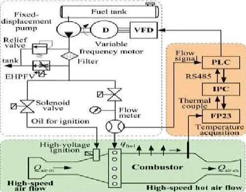
Fig.1. Temperature control system of HAWT. Fig. 2 shows the temperature control system of a typical HAWT, which consists of three subsystems; fuel-oil supply, combustion, and computer control. The fuel-oil supply subsystem adjusts the flow rate of the aviation kerosene feeding to the combustor. The combustion subsystem mixes the fogged kerosene with preheated air, burns them, and finally forms the heat air flow at a specified temperature. The control subsystem consists of a programmable logic controller (PLC) as a field controller, an industrial personal computer (IPC) as a remote controller, flow rate sensors, thermocouples, VF driver, and signal conditioning circuits. Specific control algorithms are implemented on the IPC considering that the operation ability of the PLC is limited. The PLC receives control commands from the IPC, adjusts the fuel-oil flow rate through controlling the VF motor and the proportional valve, and finally achieves the closed-loop temperature control of the overall system.

III DESIGN OF THE CONTROLLERS I .Modeling of Flow Rate in the Inner Loop

Because the fuel-oil supply system is mainly operated in the VF speed-regulating mode, the mathematical model and flow rate control strategy have been setup in this mode. The operation mode of VFD in this system is variable voltage variable frequency, the input control signal is the output voltage of the controller, and the output of the VFD is the

voltage across to the stator coil of the VF induction motor. The relationship between input and output of the VFD is linear; when not considering low frequency torque compensation, it can be expressed by

UA= KfKinvu (1)

Where UA is the output voltage of VFD

Kf is the gain between the frequency f and the input control

voltage u of the VFD, and Kinv is the voltage–frequency ratio.

Generally, the VF induction motor is operated with a constan t voltage–frequency ratio, where the electromagnetic time constant is much smaller than that of rotor dynamics. Denoting ωs as the synchronized angular frequency of the motor, Rs as the phase resistance of the stator side, and Ls and Lre as the stator inductance and equivalent rotor inductance,

respectively, and considering that the slip ratio (SL= 1− np/ns )

of the asynchronous motor is usually less than 5% under the common work conditions,

Therefore Rre ≫ sLRs, Rre ≫ sLωs(Ls+ Lre). Under the

aforementioned conditions, the torque Γe (in N ・ m) acting

on the motor shaft, which can be derived from the electromagnetic moment equation of the VF motor, can be approximately written as

Te≈

3mpU2A

WSRre

SL =3mpU

2_A

2πRre

SL (2)

Where ωs=πns/30; ns = 60f/mp; ns and ns are the actual

rotational speed and the synchronous rotational speed of the motor in revolution per minute, respectively. Substituting the expressions of sL and ns into (2) yields

Te= 3mp

2πRreKfUA− m2p 40πRreK

2_fn

p= K1UA− K2np (3)

Mechanically, the moment balance equation on the motor shaft is as follows

Te= JT

π 30

dnp dt + BT

πnp

30 +

DPPP

2πnpm

(4)

Where Pp is the output pressure of the pump in Pascal.

According to the continuity equation describing the flow rate of the volumetric chamber in the output port of the pump, and neglecting the influence of the compressibility of the fuel oil while considering that the pressure of the fuel oil is less than 1.2 MPa and the volume elastic modulus of fuel oil is larger than1.0 GPa.

Fig.2. Lumped-parameter model of a long pipeline. The output flow rate of the oil supplying the pump can be approximately written as follows:

qfuel =

1

Where qfuel is actual flow rate of oil supplying pump, m3/s.

Since the energy loss of the long fuel-oil pipeline from the pump to the combustor nozzle of the HAWT is the pressure loss, it must be modeled to account for its influences. Moreover, there are also dynamic influences of the fluid inductance and capacitance of the pipeline, as well as the throttling resistance of the nozzle in the combustor. Using the lumped parameter method [13] to model the long pipeline system (in terms of its fluid resistance R, capacitance C, and inductance L as shown in Fig. 3), the equation characterizing the transfer functions of the pipeline can be written as

[P2(s)

q2(s)

] = [1 + LCs2 −(1 + Ls + RLCs2)

−Cs 1 + RCs ] [

P1(s)

q1(s)

] (6) Where C = πd2l

4βe ; L = 4ρ_fuel

πd2_4βel ; R = R1 +R2 , R1 = 128μl

πd4 ,Ri and

R2 are the liquid resistance of the pipeline liquid or the nozzle,

respectively. The resistance RN of the nozzle. Is obtainable

from linearizing its pressure/flow rate relationship: q2=CdA√2p2/ρ_fuel (7)

Where Cd is the discharge coefficient, and A is the effective

flow area of the hole. Linearizing (7) about the operating spout pressure ̅̅̅p2 (which is generally a measurement value at

starting Frequency) leads to (8) for a constant area nozzle hole Δq2 = KcΔp2 where Kc=

CdA̅ √2ρ_fuelP̅̅̅̅2

(8)

There are six nozzles in the combustor, and the liquid resistance at the spout can be obtained according to the principle of resistance parallel as follows:

R2 = 1

6K_c =

1 ∂ p₂ 6 ∂q₂ =

√2ρ_oilP̅̅̅̅ 2

6C_dA (9)

Neglecting the compressibility of fuel oil and considering C = 0 in (6), and we can obtain.

q1 = q2 = qfuel= Pp Ls+R1+R2 (10)

Combining (1) to (10) yields a transfer function between the oil fuel flow rate qfueland the VFD input voltage u as follows:

G0 (s) =

qfuel(S)

u (S) =

b0 ω2n

s2+2 ωns+ω2n (11)

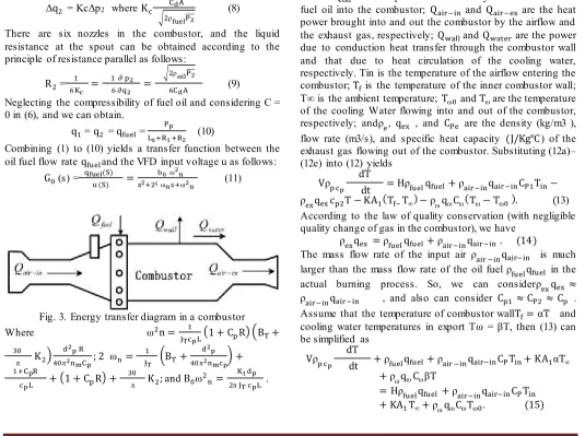
Fig. 3. Energy transfer diagram in a combustor

Where ω2_{n =} 1

JTcpL(1 + CpR) (BT+ 30

π K2)

d2_{p R}

40π2_nmCp; 2ωn= 1

JT (BT+

d2_p 40π2_nmcp) + 1+C_pR

cpL + (1 + CpR) + 30

π K2; and B0ω

2 n =

K₁d_p 2π JT cpL .

To account for the pure time delay τ existed in gear flow meter, the output flow rate qs of the flow meter is expressed by

qs(s) = e−𝛕Sqfuel(s) (11a)

II. Modeling of Temperature in the Outer Loop

Fig. 4 illustrates the energy transfer in the combustor, where the gas temperature in the combustor is the controlled variable in the outer loop. Formulated using a lumped parameter approach, the gas temperature T (assumed uniform in the combustor) is governed by the law of energy conservation given in (12) along with the individual contributions of the heat powers Q (W) defined in (12a)–(12e) in terms of temperatures (◦C):

Vρ_{p c}

p dT

dt = Qfuel+ Qair−in−

(Qair−ex+Qwater Qwall) (12)

Qfuel= Hρ_{fuel qfuel} (12a)

Qair−in=ρair−inqair−inCp1Tin (12b)

Qair−ex=ρeqexCPeT (12c)

Qwall= hAc(Tf−T ) (12d)

And

Qwater =ρωqωCω(Tω− Tω0 ) (12e)

Where Qoilthe heat power is released by combustion of the

fuel oil into the combustor; Qair−in and Qair−ex are the heat

power brought into and out the combustor by the airflow and the exhaust gas, respectively; Qwall and Qwater are the power

due to conduction heat transfer through the combustor wall and that due to heat circulation of the cooling water, respectively. Tin is the temperature of the airflow entering the combustor; Tf is the temperature of the inner combustor wall;

T∞ is the ambient temperature; Tω0 and Tω are the temperature of the cooling Water flowing into and out of the combustor, respectively; andρ_e, qex , and CPe are the density (kg/m3 ),

flow rate (m3/s), and specific heat capacity (J/Kg℃) of the exhaust gas flowing out of the combustor. Substituting (12a)– (12e) into (12) yields

Vρ_{p c}

p

dT

dt = Hρfuelqfuel+ρair−inqair−inCP1Tin−

ρ_exqexcp2T − KA1(Tf−T∞) −ρωqωCω(Tω− Tω0 ). (13)

According to the law of quality conservation (with negligible quality change of gas in the combustor), we have

ρ_exqex =ρfuelqfuel+ρair−inqair−in . (14)

The mass flow rate of the input air ρ_{air −in}qair−in is much

larger than the mass flow rate of the oil fuel ρ_fuelqfuel in the

actual burning process. So, we can considerρ_exqex ≈

ρ_air−inqair−in , and also can consider Cp1≈ CP2 ≈ Cp .

Assume that the temperature of combustor wallTf=αT and

cooling water temperatures in export Tω = βT, then (13) can be simplified as

Vρ_{p c}

p

dT

dt +ρfuelqfuel+ρair −inqair−inCPTin+ KA1αT∞ +ρ_ωqωCωβT

= Hρ_fuelqfuel+ρair−inqair−inCPTin

Because the inlet air, the inlet temperature, cooling environmental Temperature of combustor wall, and temperature of the cooling water are basically stable and can be seen as a constant in the experimental process for the certain work conditions, so the rear three items of (15) can be considered as a constant item. Taking Laplace transformation of (15) leads to the transfer function between T(s) and qoil(s)

as follows: G1 (s) =

T(S) qoil(S)

= Kp Tps + a

(16)

Where a =ρ_{air −in}qair−inCP+ KA1α+ρωqωCωβ, KP =

Hρ_fuel , and Tp = Vρp cp .

III. PROPOSED CONTROLLERS

The following two sections describe the design of the inner and outer loop controllers for regulating the fuel-oil flow rate and gas temperature, respectively

I. Design of a Flow Rate Controller in the Inner Loop

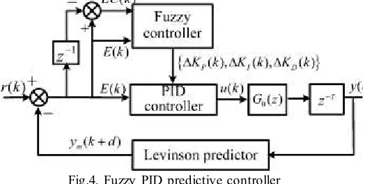
As modeled in (11) and (11a) and observed during the debugging of the system, the open-loop transfer function of the inner loop control system has a transport lag due to the flow rate sensor. In addition, the nonlinearity and uncertainty of the motor pump and pipeline also makes it difficult to achieve the desired control effects by simply using a simple fixed-gain PID controller. Fuzzy control law and fuzzy rule-based control law have been widely applied in control systems because it relaxes the accuracy requirements on the mathematical model of the plant. According to the system characteristics of a typical HAWT, an improved fuzzy-PID controller with a predictive algorithm is designed for the flow rate control in the inner loop as shown in Fig. 5. This new compound fuzzy PID control law is effective in overcoming the effects of time delay on the system. The fuzzy-PID predictive controller achieves its control performance through the combined effects of predictive control on the time-delay elimination and rule-based tuning PID gains on the improved system robustness and steady-state accuracy. As illustrated in Fig. 5, the fuzzy-PID predictive controller is implemented in three steps. In the first step, a Levinson predictor is designed to determine the output value of the future d steps from the historical data of the process output. Next, the error is computed by comparing the predicted value that is fed back

Fig.4. Fuzzy PID predictive controller

Against the reference signal. Based on the computed error and the PID gain parameters that are updated by the fuzzy

controller in real time, the final step determines the output of the PID Controller.

I. Levinson Predictor: The Levinson predictor method predicts the values of the output variables in the future d steps built upon the moving output average ym of n process historical

data. For the predictor output at kth time instant in (17), the predicted value of d step ahead is given by (18)

ym(k) = − ∑ aiy(k − i) (17) n

i=1

Where ym(k + dk) = −a1ym(k + d − 1k) − ⋯

−ap−1ym(k + 1k) − apy(k) − ⋯

− any(k + d − n) . (18)

In (17) and (18), the optimal forecasting parameters, {ai} where i = 1... n, are predetermined using a recursive least squares method

II Design of a Fuzzy-PID Controller:

The three PID gains are generally determined through empirical methods such as process reaction curve criteria; once determined, they cannot be changed throughout the controlling process. Unfortunately, these simple fixed-gain PID controllers will not guarantee the adaptability of the actual fuel supply system to the change of its working conditions. In order to have a good control effect on the flow rate, this paper enhances the PID controller with fuzzy

control which adjusts in real time the PID gains according to the state of the linguistic variables (E and EC) of the error e and the error change ec; namely, the inputs of the fuzzy PID Controllers are e and ec, and the output is the three incremental gains (ΔKp, ΔKi, and ΔKd) of the PID control law. When implementing the fuzzy PID control law, the controller inputs (e and ec) are quantified to the specified range (−5, 5), upon which the membership degree for each linguistic variable is then determined. Here, the linguis tic variable sets for the inputs and output of the fuzzy controller are chosen as {NB, NM, NS, ZO, PS, PM, PB} and expressed by {−4, −3, −2, −1, 0, 1, 2, 3, 4}. Unlike the traditional fuzzy control a Mamdanni’s rule table for fuzzy reasoning, the fuzzy rules for the fuzzy-PID controller are based on analytic formula with an adjusting factor to improve A =πr2_the

adaptability of the fuzzy rule as follows: U = [E + (1 −)EC] (19)

Fig.5. Structure of an outer loop temperature controller Where λ is the correction factor, its adjustment law is

=1E 2,1,2∈ [0,1] (20)

The fire-membership functionμ_F(u) for the fuzzy control output of each fuzzy rule can be determined as

μ_F(u) = A = ∑ ∑μ_(i,j)

5

j 5

i=1

(μ)_μi(e)μj(ec) (21)

Where μi (e), μj (ec), and μ (i,j )(u) denote the triangular membership functions. Calculation of the defuzzier formula (based on the method in [30] and [31]) can be written as

μ= ∑ μ_F( μ_k) μ_k

5

k=−5

∑ μ_F(μ_k)

5

k=−5

⁄ (22)

Where u denotes the output of the fuzzy controller after defuzzier and it has three gains of fuzzy PID.

II. Design of Temperature Controller in the Outer Loop As seen in (15), changes of the airflow, cooling water flow Rate and environment temperature would appear as disturbances in the combustor gas -temperature control system. Because the flow rate of the cooling water can be adjusted by a water supply with a regulating valve and a water pump with a fixed rotational speed in practice, the change in flow rate of the cooling water is not large. On the other hand, temperature experiments with different wind speeds at the same temperature are often needed. For example, the characteristics of a specimen at a specific temperature (say 1000◦C) must be tested for a range of wind speeds (say 0.6, 0.8, and 1 Ma). Any switch in wind speed could have a significant influence on the model and control performance of the plant; thus, the control system not only must reject any disturbances quickly to achieve accurate temperature regulation, but also overcome any impact caused by a switch of work condition; for example, a change in the airflow from 0.6 to 0.8 Ma In order to accomplish this control objective, a compound controller has been designed as shown in Fig. 6, which combines compensation for wind speed change with a fuzzy PID for temperature control. The fuzzy-PID temperature controller has the same structure for the fuzzy-PID flow rate controller in the inner loop. The compensation coefficient to reflect the Change of the wind speed is determined by combustion theory and empirical experience.

IV. SIMULATION AND RESULTS

In last chapter we discussed about different controllers part and necessity of these controller for the project here we want to do the comparative study of simulation results obtained with different controller used for avoid high temperature system. Before going to simulation results let’s see the design model for cascade controller.

I. Setting of Simulation Cases and Comparative Control Laws Comparative numerical studies were conducted using three methods.

1) C-Fuzzy-PID control law presented in the paper;

2) PID-PID cascade control law, where both the inner fuel oil flow rate loop and outer temperature loop are PID controlled; and

3) PID-Smith cascade control law, where the inner loop uses PID with a Smith predictor and outer loop adopts PID. In order to realistically simulate the wind tunnel temperature, the target temperature is initially set to 1◦C, and then increased

to 2◦C after 50 s. The C-fuzzy-PID control law is evaluated numerically in the following simulation cases.

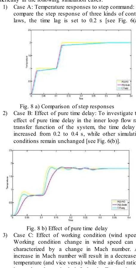
1) Case A: Temperature responses to step command: To compare the step response of three kinds of control laws, the time lag is set to 0.2 s [see Fig. 6(a)].

Fig. 8 a) Comparison of step responses

2) Case B: Effect of pure time delay: To investigate the effect of pure time delay in the inner loop flow rate transfer function of the system, the time delay is increased from 0.2 to 0.4 s, while other simulation conditions remain unchanged [see Fig. 6(b)].

Fig. 8 b) Effect of pure time delay

Fig.6 c) Effect of airflow wind speed

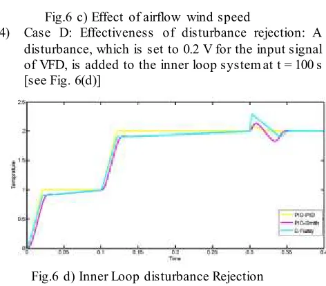
4) Case D: Effectiveness of disturbance rejection: A disturbance, which is set to 0.2 V for the input signal of VFD, is added to the inner loop system at t = 100 s [see Fig. 6(d)]

Fig.6 d) Inner Loop disturbance Rejection Fig.6 Results of comparative studies of three control laws

II Discussions of Simulation

Some observations can be made from the simulated results. As illustrated in Fig. 7(a), although all three methods yield an over damped temperature response to step changes, the fuzzy- PID method significantly improves the response time over both traditional PID-PID and PID-Smith control methods. The PID Smith has a slightly shorter settling time than that of PID-PID as it incorporates Smith predictor to compensate the time lag in the inner loop.

Fig. 6(b) illustrates that an increase in time delay causes an overshoot and lengthens the settling time. The fuzzy -PID controlled system exhibits an excellently short settling time as compared to the PID-PID and PID-Smith cascade control methods despite the fact that it yields a slightly larger overshoot in the response. It is interesting to note that that the PID-PID offers a better transient response (both overshoot and settling time) than that of the PID-Smith method in this case. This is because Smith predictor depends on an accurate mathematical model; the control performance degrades when the plant models experience parameter variations.

V. CONCLUSION AND FUTURE SCOPE I.CONCLUSIONS

A successfully developed C-Fuzzy-PID control system (with an inner flow rate and an outer temperature control loops) for temperature control of a HAWT has been presented. The plant models for both loops, which have been derived in closed form for a physical HAWT, have been shown to provide a useful basis for simulation analysis and controller design. The proposed C-Fuzzy-PID has been numerically investigated by comparing simulation results against two traditional methods; PID-PID and PID-Smith. The inner loop, which incorporates a predictive control law, effectively overcomes influences of large inertia and transport lag in fuel-oil supply system on the temperature responses. The outer loop, where the compensation coefficients of the fuzzy-PID law for temperature control can be tuned (based on combustion theory and experiences) to reflect work conditions, provides an effective means to suppress the impact caused by a change in

wind speeds. The models and the proposed C-Fuzzy-PID law have been validated experimentally showing that the proposed controller not only can realize precise temperature control, but also can quickly suppress influences caused by a change of work conditions, parameter variation, and disturbances on the plant. The temperature fluctuation of the system is less than ±7 ◦C. Simulation and experimental results have confirmed that the C-Fuzzy-PID control algorithm has strong robustness and excellent adaptability. Suggested future work may include a strict theoretical analysis of the proposed C-Fuzzy-PID for the temperature control of HAWT, which takes into account the perturbation of the controlled plant.

II.FUTURE SCOPE

Future work may lie in the investigation of c-fuzzy PID controller since the interaction among different PID may affect each other. Also, the extension to other control system control problems can be explored. We can also move towards the fuzzy controller whose results can matches with the required response in shorter time period. And concept of avoid high temperature for improvement of time and speed.

ACKNOWLEDGEM ENT

We would like to thank anonymous referees for their valuable comments and suggestions to improve the quality of paper.

BIBLIOGRAPHY

[1] S. Zhao, L. Liao, and Y. Chen, “1700◦C Hot wind tunnel for thermal Calibration,” Aviation Meas. Testing Technol., vol. 20, no. 4, pp. 3–6, Apr. 2000.

[2] T. Peng, B. Xu, and H. Yang, “Variable frequency hydraulic technology Development and research,” J. Zhejiang Univ., vol. 38, no. 2, pp. 215–221, Feb. 2004.

[3] T. Zhao, J. Zhang, and L.Ma, “On-line optimization control method based on extreme value analysis for parallel variable-frequency hydraulic pumps in central air-conditioning systems,” Building Environ., vol. 47, pp. 330– 338, Jan. 2012. [4] H. Yang, W. Sun, and B. Xu, “New investigation in energy regeneration of hydraulic elevators,” IEEE/ASME Trans. Mechatronics, vol. 12, no. 5, pp. 519–526, Oct. 2007.

[5] B. Xu, X. Ouyang, and H. Yang, “Energy-saving system applying pressure accumulators for VVVF controlled hydraulic elevators,” presented at the ASME Int.Mech. Eng.Congr. Expo.Washington, DC, USA, Nov. 16–21, 2003. [6] B. Xu, J. Yang, and Y. H. Yang, “Comparison of energy-saving on the speed control of VVVF hydraulic elevator with and without pressure.

[7] D. Hu, S. Ding, H. Zhu, B. Xu, and H. Yang, “Velocity-tracking control of the variable-speed controlled hydraulic system: Using compound algorithm of PD & feed-forward-feedback control,” in Proc. 3rd IEEE Conf. Meas. Tech. Mechatronics Autom., 2011, pp. 1109–1116.