Available Online atwww.ijcsmc.com
International Journal of Computer Science and Mobile Computing
A Monthly Journal of Computer Science and Information Technology
ISSN 2320–088X
IJCSMC, Vol. 4, Issue. 10, October 2015, pg.94 – 104
RESEARCH ARTICLE
Studying the Effect of Physical Plasma on
the Blood using Digital Image Processing
Alyaa Hussein Ali
1, Hamid
H.Murbet
2, Iman
Abdulsttar
ALhmeedi
3,
Alaa Nazar
4, Nisreen Kaleel
A.ALameerr
5¹Department of Physics Baghdad University, Iraq ²Department of Physics Baghdad University, Iraq ³Department of Physics Baghdad University, Iraq
4
Department of Physics Baghdad University, Iraq
5Department of Physics Baghdad University, Iraq
[email protected]; [email protected]
Abstract— The present work deals with physical plasma and digital image processing, it is a new way to finding the changes which occur in the blood texture as a result from exposure the blood samples to the plasma for different time; this effect can be study using the texture analysis method which is the co-occurrence matrix. It is important to mentioned that the search include four type of blood Healthy (N), Smoker (s(, Diabetes (D) and High blood pressure (P(, the healthy and high blood pressure shows a good response to the plasma while the Smoker and Diabetes shows a very small response since their blood has high viscosity.
Keywords— cold Plasma, gray level co-occurrence matrix, Statistical Feature, Image segmentation
1. INTRODUCTION
2. SECOND ORDER STATISTICAL FEATURES
Using the Statistical Textural analysis method which is the second order method depend on the gray level scale.
- Gray-Level Co-occurrence Matrix: T wo -dimensional Co -occurrence (gray -level dependence)
Matrices, proposed by Haralick in 1973, are generally used in texture analysis because they are able to cap ture the spatial dependence of graylevel values within an image. A 2D Co -occurrence Matrix, P, is an (n x n) Matrix , where n is the number of gray-levels within an image . For reasons of computational efficiency, the number of gray levels can be reduced if one chooses to bin them, thus reducing the size of the Co-occurrence Matrix. The Matrix acts as an accumulator so that P[i , j] counts the number of pixel pairs having the intensities i and j. Pixel pairs are defined by a distance and direction which can be represented by a displacement vector d =(dx,dy), where dx represents the number of Pixels moved along the x-axis, and dy represents the number of pixels moved along the y-axis of an image slice .In order to quantify this spatial dependence of gray-level values, we calculate various textural features proposed by Haralick , including Entropy, Energy, Contrast, Homogeneity and Correlation [10].
Contrast: Contrast is a measure of intensity Contrast between a pixel and its neighbour over the entire image. If the image Contrast equal 0 while the biggest value can be obtained when the image is a random intensity image and that pixel intensity and neighbour intensity are very different. The equation of the contrast is as follows [11].
Contrast=
Energy: Energy is a measure of uniformity the value is maximum when the image is constant. The equation of the contrast is as follows [11].
Energy=
Homogeneity:Homogeneity measures the spatial closeness of the distribution of the co-occurrence matrix. Homogeneity equal 0 when the distribution of the co-occurrence matrix is uniform and 1 when the distribution is only on the diagonal of the matrix. The equation of the contrast is as follows[11]:
Homogeneity=
Entropy: Entropy measures the randomness of the elements of the co-occurrence matrix. Entropy is maximum when elements in the matrix are equal to 1, while is equal to 0 if all elements are different. The equation of the contrast is as follows [11] :
Entropy=-
Correlation: is expressed by the correlation coefficient between two random variables i and j , where i represents the possible outcomes in gray tone measurement for the first element of the displacement vector, while similarly j is associated with gray tones of the second element of the displacement vector. [12]:
Correlation=
Where are standard deviation in the x and y directions, and are means.
Correlation is a measure of gray tone linear-dependencies in the image; in particular, the direction under investigation is the same as vector displacement. High correlation values (close to 1) imply a linear relationship between the gray levels of pixel pairs. Thus, GLCM correlation is uncorrelated with GLCM energy and entropy, i.e., to pixel pairs repetitions. Correlation reaches it maximum regardless of pixel pair occurrence, as high correlation can be measured either in low or in high energy situations. GLCM correlation is also uncorrelated to GLCM contrast, as high predictability of the gray level of one pixel from the second one in a pixel pair is completely independent 32 from contrast. As a limiting case of linear-dependency a completely homogeneous area may be considered, for which correlation is equal to 1[12].
3. Method and Material
A. Blood Sample
The samples aretaken forman with agebetween (30 – 40) years,blood samplesare for four cases -:Healthy case (N), Diabetes case (D), Hypertension case (P) and Smoky case (S).
B. Preparation of Blood samples
The preparation can be done by exposure each sample to the Cold Plasma starting from two second up to 50 second .Taking Image for each step ,since the exposures are two step.
4. Results and discussion
Fig. (1)(a) Shows Image of Blood samples, and Gray Image of Healthy (N) Sample at a Threshold of (100).
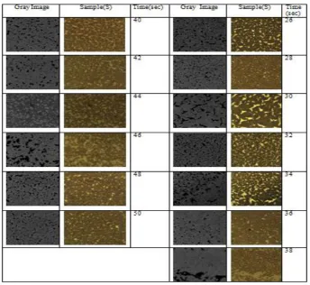
Fig(2)(a). shows Image of Blood samples, and Gray Image of Smoker (S) sample at a Threshold of (100).
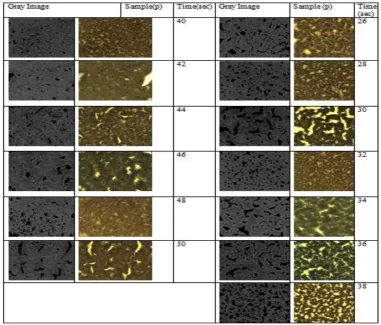
Fig(3)(a). shows Image of Blood samples, and Gray Image of a Diabetes (D) sample at a Threshold of (100 (.
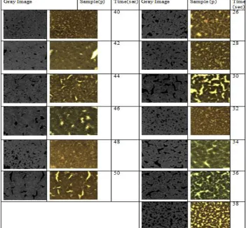
Fig(4)(a). Shows Image of Blood samples, and Gray Image of High Blood Pressure ( P) Sample at a threshold of (100).
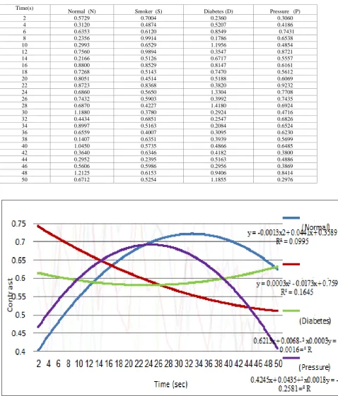
Table (1) shows Contrast values of Gray Image for Blood samples person (Healthy (N (, smoker (S) , Patients with diabetes (D) , Patients with high blood pressure (p).
TABLE (1)
SHOWS CONTRAST VALUES OF GRAY MATRIX FOR BLOOD SAMPLES PERSON (N,S,D,P).
Pressure (P) Diabetes (D)
Smoker (S) Normal (N)
Time(s) 0.3060 0.2360 0.7004 0.5729 2 0.4186 0.5207 0.4874 0.3120 4 0.7431 0.8549 0.6120 0.6353 6 0.6538 0.1786 0.9914 0.2356 8 0.4854 1.1956 0.6529 0.2993 10 0.8721 0.3547 0.9894 0.7560 12 0.5557 0.6717 0.5126 0.2166 14 0.6161 0.8147 0.8529 0.8800 16 0.5612 0.7470 0.5143 0.7268 18 0.6069 0.5188 0.4514 0.8051 20 0.9232 0.3820 0.8368 0.8723 22 0.7708 1.3304 0.5650 0.6860 24 0.7435 0.3992 0.5903 0.7432 26 0.6924 1.4180 0.4227 0.6870 28 0.4716 0.2924 0.3780 1.1880 30 0.6826 0.2547 0.6851 0.4434 32 0.6524 0.2084 0.5163 0.8997 34 0.6230 0.3095 0.4007 0.6559 36 0.5699 0.3939 0.6351 0.1407 38 0.6485 0.4866 0.5735 1.0450 40 0.3800 0.4182 0.6346 0.3640 42 0.4886 0.5163 0.2395 0.2952 44 0.3869 0.2956 0.5986 0.5606 46 0.8414 0.9406 0.6153 1.2125 48 0.2976 1.1855 0.5254 0.6712 50
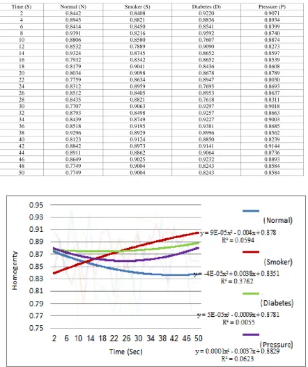
Table (2) shows Homogeneity values of Gray Image for Blood samples person (Healthy (N (, smoker (S) , Patients with diabetes (D) , Patients with high blood pressure (p).
TABLE (2)
SHOWS HOMOGENEITYVALUES OF GRAY MATRIX FOR BLOOD SAMPLES PERSON (N,S,D,P).
Pressure (P) Diabetes (D) Smoker (S) Normal (N) Time (S) 0.9071 0.9220 0.8408 0.8442 2 0.8934 0.8836 0.8821 0.8945 4 0.8399 0.8541 0.8450 0.8414 6 0.8740 0.9592 0.8216 0.9391 8 0.8874 0.7607 0.8580 0.8806 10 0.8273 0.9090 0.7889 0.8532 12 0.8597 0.8652 0.8745 0.9324 14 0.8539 0.8652 0.8342 0.7932 16 0.8608 0.8436 0.9041 0.8179 18 0.8789 0.8678 0.9098 0.8034 20 0.8030 0.8947 0.8634 0.7759 22 0.8693 0.7695 0.8959 0.8312 24 0.8637 0.8953 0.8405 0.8512 26 0.8311 0.7618 0.8821 0.8435 28 0.9018 0.9297 0.9063 0.7707 30 0.8663 0.9257 0.8498 0.8793 32 0.9003 0.9227 0.8749 0.8439 34 0.8685 0.9381 0.9195 0.8518 36 0.8562 0.8996 0.8929 0.9296 38 0.8239 0.8850 0.9124 0.8123 40 0.9144 0.9141 0.8973 0.8842 42 0.8736 0.9064 0.8862 0.8911 44 0.8893 0.9232 0.9025 0.8649 46 0.8584 0.8243 0.9004 0.7749 48 0.8584 0.8243 0.9004 0.7749 50
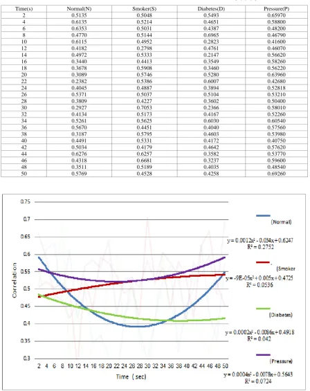
Table (3) shows Correlation values of Gray Image for Blood samples person (Healthy (N (, smoker (S) , Patients with diabetes (D) , Patients with high blood pressure (p).
TABLE (3)
SHOWS CORRELATION VALUES OF GRAY MATRIX FOR BLOOD SAMPLES PERSON (N,S,D,P).
Pressure(P) Diabetes(D) Smoker(S) Normal(N) Time(s) 0.65970 0.5493 0.5048 0.5135 2 0.58800 0.4651 0.5214 0.6135 4 0.48200 0.4387 0.5031 0.6353 6 0.46790 0.6965 0.5144 0.4770 8 0.41600 0.2823 0.4952 0.6115 10 0.46070 0.4761 0.2798 0.4182 12 0.56620 0.2147 0.5333 0.4972 14 0.58260 0.3549 0.4413 0.3440 16 0.56220 0.3460 0.5908 0.3678 18 0.63960 0.5280 0.5746 0.3089 20 0.42680 0.6007 0.5386 0.2382 22 0.52818 0.3894 0.4887 0.4045 24 0.53210 0.5104 0.5037 0.5371 26 0.50400 0.3602 0.4227 0.3809 28 0.58010 0.2366 0.7053 0.2927 30 0.52260 0.4167 0.5173 0.4134 32 0.60540 0.6030 0.5625 0.5261 34 0.57560 0.4040 0.4451 0.5670 36 0.53980 0.4603 0.5795 0.3187 38 0.40750 0.4172 0.5331 0.4491 40 0.57620 0.4642 0.4179 0.5034 42 0.53770 0.3582 0.6257 0.6276 44 0.59600 0.3237 0.6681 0.4318 46 0.48540 0.4035 0.5189 0.3511 48 0.69260 0.4258 0.4528 0.5769 50
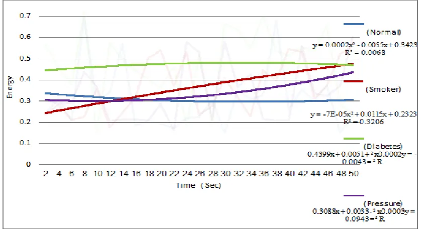
Table (4) shows Energy values of Gray Image for Blood samples person (Healthy (N (, smoker (S) , Patients with diabetes (D) , Patients with high blood pressure (p).
TABLE (4)
SHOWS ENERGY VALUES OF GRAY MATRIX FOR BLOOD SAMPLES PERSON (N,S,D,P). Pressure(P) Diabetes(D) Smoker(S) Normal (N) Time(S) 0.3033 0.56610 0.2369 0.2423 2 0.2873 0.45790 0.2827 0.3121 4 0.2904 0.37960 0.2096 0.2109 6 0.4390 0.72480 0.2248 0.6977 8 0.3706 0.15340 0.3548 0.2972 10 0.2047 0.57500 0.1767 0.3437 12 0.2147 0.49970 0.2450 0.5695 14 0.2129 0.44020 0.3212 0.1841 16 0.2071 0.40330 0.5026 0.2087 18 0.2857 0.36330 0.5418 0.1914 20 0.1615 0.46320 0.3730 0.1719 22 0.5810 0.18450 0.5307 0.2209 24 0.5321 0.51790 0.2340 0.2269 26 0.2126 0.19370 0.2757 0.3047 28 0.5801 0.66650 0.4079 0.1514 30 0.3655 0.63650 0.3169 0.3520 32 0.4261 0.55050 0.2288 0.3088 34 0.2158 0.70170 0.4451 0.3273 36 0.2080 0.53650 0.3959 0.6799 38 0.2066 0.51250 0.5462 0.2622 40 0.5572 0.55505 0.5312 0.3557 42 0.3355 0.53620 0.3124 0.3009 44 0.3248 0.65940 0.3753 0.3740 46 0.3736 0.27990 0.5217 0.1536 48 0.6024 0.23960 0.5623 0.2296 50
Fig(5,6,7,8) show the statistical features with time .Fig (5) which is the contrast with time shows that for the Normal and the Pressure case the Contrast curve increase with time which is between (24 and 30 second ),while for the Smoker and Diabetes case the carve behaviour inverses .It’s value decrease with time to accretion second then the curve increased roughly .
Fig.(6) represented the Homogeneity with time curve ,the Diabetes shows very small response to the Plasma effect while the Smoker shows small increase with time .The Pressure and Normal case decrease with time , since the Homogeneity gives indication about the purity of the tissue .
Fig.(7) which the Correlation with time it’s behaviour in opposite to the Contrast and this can observed from the graph the normal and pressure case decrease with time for a certain time .while the Smoker curve shows small increasing with time .
Fig.(8) which the Energy time curve the Diabetes and the Normal case shows no response to the effect of Plasma while the Smoker curve increase with time, and the Pressure case shows very small response to the Plasma effect .
5. Conclusions
The concluding can be expressed as follows:
1. The Contrast values changes significantly in the samples (N,P) , and changes little in the samples (S,D).
2. The values of both the Homogeneity and the Correlation changes significantly in the samples of (N,P), and changes very little almost unnoticed in (S,D) samples .
3. The Energy values changes little in (S,P) samples , and does not change in (N,D) samples .
From the above it can be concluded that the effect of the Cold Plasma in the Blood samples of both the smokers and people with Diabetes mellitus was very limited and does not show a clear change in the properties of Image Texture , but its effect on the Blood samples of the healthy person , and the person with High Blood Pressure (hypertension) can be observed from the change occurred in the Image Texture .
REFERENCES
[1] Vijay Nehra ,Ashok Kumar and H K Dwivedi'',Atmospheric Non-Thermal Plasma Sources .''International
Journal of Engineering ,Vol : ) Issue (1), 2007. 2(
[2] Arben Kojtari1, Utku K Ercan2, Josh Smith1, Gary Friedman3, Richard B Sensenig2, Somedev Tyagi,
Suresh G Joshi, Hai-Feng Ji and Ari D Brooks , Nanomedine Biotherapeutic Discov 2013, 4:1.
[3] Janga D. I., Leea S. B., Moka,c Y. S., Jangb D. L., International Journal of Chemical and Environmental
Engineering . June 2013, Volume 4, No.3.
[4] Garcia-Alcantara E, Lopez-Callejas R, Morales-Ramirez PR, Pena-Eguiluz R,Fajardo-Munoz R,
Mercado-Cabrera A, Barocio SR, Valencia-Alvarado R, Rodriguez-Méndez BG, Munoz-Castro AE, de la
Piedad-Beneitez A, Rojas-Olmedo IA, Arch Med Res, 2013, 44(3):169–177.
[5] Fridman G, Friedman G, Gutsol A, Shekhter AB, Vasilets VN, Fridman A, Plasma Processes Polym 2008,
5:503–533..
[6] Chiper AS, Chen W, Mejlholm O, Dalgaard P, Stamate E, Plasma Sources Sci Technol 2011, 20:10.
[7] Chiang MH, Wu JY, Li YH, Wu S, Chen SH, Chang CL, Surf Coat Technol 2010, 204:3729–3737.
[8] Wagner HE, Brandenburg R, Kozlov KV, Sonnenfeld A, Michel P, Behnke JF, Vacuum 2003, 71:417– 436.
[9] Kogelschatz U, Hirth M, Eliasson B, J Phys D: Appl Phy 1987, 20:1421–1437.
[10] David A. Clausi . "An analysis of co-occurrence texture statistics as a function of gray level
quantization" .Can. J. Remote Sensing, Vol. 28, No.1, pp. 45-62., 2002
[11] Laws K.," Textured image segmentation". Ph.D. dissertation, University of Southern California.1980
[12] Guneet Saini ." Texture Analysis Of CT Scan Images".Thesis submitted in partial fulfillment of the