Available Online at www.ijcsmc.com
International Journal of Computer Science and Mobile Computing
A Monthly Journal of Computer Science and Information Technology
ISSN 2320–088X
IMPACT FACTOR: 5.258IJCSMC, Vol. 5, Issue. 7, July 2016, pg.186 – 193
Traffic flow Prediction with Big Data
Using SAE’S Algorithm
S.Piramu Kailasam
(Ph.d), K.Aruna Anushiya, Dr. M.Mohammed Sathik
¹Research Scholar, Bharathiar University, India ²Assistant Professor, MSU College, India
3
Principal, Sadakathullah Appa College, Tirunelveli, India
1
[email protected]; 2 [email protected]
Abstract— Intelligent transportation system is accurate and time based traffic flow information to do best performance . Last few years, traffic data have been huge, existing system used weak traffic prediction models which is unsatisfied. The proposed system is using novel deep learning based traffic flow prediction method, which involves the spatial and temporal correlations inherently. A stack autoencoder model is used to learn generic traffic flow features and it is trained in a greedy layerwise pattern. This is the first time that a deep architecture model is proposed using autoencoders to represent traffic flow features for prediction.
Keywords— Deep learning, stacked autoencoders (SAEs), traffic flow prediction.
I. INTRODUCTION
The traffic flow information is [1] the potential to help road users, which make better travel decisions in traffic congestion and reduce carbon emissions. This will improve traffic operation efficiently. Now days transportation management system and control becomes more complicated data driven. The most of the Traffic flow predication system method is used shallow traffic model which are unsatisfied. Deep learning , which is a type of machine learning method, has a lot of interest academic and industrial level
.
Deep learning algorithms use multiple-layer architectures to extract inherent features in data from the lowest to the highest level using deep learning algorithm. Without prior knowledge, we can represent the traffic feature which has good performance in traffic flow prediction.
II. LITERATURE REVIEW
A Traffic flow prediction is a key functional component in ITSs. A countable traffic flow prediction models have been developed to assist in traffic management .These models will control and improving transportation efficiency ranging from route guidance and vehicle routing . The traffic flow can be considered a temporal and spatial process. The traffic flow prediction problem can be stated as follows. Let Xt i denote the observed traffic flow quantity during the tth time interval at the ith observation location in a transportation network. Given a sequence {Xt i} of observed traffic flow data, i = 1, 2, . . . , m, t = 1, 2, . . . , T , the problem is to predict the traffic flow at time interval (t+Δ) for some prediction horizon Δ. As early as 1970s, the autoregressive integrated
flow forecasting in [23]. An online learning weighted support vector regression (SVR) was presented in [24] for short-term traffic flow predictions. Various ANN models were developed for predicting traffic flow. It is difficult to say that one method is clearly superior over other methods in any situation. One reason for this is that the proposed models are developed with a small amount of separate specific traffic data, and the accuracy of traffic flow prediction methods is dependent on the traffic flow features embedded in the collected spatiotemporal traffic data. Moreover, in general, literature shows promising results when using NNs, which have good prediction power and robustness. Although the deep architecture of NNs can learn more powerful models than shallow networks, existing NN-based methods for traffic flow prediction usually only have one hidden layer. It is hard to train a deep-layered hierarchical NN with a gradient-based training algorithm. Recent advances in deep learning have made training the deep architecture feasible since the breakthrough of Hinton , and these show that deep learning models have superior or comparable performance with state-of-the-art methods in some areas. In this paper, we explore a deep learning approach with SAEs for traffic flow prediction.
III.METHODOLOGY
In proposed system SAE’s model is introduced SAE is Stacked Autoencoder. The SAE is an Neural network
that attempt to reduce its input. Fig.1 gives the details of auto encoder, which has one input layer, one hidden layer and one output layer. A set of training samples
{x(1), x(2), x(3), . . .}, where x(i) ∈ Rd, an autoencoder first encodes an input x(i) to a hidden representation
y(x(i)) based on (1), and then it decodes representation y(x(i)) back into a reconstruction z(x(i)) computed as (2). y(x) =f(W1x + b) (1)
z(x) =g (W2y(x) + c) (2)
where
W1 is a weight matrix,
bis an encoding bias vector, W2 is a decoding matrix, and cis a decoding bias vector.
Fig.2. Layerwise training of SAEs.
Where
γ is the weight of the sparsity term, ρ is a sparsity parameter
ρj = average activation of hidden unit
KL(ρ_ˆρj) - is the Kullback–Leibler (KL) divergence
SAEs
A SAE model is created by stacking autoencoders to form a deep network by taking the output of the autoencoder found on the layer below as the input of the current layer .The l- layers in SAE, the first layer is trained as an autoencoder, with the training set as inputs. After obtaining the first hidden layer, the output of the
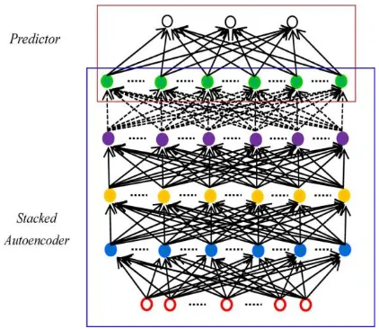
kth hidden layer is used as the input of the (k + 1)th hidden layer, multiple autoencoders can be stacked hierarchically. This is shows in Fig. 2 By using the SAE network for traffic flow prediction, we need to add a standard predictor on the top layer. In this paper, we put a logistic regression layer on top of the network for supervised traffic flow prediction. The SAEs plus the predictor comprise the whole deep architecture model for traffic flow prediction.
This is showed in Fig. 3.
Fig. 3. Deep architecture model for traffic flow prediction. A SAE model is used to extract traffic flow features, and a logistic regression layer is applied for
prediction.
C. Training Algorithm
by supervised training.
5) Fine-tune the parameters of all layers with the BP method in a supervised way.
This procedure is summarized in Algorithm 1.
Algorithm 1. Training SAEs Given training samples X and the desired number of hidden
layers l,
Step 1) Pretrain the SAE
— Set the weight of sparsity γ, sparsity parameter ρ, initialize weight matrices and bias vectors randomly.
— Greedy layerwise training hidden layers.
— Use the output of the kth hidden layer as the input of the (k + 1)th hidden layer. For the first hidden layer, the input is the training set.
— Find encoding parameters for the (k + 1)th hidden layer by minimizing
the objective function.
Step 2) Fine-tuning the whole network
— Initialize randomly or by supervised training like ,
— Use the BP method with the gradient-based optimization technique to change the whole network’s parameters in a top–down fashion.
Data Description
The proposed deep architecture model was applied to the data collected from the Caltrans Performance Measurement System (PeMS) database as a numerical example. The traffic data are collected every 30 s from over 15000 individual detectors, which are deployed statewide in freeway systems . The collected data are aggregated 5-min interval each for each detector station. In this paper, the traffic flow data collected in the weekdays of the first three months of the year 2013 were used for the experiments. The data of the first two months were selected as the training set, and the remaining one month’s data were selected as the testing set.
For freeways with multiple detectors, the traffic data collected by different detectors are aggregated to get the average traffic flow of this freeway. Note that we separately treat two directions of the same freeway among all the freeways, in which three are one-way. Fig. 4 is a plot of a typical freeway’s traffic flow over time for weekdays of some week.
Experiments :
we use three performance indexes, which are the mean absolute error (MAE), the mean relative error (MRE), and the RMS error(RMSE).
RESULT
We compared the Index of Performance
where fi is the observed traffic flow, and ˆ fi is the predicted traffic flow.
TRAFFIC FLOW ANALYSIS PATTERN FOR WEEKDAYS
HOURS(X)
NO.OF VEHICLES(Y) ON MONDAY
NO.OF VEHICLES(Y) ON TUESDAY
NO.OF VEHICLES(Y)
ON WEDNESDAY
NO.OF VEHICLES(Y)
ON THURSDAY
NO.OF VEHICLES(Y)
ON FRIDAY
0 100 100 100 105 120
2 50 50 50 50 80
4 60 60 70 55 80
6 400 380 403 400 380
8 590 550 550 600 580
10 450 450 480 502 40
12 490 500 500 500 520
14 505 550 550 550 570
16 590 590 580 580 560
18 550 510
550 570 530
20 400 400 475 500 450
22 250 300
280 350 350
WEDNESDAY TRAFFIC FLOW ANALYSIS
FRIDAY TRAFFIC FLOW ANALYSIS
IV.CONCLUSIONS
The Era of Big data is an urgent need for advanced data acquisition, management and analysis. In this paper we have presented the concept of big data and highlighted the big data value chain. The proposed method discovered the traffic flow feature representation as the nonlinear spatial and temporal correlations from the traffic data. We used the greedy layerwise unsupervised learning algorithm to pretrain the large network and improve the prediction performance. We assessed the performance of the proposed method and compared with BP NN, RBF NN, RW and SVM models and the result show that the proposed method is better than the other method. Future work, it would be interesting to find deep learning algorithm for traffic flow prediction.
he version of this template is V2. Most of the formatting instructions in this document have been compiled by Causal Productions from the IEEE LaTeX style files. Causal Productions offers both A4 templates and US Letter templates for LaTeX and Microsoft Word. The LaTeX templates depend on the official IEEEtran.cls and IEEEtran.bst files, whereas the Microsoft Word templates are self-contained. Causal Productions has used its best efforts to ensure that the templates have the same appearance.
R
EFERENCES
[1] N. Zhang, F.-Y. Wang, F. Zhu, D. Zhao, and S. Tang, ―DynaCAS: Computational experiments and
decision support for ITS,‖ IEEE Intell. Syst.,vol. 23, no. 6, pp. 19–23, Nov./Dec. 2008.
[2] J. Zhang et al., ―Data-driven intelligent transportation systems: A survey,‖IEEE Trans. Intell. Transp. Syst., vol. 12, no. 4, pp. 1624–1639, Dec. 2011.
[3] M. S. Ahmed and A. R. Cook, ―Analysis of freeway traffic time-series data by using Box–Jenkins techniques,‖ Transp. Res. Rec., no. 722, pp. 1–9,1979.
[4] M. Levin and Y.-D. Tsao, ―On forecasting freeway occupancies and volumes,‖Transp. Res. Rec., no. 773,
pp. 47–49, 1980.
[5] M. Hamed, H. Al-Masaeid, and Z. Said, ―Short-term prediction of traffic volume in urban arterials,‖ J. Transp. Eng., vol. 121, no. 3, pp. 249–254,May 1995.
[6] M. vanderVoort, M. Dougherty, and S. Watson, ―Combining Kohonen maps with ARIMA time series
models to forecast traffic flow,‖ Transp.Res. C, Emerging Technol., vol. 4, no. 5, pp. 307–318, Oct. 1996.
[7] S. Lee and D. Fambro, ―Application of subset autoregressive integrated moving average model for
short-term freeway traffic volume forecasting,‖Transp. Res. Rec., vol. 1678, pp. 179–188, 1999.
[8] B. M. Williams, ―Multivariate vehicular traffic flow prediction—Evaluation of ARIMAX modeling,‖
Transp. Res. Rec., no. 1776, pp. 194–200, 2001.
[9] Y. Kamarianakis and P. Prastacos, ―Forecasting traffic flow conditions in an urban network—Comparison
of multivariate and univariate approaches,‖Transp. Res. Rec., no. 1857, pp. 74–84, 2003, Transporation Network Modeling 2003: Planning and Administration.