Millennium Review for submission to Atmospheric Environment R N Colvile, E J Hutchinson, J S Mindell*, R A Warren T H Huxley School, Imperial College, London SW7 2BP, UK.
*Department of Epidemiology and Public Health, Imperial College, London W2 1PG, UK.
Abstract
Transport first became a significant source of air pollution after the problems of sooty smog from coal combustion had largely been solved in western European and North American cities. Since then, emissions from road, air, rail and water transport have been partly responsible for acid deposition, stratospheric ozone depletion and climate change. Most recently, road traffic exhaust emissions have been the cause of much concern about the effects of urban air quality on human health and tropospheric ozone production. This article considers the variety of transport impacts on the atmospheric environment by reviewing three examples: urban road traffic and human health, aircraft emissions and global atmospheric change, and the contribution of sulphur emissions from ships to acid deposition. Each example has associated with it a different level of uncertainty, such that a variety of policy responses to the problems are appropriate, from adaptation through precautionary emissions abatement to cost-benefit analysis and optimised abatement. There is some evidence that the current concern over the transport contribution to urban air quality is justified, but aircraft emissions should also give cause for concern given that air traffic is projected to continue to increase. Emissions from road traffic are being reduced substantially by the introduction of technology especially three-way catalysts and also, most recently, by local traffic reduction measures especially in western European cities. In developing countries and Eastern Europe, however, there remains the possibility of great increase in car ownership and use, and it remains to be seen whether these countries will adopt measures now to prevent transport-related air pollution problems becoming severe later in the 21st century.
Key words: Vehicle emissions, Aerosol urban, Health impact, Ship emissions, Aircraft emissions
1 Introduction
Transport is widely recognised to be a significant and increasing source of air pollution world wide. Several previous reviews have focused on individual modes of transport and/or single environmental impacts of transport. For example, OECD (1988) briefly considers regional and global impacts of transport emissions of air pollution, but is mostly concerned with the impact of emissions on local urban air quality, and considers only road transport. The Third International Symposium on Transport and Air Pollution (Joumard, 1996) also has an emphasis on road traffic and urban air quality, but the Special Edition of Science of the Total Environment presenting highlights of the symposium also includes a few papers covering air and sea transport. Joumard comments on the value of the contributions from developing countries including Africa and Latin America; a review of road transport emissions and their impact on the environment at all scales from local to global was also published a couple of years earlier by Faiz (1993). One of the most comprehensive recent reviews of the environmental impacts of transport is that of the Royal Commission on Environmental Pollution (Houghton, 1994). This report includes a section on air transport, and the treatment of surface transport includes freight as well as passenger, rail as well as road. Shipping is mentioned briefly by reference to other work, especially Donaldson (1994). Urban air quality and global climate change are identified as major issues, but regional air quality, acidification, noise and impacts other than air pollution emissions are also considered. There is an emphasis on assessing possible solutions to environmental problems caused by transport, concluding with an exhaustive list of recommendations; these are for the UK, but the perspective is international. An update three years later (Houghton, 1997) has a narrower scope, restricting itself to inland surface transport, motivated by a concern that there was still too little action to limit the environmental impact of road traffic despite much debate on the subject having been stimulated. Most recently, the Intergovernmental Panel on Climate Change (Penner et al., 1999) has published a major report focusing on air transport and the global environment, in contrast to the emphasis on road transport in much of the earlier literature.
In addition to these reviews, a number of papers attempting to quantify the environmental cost of transport necessarily include a concise review of the subject, but since preparation of a complete impact valuation is a huge interdisciplinary task it is more common to consider road transport alone even if an attempt is made to quantify all its impacts. We will not attempt a survey of this area of economics here, although one example (Eyre et al., 1997), will be cited later as an example where the authors include a greater than usual emphasis on atmospheric science.
soon to be followed by similar developments in diesel emissions control, is arguably the biggest exercise ever carried out in the application of end-of-pipe technology for the abatement of air pollution emissions from any type of source, certainly if the scale of the exercise is measured in terms of the number of individual people affected world-wide. Nearly every family in the industrialised countries is already involved and increasing numbers of people in developing countries and the former Soviet Bloc are following, as the motor car is one of the great icons of 20th century capitalism. In this review, we will ask the question, is the impact of road traffic emissions on urban air quality really currently the biggest issue concerning transport emissions of air pollution, and is it likely to remain so beyond the first few years of the 21st century? We will see that the extent to which we understand the relevant atmospheric science is different for each single impact of individual modes of transport that we will consider. Since it is very difficult to assess the relative severity of disparate impacts of air pollution emissions, this variability in the completeness of our understanding of the science is also having an impact on how different modes of transport are becoming subject to legislation, economic incentives to control emissions, and voluntary action to protect the environment.
The review starts with a summary of air pollution emissions from transport, by presenting an overview of how emissions inventories are compiled and used (section 2), with particular emphasis on road traffic emissions. This is followed by a brief survey of the impacts of these emissions on the environment and society, presented chronologically to indicate that concern for the environmental impact of transport has evolved over the past three decades (section 3). The three selected examples of impacts of air pollution emissions from individual transport sectors are presented in section 4, from which it is possible to see how some of the lessons learnt in trying to control emissions from road transport might be applied to other modes in future, and vice versa. The review concludes with a discussion of whether the current preoccupation with road transport and urban air quality is likely to be long lasting given the magnitude of the impact and the level of uncertainty in our ability to quantify it, from which recommendations for further work to support future sustainable integrated transport systems are drawn.
2 Overview of transport contribution to emissions
2.1. Air pollutants emitted by transport sources
With a few exceptions, all modes of transport emit air pollution from the combustion of liquid fossil fuel. Most transport sources today therefore emit similar pollutants, although the relative abundance of these varies depending on the exact composition of the fuel and details of the combustion conditions.
The most significant transport emissions to the atmosphere by mass are carbon dioxide (CO2) and water vapour (H2O)
from the complete combustion of the fuel. Some transport power sources achieve almost complete combustion by ensuring there is plenty of excess air, as in a diesel engine or a lean-burn petrol engine. A feature that distinguishes other mobile combustion sources from almost all stationary sources, however, is that combustion is incomplete, and a small fraction of the fuel is oxidised only to carbon monoxide (CO) with some volatile hydrocarbons also emitted as vapour in the exhaust and carbonaceous particles from incompletely burnt fuel droplets. The particles from a modern diesel engine, after modification by coagulation and other processes that occur in the first few seconds after emission, have a bimodal size spectrum with a large number of particles below 20 nm in size and another mode between about 30 and 100 nm (Shi, Harrison and Brear, 1999), with approximately equal total mass in each mode.
In addition to the mixture of hydrocarbons, all fuels contain some impurities (with the possible exception of hydrogen obtained from a fuel cell, and the lightest hydrocarbon fuels such as methane which are available with very low levels of impurities). Sulphur is oxidised mostly to sulphur dioxide (SO2) on combustion, and sometimes to sulphate which can
assist in the nucleation of particles in the exhaust. Several other impurities such as vanadium in oil do not burn or have combustion products that have a low vapour pressure and so contribute further to particle formation. The organic lead compounds that are still added to high octane petrol only in parts of Africa and Asia, to prevent premature combustion, also form particles in the exhaust. Finally, at the high combustion temperatures of most transport sources of air pollution, atmospheric nitrogen (N2) is oxidised to nitric oxide (NO) and small quantities of nitrogen dioxide (NO2), in
addition to smaller quantities from nitrogen-containing impurities in the fuel. Nitrous oxide (N2O) is emitted only in small
quantities from the combustion process, but is somewhat more abundant in the exhaust of cars fitted with catalytic converters.
2.2. Life-cycle analysis of emissions from transport
The air pollution emissions generated during use of any form of transport are only a part of the total amount of air pollution generated by transport-related activity. The techniques of Lifecycle Analysis (LCA) (ISO, 1997) can be used to identify which stage in the production, use and disposal of a given transport technology is responsible for the most significant atmospheric emissions. For the majority of examples, most of the emissions occur at the time and place of transport use. For example, 60 to 65% of lifecycle greenhouse gases from a petrol-engined car are CO2 exhaust
emissions during use with a further 10% being non-CO2 exhaust emissions during use. The remainder is 10%
associated with the car’s manufacture (mostly energy use), and a further 15 to 20% emitted during extraction, refinery and transport of its fuel (OECD, 1993). It should be noted, however, that this calculation excludes significant quantities of CO2 that are emitted in the production of materials to construct transport infrastructure such as roads and bridges,
especially concrete. For hydrocarbon emissions, the pre-use part of the fuel life-cycle is even more important (neglecting, for this example, the fact that different hydrocarbons emitted at different locations can have very different impacts), as shown in Fig. 1 (Gover et al., 1996), and other volatile organic compounds are emitted on evaporation of solvents during painting the bodywork as well as evaporation from the fuel tank and parts of some older engines when the vehicle is not in use. For airbags and air conditioning units, the major emission of the gases contained within them is on disposal at the end of their life.
urban transport. Coal-fired generation of electricity tends to produce a larger amount of SO2 per unit mass of fuel than
combustion of oil by stationary or mobile sources, because the amount of sulphur in coal is often higher (1 to 6% by mass) than in oil, and there is no refining process where sulphur can be removed; natural gas for electricity generation or used in a mobile source has negligible levels of sulphur, the same as the most recent clean automotive fuels. Nuclear generation of electricity has the potential to emit zero levels of air pollution, although the Chernobyl accident illustrated that this is not always achieved in practice. Hydroelectric power’s only emissions are during construction and demolition of the plant, and wind power is similar with the addition of noise emissions during use.
2.3. Quantification of emissions from transport
Atmospheric emissions can be quantified by adopting so-called “top-down” or “bottom up” methodology to generate an emissions inventory.
The top-down approach starts with data describing total polluting activity throughout the whole geographical area of interest, such as total national petrol sales for calculation of road transport emissions. This is related to the magnitude of the associated air pollution source by means of an emissions factor that can be obtained by laboratory measurement of a representative sample of engines or vehicles under simulated typical operating conditions, for example average NOx emission per litre of petrol consumed. It is important to allow for the fact that engines in use are typically not maintained to the manufacturers’ specified standards for emissions minimisation, and this is now taken into account for determination of road transport emissions though still not for some aircraft emissions. Spatial disaggregation of a top-down emissions inventory is then performed, if required, by assuming local emissions are proportional to some other variable that can reasonably be assumed to have a similar geographical distribution to that of the polluting activity, for example population density or length of road per unit area of land.
The bottom-up approach is different in that it starts with geographically resolved data, for example traffic flow on an individual length of road. For some sources (usually the larger stationary ones) emissions data are determined directly by measurement of each individual source. More usually however, especially for transport emissions where a large number of small individual sources are involved, emissions factors again need to be used, for example average emissions of NOx per vehicle per kilometre driven. Total emissions for a geographical area of interest can then be obtained by summing all the individual contributions.
The top-down and bottom-up methods invariably give different total emissions, as each is subject to different sources of error (for example, Samaras, Kyriakis and Zachariadis, 1995). For road traffic, annual emissions for a typical whole city where activities are rather well characterised can be determined to within a factor of two or better using either method, while emissions from a smaller part of the city or a shorter averaging time, such as a single road during a specific hour, are generally known rather less accurately, with a more than factor of ten overestimation or underestimation being quite common. A “bottom-up” emissions inventory inherently suffers from requiring very large amount of data, such that there is a tendency to make several assumptions and approximations. For example, traffic surveys quantifying the number of vehicles on every road in a town or city are usually taken manually (although video cameras can now determine vehicle type by reading the registration plate), so each road will be sampled no more than a few days per year and average factors applied to relate this to weekends, nights and other seasons. Automatic traffic counts rarely give any information about vehicle type. Computational models of traveller behaviour can be used to fill in data gaps on major roads, but are typically designed to study peak flow not daily or total emissions, and also might consider all vehicles as multiples of the number of passenger cars, still therefore needing factors to be applied to get hour-by-hour flows 365 days per year broken down into vehicle types for the quantification of air pollution emissions.
A convenient and regularly updated review of emissions factors for Western cities and inventory construction methodology is maintained by the London Research Centre (LRC, 1999), including data from the European Community DRIVE programme (Jost et al., 1992) and information from USEPA (1999). Fig. 2 shows data from two examples of emissions inventories: an urban inventory for fine particles (Buckingham et al., 1997), apparently showing a large contribution from diesel-engined road transport which will be discussed further below, and an older national inventory for carbon dioxide (ERR (1990) cited in Whitelegg (1993)) showing a significant contribution from transport, including air transport for which emissions are expected to increase while others decrease (Penner et al., 1999).
Emissions inventories can be valuable in providing a first estimate of the contribution of transport to air pollution emissions compared with other activity, or the relative contribution of alternative modes of transport when designing sustainable integrated transport systems. There are two respects, however, in which doing this can result in erroneous analysis. Firstly, different types of source of a given pollutant might have very different source-receptor relationships. This is unimportant for well-mixed pollutants such as CO2, for which the total global concentration is of interest, but in an
urban area emissions from vehicle exhausts are much closer to human receptors than tall chimneys on industrial point sources. For example, the contribution to pedestrian exposure per unit emission from vehicles in a city street is three hundred times that of a 200 m high chimney in average dispersion conditions, even at the point of maximum ground-level concentration from the chimney.
The second factor that is ignored when an emissions inventory is used uncritically to assess transport contribution to local air quality is the possibility that sources outside the area of the inventory could make a significant contribution. The best example of this is fine particles, for which Fig. 2(a) gave the impression that abatement of diesel engine sources could have a large impact on air quality in a large non-industrial city. In fact, atmospheric dispersion modelling (Carruthers et al., 1999) has shown that future large cuts in particle emissions may have almost no impact on PM10
concentrations except immediately adjacent to the busiest roads and in the most severe winter stagnation air pollution episodes, because a significant contribution to annual average PM10 concentrations in the city as a whole is imported, in
fraction of the total in future when local sources are reduced. The importance of long-range transport is greatest for fine particles as a consequence of their long life in the atmosphere (APEG, 1999).
2.4. Summary
The factors that need to be taken into account when quantifying a given impact of
transport emissions of air pollution are therefore as follows:
• Emissions during complete life-cycle of vehicle, fuel and associated infrastructure.
• Significance of transport emissions compared with other sources of the same pollutant(s) within a given geographical area, as shown by emissions inventory data.
• Contribution of sources outside the geographical area covered by the emissions inventory. • Source-receptor relationships.
• Other pollutants contributing to or exacerbating the impact of interest. • Other impacts of the pollutant(s) of interest.
Frequent changes in public opinion and policy to control emissions from transport can occur when one or more of these factors is not considered, either through error of omission or through lack of the necessary understanding or information. Such changes that have occurred during the last four decades of the 20th century will be outlined in the next section, as part of a general review of all the major impacts of transport emissions of air pollution.
3 Overview of transport air pollution emissions impacts
3.1. “Clean air” in the 1960s and early ‘70s.
At the beginning of the 1970s, widespread availability of electricity and clean fossil fuels coupled with the introduction of clean air legislation had resulted in the severe urban air quality problems of preceding decades being solved in most Western cities. The major emissions abatement measures then were not transport related. They were directed towards the formerly much more significant source of pollution: coal, burnt in inefficient boilers or in a separate grate for each individual room to heat offices and homes. This was replaced by cleaner central heating systems, especially in areas where natural gas became available at about the same time, on grounds of improved comfort and convenience as well as economic incentives and legislation. The major transport emissions abatement measure of this era was the replacement of steam traction with diesel and electric on the railways.
Ellison and Waller (1978) reviewed the evidence on the health effects of urban air pollution (principally sulphur dioxide and suspended particulates), with particular reference to the UK. They concluded that urban air pollution until around 1968 caused increased mortality and morbidity, with exacerbation of pre-existing chronic respiratory disease, but felt these effects were no longer occurring. The sooty smogs of the 1950s had also been highly visible and tangible, so the improvement in air quality could be seen, smelt and even tasted by the general public as well as monitored by scientists, adding to the general impression that the problem had been solved. Plentiful oil permitted the development of ever larger automobiles, especially in the United States. Comfort, status, mobility and vehicle performance were higher priorities for vehicle design than exhaust emissions or fuel economy. Aircraft design, similarly, focussed on speed and size, with the Anglo-French Concorde setting standards for supersonic passenger transport that have not been surpassed since but at the expense of emissions many times higher than those of more modern aircraft. The increase in prosperity in Western Europe and North America after the end of the Second World War also led to a rapid increase in the ability of ordinary people to travel using these more polluting modes of transport.
3.2. The return of smog
The first major automotive emissions control measures were stimulated by the infamous Los Angeles smog at a time when urban air quality had become much less of a problem in other parts of the world. This smog was (and is) of a different type to the sooty fog that had been tackled in cities with cooler, less sunny climates. The photochemical smog was produced by the action of sunlight on oxides of nitrogen and hydrocarbons, the very pollutants that were emitted in large quantities by the rapidly increasing numbers of automobiles in the 1950s and ‘60s. In the 1960s, the first oxidation catalysts were fitted to convert vehicle emissions of carbon monoxide and hydrocarbons to carbon dioxide and water (Heck and Farrauto, 1995). Steadily increasing standards were then introduced at federal level throughout the 1970s, with upwards of 80% of new cars being fitted with a catalytic converter since 1975. The first car to be equipped with three-way catalytic converter in the United States was imported by Volvo in 1977 (OECD, 1988), and the US 1981 emissions standards required every new car to fitted with a three-way catalyst.
3.3. The emergence of acidification
oxides of nitrogen, hydrocarbons and carbon monoxide have been in use in Germany since 1984, nine years ahead of the European legislation to make such emissions control mandatory (CONCAWE 1997). Sweden and Switzerland also introduced vehicle emissions standards ahead of the rest of Europe, in 1976 and 1982 respectively. Europe thus started to catch up with the United States in control of emissions from road transport, but the environmental impact driving the change was different on the two sides of the Atlantic.
3.4. Climate change and stratospheric ozone depletion
The environmental pressure from acid rain in Europe and photochemical smog in California was combined with the oil price rises of 1973 and 1978, leading to fuel consumption by transport coming under scrutiny, especially larger automobiles. As the acidification issue became old news and efforts to solve the problem got under way (Stanners and Bordeau, 1995), the environmental agenda shifted and the 1980s became the decade of the global atmosphere. Predictions of widespread flooding (Carter, 1987) as thermal expansion of the oceans was predicted to cause sea level rises up to 1 metre (Houghton et al., 1996) focused minds on global warming. Despite a fall in the price of oil (Hampton, 1991), this led to increasing popularity of the diesel engine over petrol especially in parts of Europe, on the grounds that emissions of greenhouse gas carbon dioxide from inherently more fuel efficient diesel engines are lower than those from equivalent three-way catalyst equipped petrol cars. The discovery of an annually occurring ozone hole over Antarctica, which deepened rapidly during the second half of the decade (Farman and Gardiner, (1987), Farman (1987)), as the first observation of a major catastrophic failure in natural regulation of the functioning of the global atmosphere, caused the spotlight to fall on emissions of long-lived, stable but catalytically active molecules such as chlorofluorocarbons, of which transport is far from being the largest source. In due course, however, concern began to grow over aircraft being possible contributors to ozone depletion through emissions of sulphur dioxide, soot and oxides of nitrogen. On the ground, mobile air conditioning units, which had been commonplace in North American cars since the 1970s and would become rapidly less unusual in European cars later in the 1990s (as a result of global warming perhaps, but more likely just a couple of hot summers), came under the regulation of the Montreal Protocol (1987) to phase out the use of the most powerful ozone-depleting chemicals during the 1990s along with other refrigeration technology. Emissions of greenhouse gases came under global control somewhat less rapidly both as a result of genuine scientific uncertainty concerning the magnitude of the problem combined with powerful lobbying by the fossil fuel industry. The Rio Summit of 1992 (Quarrie (1992), Grub et al. (1993)) concluded that climate change is a serious problem such that action cannot wait for scientific uncertainty to be reduced, with developed countries being identified as having a responsibility to take the lead and compensate developing countries for the cost of controlling emissions of greenhouse gases, complete with proposals for far-reaching institutional change to integrate environmental protection with development. This was followed by the Kyoto summit of 1997 (Grubb, 1999), where the first international agreement was reached to make some small reductions in greenhouse gas emissions. These are, however, nowhere near the drastic global cuts that are required to bring about a return to pre-industrial or even current atmospheric levels of greenhouse gases before the end of the next century if ever, but are the first step towards stabilising atmospheric CO2 during the later years of the 21st
century at around double its current concentration.
3.5. Urban air quality revisited
In the final decade of the century, the European and North American air pollution agenda has come back full circle and the issue of urban air quality that had last been at the top of the European agenda in the late 1950s rose again to the fore world wide. Diesel engines rather rapidly ceased to be cited as the environmentally friendly option as epidemiologists (Pope et al. 1992; Dockery et al. 1992), laboratory-based scientists (Diaz-Sanchez, 1997) and expert groups (Quality of Urban Air Group, 1993) found evidence that the particles emitted might be responsible for measurable increases in the manifestations of cardiovascular and respiratory disease even at the comparatively low levels of air pollution in modern Western cities. These had not been seen before because older statistical methods were not powerful enough to detect the very low signal-to-noise ratio of the effect of air pollution against other causes of health inequality and variability, and because computers to handle the large amounts of data required were not widely available. A large number of epidemiological studies followed on the effect of various road traffic emissions on a range of health end-points. Public concern over air quality is enhanced by its effects on children (Brunekreef et al. 1997) and has focussed in lay minds on associations with asthma, the incidence and prevalence of which have increased dramatically during the second half of the 20th century (Holgate et al. 1995), Jarvis and Burney (1998)) in many countries (Miyamoto, 1997), (Ninan and Russell, 1992)). Current evidence suggests that air pollution exacerbates or provokes symptoms in those with pre-existing asthma (Krishna and Chauhan, 1996) but there is no good evidence that asthma is caused by air pollution (Holgate et al. 1995). There are also fears of cancer, as specific hydrocarbon components of vehicle exhaust, especially polycylic aromatic hydrocarbons bound to diesel exhaust particulates, plus benzene and 1,3-butadiene (Perera, 1981), USEPA (1990, 1993)), are known carcinogens. CO is present in the cities of developing countries at levels high enough to exacerbate cardiovascular disease by impairment of the oxygen carrying capacity of the blood, but the introduction of catalytic converters has meant that levels this high are a thing of the past elsewhere (DETR 1998) unless, as has been the case with fine particles, improved statistical techniques allow detection of effects at much lower levels than had previously been found. The same is true of lead (Delves (1998), SMEPB (1994), Olaiz et al (1996), Yang et al. (1996)) which has been shown at levels in previous years to cause neurotoxicological damage and lower Intelligence Quotient scores in children (Smith (1998), WHO (1995), EPAQS (1998)). It has long been known from laboratory studies that SO2 causes coughing on short-term exposure to high concentrations,
particularly among people with asthma (Sheppard et al., 1980), although the application of older field measurements of effects on populations need to be applied with some care to modern traffic-dominated cities since the earlier high SO2
levels from coal combustion were accompanied by particulate air pollution concentrations several times higher than today’s.
surrogate for another pollutant that has similar properties and source distribution (Poloniecki et al. (1997), Touloumi et al. (1997), Morgan et al. (1998)). However, others have shown an effect of NO2 after allowing for the effects of other
pollutants (Castellsagué et al. (1995), Pantazopoulou et al. (1995), Linn et al. (1996)). Another study revealed increased effects of NO2 when other pollutants were included in the models (Sunyer et al. (1997)). The debate
continues, although recent studies have again found effects of NO2 (Atkinson et al. (1999), Hajat et al. (1999), Garcia et
al. (2000)).
NO2, along with volatile organic compounds (VOCs), is also a precursor of ground-level ozone (O3) and other
photochemical pollutants (Sillman, 1999). Not only has O3 been shown to worsen asthma symptoms (Romieu et al.
1996) and be associated with an increase in emergency hospital respiratory admissions (Schwartz, 1996; Spix et al. 1998) but it also damages crops (Ashmore et al., 1980). A major difference between O3 and primary emissions from
transport sources is that the time taken to form O3 is sufficiently long for the highest concentrations to be found typically
100 km from the source so it is a regional pollutant. Except in the most severe urban photochemical smog conditions (Apling et al., 1977) levels of O3 at street-level in city centres tend to be lower than elsewhere or even zero because of
the proximity of road-traffic sources of nitric oxide (NO), which scavenges the O3 to form NO2. Some authors are now
beginning to describe O3 as a global pollutant as background levels rise across the whole of the North Atlantic area due
to North American and Western European road traffic emissions combined (Johnson et al., 1999), heralding a return to increased concern about regional and global atmospheric problems as we enter the 21st century. What remains to be seen is the extent to which transport emissions of air pollution are responsible for this, and which modes of transport cause the most or the least generation of ground-level O3.
The widespread impression that visibly clean air is genuinely clean thus seems to have disappeared in the last two decades of the 20th Century, and unlike in the 1950s, transport is receiving the most attention as a source of air pollution. The fact that modern transport-related air pollution is largely invisible seems to be resulting in it not being ignored but instead in it being more frightening, rather as invisible ionising radiation has always been a subject of much fear and suspicion in most societies. Added to this is the visible congestion, noise, stress and other inconvenience and annoyance that is the result of unrestrained growth of transport systems in nearly all cities (Forsberg, Stjernberg and Wall (1997), Lercher, Schmitzberger and Kofler (1995), Williams and McCrae (1995)), resulting in pressure for change that is probably irresistible. The remainder of this review will look in detail at three examples of environmental impact of air pollution emissions from individual modes of transport, to investigate whether current priorities for change are supported by scientific evidence.
4 Case studies
In this section, three contrasting examples will be examined in depth to illustrate the issues involved in quantifying the impacts of air pollution emissions from transport by land, air and sea. The currently highest profile example of road traffic contribution to the effects of urban air quality on human health is considered first, with an emphasis on particulate matter as the pollutant currently causing at least as much concern over health effects as any other. This is then compared with the impact of aircraft emissions on the global atmosphere. Finally, sulphur pollution from ships in Europe will be used as an example of emissions abatement policy to reduce acidification being applied to the transport sector. The aim is not to identify all the most significant impacts of transport on air quality, as some impacts that are not considered may be more important than those we focus on. Notably, rail transport is omitted almost completely from this review. The reason for this is not that its impacts on air quality are slight (indeed, its net impact is benefit if one takes into account road traffic reduction achievable by increased rail use), but the major issues concerning emissions, source-receptor relationships and multi-pollutant multi-effect analysis are illustrated adequately by the examples that are discussed in depth. Our discussion of urban road transport has been introduced with particular reference to the private car, although light goods, heavy goods and public service vehicles also contribute to air pollution. Our detailed discussion of goods transport will be limited to marine shipping and our discussion of commercial passenger transport limited to air traffic. For each example that we do consider in depth, the main issues that determine the nature and magnitude of the impact are reviewed, and a conclusion is reached concerning the extent to which we are currently capable of quantifying the impact. The aim is that these examples can then stimulate similar future analysis of impacts of other transport sub-sectors on other receptors as and when required.
4.1. Road traffic and effects of urban air quality (especially particulate matter) on human health
Factors determining magnitude of transport impact
Current ability to quantify impact
Flow and dispersion patterns in two-dimensional city streets have been studied in the field by Johnson et al. (1973) and Dabberdt et al. (1973), and in the wind tunnel by Yamartino and Wiegand (1986) and others. A semi-empirical model for a long street bounded by equal height buildings on either side has been developed by Berkovicz et al. (1997), and is now being increasingly used in air quality management especially in Europe (McHugh, Carruthers and Edmunds, 1997). Such modelling indicates that time averaged concentrations vary by as much as a factor of two to three over distances as short as a few metres on the road, introducing the potential for different road users (for example, cyclists versus car drivers) to be exposed to rather different levels of air pollution. Instantaneous concentrations exhibit greater variability associated with emissions from individual vehicles coupled with fluctuations in atmospheric turbulence, giving rise to further enhanced exposure of road-users who preferentially occupy the most polluted parts of the road such as a cyclist in the slip-stream of a bus, but these transient phenomena are very difficult to model computationally. Even for time-averaged concentrations, extension of the simple idealised two-dimensional street canyon case to the simplest three-dimensional situation of an intersection of two building-lined streets (Hoydysh and Dabberdt (1994), Scaperdas and Colvile (1999)) or unequal building heights (Hoydysh and Dabberdt, 1988) increases the complexity considerably. CAR-International (den Boeft et al., 1996) is an empirical model that does attempt to take some two-dimensional building shape factors into account when calculating annual average roadside pollutant concentrations. An alternative approach is to model real urban geometry computationally (for example Hunter et al. (1992), Lee and Park (1994)). In theory, such fluid dynamics models are capable of reproducing any urban geometry at any spatial resolution over any area, but in practice finite computational resources limit them to single street canyons or small groups of buildings, with buildings often represented as simple regular cuboids. To cover a larger area of a city, building-resolving computational fluid dynamics models will soon be nested within overlying meteorological boundary layer models.
In view of the complications and uncertainties that remain in high resolution urban air quality modelling, most assessments of human exposure to date have used measurement, not modelling. The simplest approach is to use data from a single city-centre or suburban background air quality monitoring station as a surrogate for the daily level of air pollution to which the whole population of a city is exposed. This will be much more accurate for a pollutant such as PM10 that has major distant sources (as discussed in section 2) but will be less accurate for a pollutant such as CO or
NOx that is predominantly emitted by local road transport. For people such as children or the elderly who often spend all day in the urban or suburban back-street environment, using background air quality monitoring data will be a good approximation for exposure even to these traffic-related pollutants, but is less accurate for working populations who can spend as much as three hours a day commuting. A roadside monitoring station gives a first indication of the extent to which such roaduser exposure is higher than the urban average, and will also provide a measure of the exposure of people who live or work alongside busy roads. Each individual roadside location is unique, though, so that it is impossible to obtain any sort of concentration map (as is provided by a dispersion model) without using a very dense network of measurements indeed. This has been attempted in a few studies (for example, Briggs et al., 1997), but several have gone one step further and measured the exposure of road-users themselves, using air pollution monitoring equipment small and lightweight enough to be carried by a person as they go about their daily life or as they travel by car, bicycle or public transport. For example, Sitzmann et al. (1996) found that cyclists in London are exposed to concentrations of particulate air pollution significantly higher than those measured by fixed roadside air pollution monitors; Chan et al. (1991) and BRE (1998) found that commuters in Massachusetts and Hertfordshire respectively were exposed to much higher levels of non-formaldehyde VOCs inside cars than when in subway electric trains, walking or cycling, and similar results may be found in a review for the Institute for European Environmental Policy (DETR, 1997). The Europe-wide EXPOLIS study has recently been completed measurements of total daily exposure of 451 volunteers in six cities, with application of statistical methods to attribute total exposure to the sum of the different microenvironments through which the volunteers move (Jantunen et al., 1998), including transport microenvironments. The most accurate method of assessing human exposure to air pollution is biological measurement. For example, exposure to 20 ppm of CO (such as might still be encountered in the most confined and heavily trafficked areas of European Cities, such as road tunnels, and which still commonly occurs in many cities in developing countries) will cause blood levels of carboxyhaemoglobin to rise to an equilibrium level of 3.2% in about 8 hours if a person is carrying out light activity, or four hours during more strenuous exercise (Forbes et al. (1945) in EPAQS (1994)). For lead, a blood sample reveals the level of exposure over a longer time period, and a rise from 10 to 20 µg dl-1 has been found to be associated with a loss of up to two Intelligence Quotient points (EPAQS, 1998).
Using biological sampling or personal exposure monitoring, however, it is only possible to measure the exposure of a small number of people. To assess accurately the variability of exposure of entire populations, either a very large number of exposure measurements are required (as in EXPOLIS) followed by a statistical analysis of how exposure relates to daily lifestyle, or high-resolution mapping of the spatial and temporal variability of air pollution concentration must be used. There are now a few examples of high resolution mapping techniques being applied to the assessment of exposure from road traffic, either empirically (Briggs et al, 1997) or more theoretically (Khandelwal (1999), Grossinho et al. (1999)). Similar methodology has been used somewhat more widely at lower spatial resolution for larger sources, for example McGavran, Rood and Till (1999), Ihrig, Shalat and Baynes (1998). The most sophisticated operational urban air quality models are probably now capable of starting to assess the exposure of moving road users as a function of the amount of time they spend in more or less polluted streets.
ecological study is required to detect the very small air pollution signal against the noise of other variability in health and the factors that influence it, such as weather and virus epidemics. Some of the exposure assessment methodologies outlined above for road transport pollution are more suitable for certain designs of epidemiological study than others, for example urban background monitoring for a time-series study, personal monitoring or biological sampling of a cohort, or high-resolution dispersion modelling for an ecological small-area geographical study.
For a pollutant such as CO, where most spatial and temporal variability in outdoor concentrations is due to road transport emissions, an observed relationship between air pollution levels and health can more easily be equated to a relationship between road transport emissions and health. For other pollutants, however, most studies look at the impact of a pollutant that has several sources of which road transport is only one. PM10 is an extreme example of this, where
road traffic exhaust can be responsible for a rather small fraction of the total concentration, as discussed in section 2. Similarly, for lead, even though road traffic exhaust particulate matter was formerly the main source in most urban atmospheres, there are many pathways of exposure in addition to inhalation of vehicle exhaust, including ingestion from old lead paint, in drinking water from lead pipes, and from dust deposited in carpets ingested during hand-to-mouth activity (especially for children). Not only other sources of air pollution but also other causes of variations in health need to be taken into account before the impact of road traffic emissions can be isolated. Where there is a high degree of correlation between these and the pollutant of interest, correction for confounding requires sophisticated statistical techniques. A major confounder in time-series studies is the effect on health of temperature changes associated with air pollution episodes. In a geographical study, it is necessary to correct for how low income rather than poor air quality is often a cause or consequence of ill health close to a pollution source such as a major road (Dockery (1993), Schwartz et al. (1996)). To circumvent all the problems of source apportionment and exposure pathway (but still leaving socio-economic confounding to be corrected for), there are a few small-area studies of geographical variations in health that look at road transport emissions in general instead of a single specific pollutant, or even a parameter such as distance of place of residence from a major road, to obtain a more direct measure of the association between road traffic and health (for example, Briggs et al., 1997).
The results of epidemiological studies can be applied to current air quality statistics to estimate the magnitude of the impact of air pollution on health. The World Health Organisation (WHO) produced meta-analyses for the effects on mortality and morbidity of a number of pollutants (WHO, 1997). Their effect estimates have been used by others to calculate aspects of the burden of poor health attributable to pollution. For example, in the UK, COMEAP (the UK Department of Health’s Committee on the Medical Effects of Air Pollutants) calculated that PM10 was associated with
8,100 deaths brought forward and with 10,500 emergency hospital respiratory admissions (brought forward and additional) in urban areas of Great Britain. The corresponding figures for SO2 were 3,500 deaths brought forward and
3,500 early and extra hospital admissions. The effects of ozone were 700 deaths and 500 admissions if there is no health effect below 50ppb, but 12,500 and 9,900 if there is no threshold (Department of Health Committee on the Medical Effects of Air Pollutants, 1998)(Department of Health Committee on the Medical Effects of Air Pollutants, 1998). This risk is higher for residents of rural areas because urban road traffic emissions of NOx scavenging ozone in cities. Various attempts have been made to quantify the economic value of such impacts on individuals, despite the very large uncertainties involved. Maddison and Pearce (1999), Ostro et al (1999), DoH (1999) and ExternE (1999) used exposure response functions derived from epidemiological studies to estimate the proportion of health endpoints, such as hospital admissions, attributable to air pollution, and then used inferred prices based on contingent valuation studies to calculate the value people attach to these health endpoints. Reports prepared for the World Health Organisation Ministerial conference on Environment and Health in London in June 1999 considered the chronic effects of air pollution (Künzli et al., 1999), population exposure to PM10 (Filliger, Puybonnieux-Texier and Schneider, 1999) and an economic evaluation
of the health effects (Sommer et al., 1999). These found that Austria, France and Switzerland bear almost €50 billion of air pollution related health costs, of which a little under €30 billion are related to road traffic. In the USA, Ostro and Chestnut (1998) calculated that the annual health benefits of achieving new standards for PM2.5 relative to 1994-1996
ambient concentrations in the USA are likely to be between $14 billion and $55 billion annually, with a mean estimate of $32 billion. A major difficulty in quantifying the health impact of air pollution is that a very large number of people are exposed to relatively low levels over long periods of time, resulting in slight or rare health problems that are difficult to value or difficult to attribute to a given source of pollution, as illustrated in Fig. 3.
The examples cited above are estimates of the cost of health effects of current levels of certain pollutants for all sources, and for SO2 and PM10 road transport is far from being the largest contributor to concentrations in most cities.
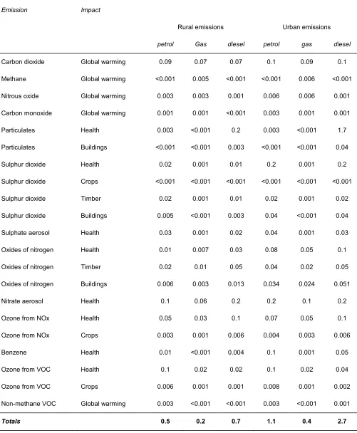
Eyre et al. (1997) used emissions-based dispersion modelling to estimate the exposure of the population of London specifically to road transport emissions and compared this with other impacts. Their results reproduced in Table 2 suggest that urban diesel particulate emissions have by far the most significant impact of all road transport emissions. Interestingly, the next most significant impact is secondary nitrate particles formed from emissions of NOx. The current European trend towards larger fractions of PM10 being composed of nitrate formed from NOx, much of which is of road
transport origin, is a trend towards the health effects of PM10 becoming increasingly an impact of road transport
emissions.
Sources of uncertainty and implications for transport
Despite the very large uncertainties in all valuations of impacts of air quality, the larger sums estimated in such studies have led to particulate air pollution causing at least as much concern over its effect on human health than any other ambient air pollutant world wide. The choice of PM10 as the measure of particulate air pollution to be controlled is based
on a biological plausibility argument given the aerodynamic characteristics of the human respiratory tract. The strength of the evidence for health effects of PM10 in general may be assessed against the criteria proposed by Bradford
Hill (1965), which are listed in Box 1. Much less certain is the extent to which primary PM10 from road transport exhaust
particulate emissions in Europe (the focus in the US is much more on regional secondary PM10 from large combustion
sources) must be described as precautionary.
If an estimate of population exposure used in an epidemiological study is subject to error, this will cause the observed relationship between air quality and health to be an underestimate of the true effect (Elwood, 1988). Critically, concentrations of pollutants from non road traffic sources tend to exhibit much less spatial variability than those from road networks, for example PM10 tends to be fairly constant over wide areas while NO2 can vary by an order of
magnitude over a hundred metres or so in a residential area close to a few major roads, such that it is much easier to assess exposure to PM10 accurately. This raises the prospect of PM10 appearing wrongly to be more strongly associated
with health effects than NO2, as discussed by Fairley (1990), on account of the effect of the road traffic related pollution
being diluted by exposure misclassification in certain designs of epidemiological study (Lipfert and Wyzga, 1995). The smallest diesel exhaust particles do not enter the human lung very easily because they undergo Brownian diffusion to the nose and throat, but the larger ones are close to the size that can penetrate the deepest into the alveolar regions of the lung where gas exchange with the blood occurs. Particles several micrometres in size from mechanical sources such as resuspension of road dust can dominate total PM10 mass but most of these are likely to be intercepted by
impaction in the nose. In recent years, toxicological laboratory studies predominantly carried out on rats has been driving interest towards smaller particles (for example, Peters et al. (1997), Ferin et al. (1991), Li et al. (1999)) and future legislation is currently expected to focus either on smaller particle mass fractions PM2.5, PM1, PM0.1 or on particle
number. This potentially has a very great impact on urban road traffic, especially if epidemiological studies can be designed to differentiate between the effects of diesel exhaust particles and the secondary acid sulphate and nitrate particles that are imported to an urban area from distant sources. The laboratory studies already show that particles from vehicle exhaust may not be the most toxic fine particles in the urban atmosphere, for example, quartz present in resuspended road dust appears to be much more toxic than diesel exhaust (Murphy et al., 1998), but if primary particulates from road traffic exhaust continue to be blamed for the observed health effects of PM10, precise details of
which particle sizes and composition are most important will determine which combination of fuel type, engine type and end-of-pipe emissions abatement technology is likely to be most effective at reducing impacts on human health. Such detailed information is currently unknown.
Finally, it must be noted that the chronic effect of particulate air pollution is potentially much larger and less socially acceptable than the acute, but is often omitted from attempts to quantify benefits of pollution control because estimates of the chronic effect are the most uncertain of all.
4.2. Impact of aircraft emissions in the upper troposphere and lower stratosphere on global atmospheric change
Factors determining magnitude of transport impact
The considerable visible and noise impact of large jet aircraft has resulted in their being considered frequently as potential significant sources of ground-level air pollution in the vicinity of major airports. Several studies (for example, ERL (1993)) have shown, however, that the emissions of the aircraft themselves contribute rather little compared with the great volumes of road traffic that large airports generate, plus other airport-related surface sources of air pollution. Even though an airport itself, typically located outside urban areas, can be the largest source of emissions in the vicinity, those from the aircraft themselves are efficiently dispersed before they reach the ground in the same way as the emissions from tall chimneys that were discussed in section 2. Future reductions in road traffic emissions and growth of the air transport industry may mean the aircraft contribution to ground-level air quality will become more significant relative to other sources, especially as pressure on land for expansion produces a tendency for increased airport development in cleaner air further away from the major cities that airports serve. Meanwhile, however, to find the most significant contribution of aviation to air pollution, we must look to higher altitude, where the lower atmospheric pressure and lack of other nearby anthropogenic sources of trace gases and particles means that a given volume of emissions can have a much greater impact.
Fig. 4 shows that hydrocarbons and carbon monoxide are emitted from jet aircraft engines predominantly on the ground. The major trace gas emission during flight is oxides of nitrogen (NOx). In addition, much larger quantities of carbon dioxide and water vapour are emitted, which illustrate some important issues of temporal evolution of emissions and impact for this rapidly expanding mode of transport. Furthermore, soot particles in the exhaust need to be considered for their roles as ice nuclei and in heterogeneous atmospheric chemistry.
The depends on how high the aircraft is flying. About half the NOx emissions from sub-sonic aircraft occur at the main cruising altitude of 10 to 12 km. Since the top of the free troposphere varies from about 8 km in polar regions to 16 km in the tropics, subsonic flight is in the lower stratosphere at high latitudes and in the troposphere elsewhere. On busy North Atlantic routes, as much as 75% of the total fuel per flight may be used in the stratosphere (RNMI, 1994). Supersonic aircraft cruise higher, always in the stratosphere, but at the time of writing the tragic crash of the Air France Concorde seems to be indicating that civilian supersonic flight is unlikely to return to our skies for several years at least.
In the free troposphere, emissions of NOx lead to the formation of ozone (Clemitshaw et al., 2000). This O3 can be
mixed down to ground level and contribute to regionally poor air quality during photochemical air pollution episodes in what is gradually becoming a global air pollution problem, and it is also a greenhouse gas. Formation of O3 by NOx is
reduced, however, by the way NOx leads to increased levels of photochemical oxidants and hence shorter atmospheric life-time of methane.
In the stratosphere, the chemistry of ozone is totally different. At middle and low latitudes NOx is involved in catalytic cycles that destroy the protective ozone layer in the stratosphere (reference to Millennium Review on the stratosphere) and can allow dangerous ultra violet radiation from the sun to reach the surface of the Earth. Even though emissions of sulphur dioxide and soot particles from aircraft are negligible compared with total global emissions, their potential to damage the atmosphere is even more enhanced in the stratosphere relative to at the surface than is the case for NOx. Sulphur dioxide in the stratosphere becomes oxidised to form droplets of sulphuric acid, and these with soot particles from aircraft exhaust promote heterogeneous chemical reaction cycles that destroy O3. These stratospheric clouds also
promote the conversion of NOx to nitric acid (HNO3), thus lessening the potential of the NOx to destroy O3 by gas-phase
chemical reactions, but at very low temperatures the HNO3itself can form droplets with then add to the heterogeneous
chemistry that destroys O3. Depletion of stratospheric ozone has a cooling effect on climate, partially offsetting the
warming effect of NOx from aircraft in the troposphere.
In comparison to these two indirect impacts of aircraft emissions on global atmospheric chemistry, the direct effect of CO2 from aircraft causing climate warming due to the ability of CO2 to absorb outgoing infra-red radiation is conceptually
simple. When comparing different impacts of aircraft upon the global atmosphere with each other, and with the effect of emissions from other transport sectors and non transport related activity, the most challenging aspect of CO2 is perhaps
the time scale over which it has an effect. CO2 is chemically sufficiently unreactive for its dominant removal process to
be physical. Solution in the water of the upper ocean and exchange of carbon between the atmosphere and terrestrial biomass are relatively rapid, with the combined annual flux amounting to 20% of the atmospheric carbon reservoir mass of 750 GT (Houghton et al., 1996), but these fluxes are bi-directional. The rate determining step for net removal of carbon is mixing from the surface and intermediate ocean to the much larger carbon reservoir of the deep oceans. At the turn of the 21st Century, anthropogenic carbon emissions of 7 to 8 GT per year (including deforestation) are greater than the equilibrium rate of removal at current atmospheric and surface ocean concentrations, such that an amount of carbon equal to around half the emissions each year are removed and the imbalance results in a steady increase in atmospheric carbon dioxide levels. Were emissions to remain constant at today’s rate, the atmospheric concentration would reach an equilibrium level about one third higher than today’s value towards the end of the 21st Century. The global total emissions of CO2 from aviation in 1990 was about 450 million tonnes of carbon (Barrett, 1991), which was
less than 20% of global road transport emissions and about 3% of total anthropogenic emissions. Furthermore, historical emissions of CO2 from aviation are almost zero going back just a few decades into the mid 20th Century, while
around half the carbon dioxide from all anthropogenic sources currently in the atmosphere was emitted before 1980, so the overwhelming majority of the total is from non-aviation sources. The small contribution of aviation is, however, increasing, and the small amounts of CO2 being emitted by aircraft now will remain in the air for many decades.
Finally, water vapour from jet engines can also form line-shaped clouds in the free troposphere. The temperature of these clouds is lower than that of Earth’s surface, so their black body radiation is less than what would be emitted from Earth’s surface were the clouds not there, resulting in net warming. This is more significant than the amount of incoming solar radiation reflected, so that overall the contrails have a warming effect on climate at the surface. Usually, contrails evaporate again within minutes or even seconds such that their impact is negligible, but under certain meteorological conditions they can be sufficiently persistent a large part of the sky can become obscured continually along a major flight path until weather conditions change many hours or days later. In the stratosphere, contrails are never persistent because of the low ambient relative humidity there, although the water vapour from aircraft is not removed rapidly by precipitation as it is in the troposphere so has a small warming effect on climate because of its greenhouse gas properties.
Current ability to quantify impact and major sources of uncertainty
In theory, the impact of aircraft emissions on upper troposphere and lower stratosphere chemistry can be quantified using global models of circulation and chemistry (such as Johnson et al., 1999). However, despite the fact that the reaction mechanisms are now qualitatively understood, quantifying the impact of aircraft emissions remains elusive. There are two main reasons for this:
Firstly, the chemical reaction cycles are complex, as different gas-phase and heterogeneous pathways become more important at different temperatures. Small errors in the predicted mix of different pollutants can propagate via resulting errors in the relative rates of two or more competing reactions to end up with quite unrealistic simulated O3
concentrations. Not only must the chemical composition of the upper troposphere and stratosphere be simulated accurately, but rates of mixing between layers as well as chemistry determines the composition, the temperature needs to be known to determine where heterogeneous processes occur, and the temperature has a large influence on the mixing. The whole process of stratospheric O3 destruction in particular is a highly non-linear catastrophic process.
Secondly, emissions of aircraft in the upper troposphere and stratosphere occur along highly localised flight paths that vary in time and space. The physical size of these is much less than the resolution of the global-scale models that are required to simulate chemistry in the upper troposphere and stratosphere. This problem of scale is added to the fact that the total emissions from aircraft are at least as difficult to quantify as emissions for road traffic are on the ground. It is exacerbated by the fact that other sources of the same pollutants in the upper troposphere and lower stratosphere, such as lightening and mixing from the lower troposphere, are also very difficult to quantify accurately.
Any one of these difficulties would make calculations of the total atmospheric impact of aircraft emissions liable to error. Combined, they present a very formidable challenge indeed for the science of atmospheric chemistry modelling. The most recent calculations indicate that the effect of aircraft NOx emissions on producing O3 in the upper troposphere /
(Penner et al., 1999). The greatest overall expected change in O3 due to aircraft emissions is thus an increase of about
6% in the region 30 to 60°N at 9 to 13 km altitude. Observational evidence of this is very difficult to find, because O3
variability is high near the tropopause and the expected 20% increase in NOx due to aircraft emissions is substantially smaller than the observed variability. However, in presenting these results, the IPCC Working Groups stress that the models include some notable deficiencies in the physics and the gas-phase and heterogeneous chemistry of the problem. To reduce the uncertainties, a concerted effort is therefore required, combining model development with detailed field observation campaigns that recent instrument development and improvement have made possible. Quantification of the direct climate change impacts of aircraft through their CO2 emissions is arguably not so fraught with
difficulty. The global climate models that are now in an advanced state of development are, nevertheless, extremely complex. A discussion of these and uncertainties therein is beyond the scope of this review. The sub-grid size of contrails however presents some problems similar to those discussed for NOx chemistry, and the sensitivity of contrail persistence to meteorological parameters presents a test of model accuracy in regions where such performance requirements have not been demanded before and where validation data are sparse, on top of the effects of significant remaining uncertainty surrounding ice nucleation processes.
A significant area of debate is concerned not so much with the accuracy of our predictions about the impact of aviation on climate, but with how to respond to the implications. In terms of the size of the perturbation to the radiation balance, the latest calculations are sufficiently accurate to indicate that contrails have at least as large an impact on climate as CO2 emissions from aviation, and that the radiative forcing due to contrails could be several times larger if less
conservative estimates of the more uncertain contrails impact are used. If the formation of persistent contrails could be prevented, however, the radiation balance of the atmosphere would respond immediately, in contrast to CO2 from
aviation in the 20th Century which will remain in the atmosphere for several decades. Integrated over a long future time horizon, CO2 emissions thus may be considered the most significant impact of aviation on the global atmosphere. Faced
with a choice between preventing contrails or reducing overall fuel consumption, the decision must therefore be whether we want to make a small contribution to the solution of a long term problem but possibly severe problem or if a larger, instantaneous benefit is sufficiently desirable to be worth paying for in the latter part of the century.
In contrast to the human health effects of urban air pollution, where economic valuation was attempted at least for the acute effects, assessment of the implications of global atmospheric change are mostly qualitative. A most comprehensive example of this is Watson, Zinyowera and Moss (1996), which catalogues a wide range of impacts of climate change, but does not attempt to judge whether or not these impacts constitute “dangerous anthropogenic interference with the climate system” on the grounds that definition of what is “dangerous” is a political not a scientific judgement. For the impact of stratospheric ozone depletion on human health, which is expected to result in increased incidence of skin cancer over several decades, the magnitude of the effect is very difficult to quantify, for similar reasons to the difficulty in quantifying chronic effects of urban air pollution on human health.
4.3. Controlling acidification: sulphur emissions from ships
Factors determining magnitude of transport impact
The acidity of the polluted atmosphere is enhanced relative to the clean atmosphere by the oxidation of oxides of sulphur and nitrogen. As has already been discussed briefly in section 3, catastrophic damage to upland forests attributable to acid deposition led to land-based European emissions of sulphur being reduced by 40% between 1980 and 1993 (Barrett and Seland, 1995). These emissions are principally from large coal-fired combustion plant, and reductions have been achieved by changing to a fuel with a lower sulphur content (including natural gas) or fitting flue-gas desulphurization abatement technology. At the time of writing, the Second Sulphur Protocol (UNECE, 1994) has been ratified by 22 of the 28 parties. Meanwhile emissions of NOx have remained almost constant, as have emissions of ammonia (although the estimates of ammonia emissions are subject to large uncertainties). This means that nitrogen is now more significant than it has been in the past, and the major ground-level transport source of oxides of nitrogen is road traffic. Pressure to reduce acidification further therefore enhances the focus on road traffic as a major source of air pollution that was discussed at length with respect to particulates and health in Section 4.1. Shipping, however, remains a transport source of sulphur that has not been subject to the abatement measures applied to sources on land, albeit a much smaller contribution to atmospheric acidity than oxides of nitrogen from road traffic. The argument that these emissions from marine transport should also be reduced will therefore be based on calculations of the costs and benefits associated with such measures.