Journal of Fluid Mechanics
http://journals.cambridge.org/FLMAdditional services for Journal of Fluid Mechanics:
Email alerts: Click here Subscriptions: Click here Commercial reprints: Click here Terms of use : Click here
Theory and computations for breakup of unsteady
subsonic or supersonic separating flows
I. P. Vickers and F. T. Smith
Journal of Fluid Mechanics / Volume 268 / June 1994, pp 147 173 DOI: 10.1017/S0022112094001308, Published online: 26 April 2006
Link to this article: http://journals.cambridge.org/abstract_S0022112094001308 How to cite this article:
I. P. Vickers and F. T. Smith (1994). Theory and computations for breakup of unsteady subsonic or supersonic separating flows. Journal of Fluid Mechanics, 268, pp 147173 doi:10.1017/ S0022112094001308
Request Permissions : Click here
J . Fluid Mech. (1994), vol. 268, pp. 147-1 73
Copyright 0 1994 Cambridge University Press
147
Theory and computations for breakup of unsteady
subsonic or supersonic separating
flows
By
I.
P. VICKERS A N D F.T.
SMITHMathematics Department, University College London, Gower Street, London WClE 6BT, UK
(Received 6 July 1993 and in revised form 13 November 1993)
This study of flow just beyond a breakaway-separation point presents a description of planar nonlinear unsteady effects over a fairly wide parameter range, for a subsonic or supersonic boundary layer at large Reynolds numbers. The inviscid model thus produced essentially contains a vortex sheet near the smooth solid surface, with local inner-outer interaction. The governing equations couple the eddy velocity and pressure with the thicknesses of the detached boundary layer and the eddy. The computational method presented here uses a new adaptive gridding technique intended to capture accurately the spiky solution behaviour that develops and to compare with theory. Analysis and computations point to a breakup in the solution, suggesting an explanation for the start of transition and possible turbulent reattachment as found experimentally. The influence of the detached boundary-layer thickness proves crucial. The type of finite-time breakup encountered is studied analytically and the criterion for its occurrence is highlighted. This is guided by a characteristic analysis for a special case. The finite-time breakup is similar in spirit to, although different in detail from, a nonlinear breakup proposed earlier by one of the authors for general unsteady interactive boundary layers and it suggests a wide application of that nonlinear breakup theory and its criterion. Comparisons between computations and theory are found to be supportive.
1. Introduction
There are three chief points to this paper. The first is to present an account of nonlinear unsteady effects on separating flow in a certain fairly wide parameter range, for an incompressible or compressible boundary layer. The model thus produced, containing a vortex sheet near the solid surface, leads to breakdown in the solution and suggests an explanation for the start of transition and possible turbulent reattachment as observed experimentally. In particular the influence of the local shear-layer thickness proves crucial. Secondly, a numerical method is to be described which uses an adaptive gridding technique aiming to capture accurately the spiky solution behaviour that develops and to compare with theory. The third point is to study analytically the type of finite-time breakup encountered in the solution, and the criterion for its occurrence. This is similar in spirit to, although different in detail from, a nonlinear breakup proposed (Smith 1988) for other contexts and it suggests a wide application of that nonlinear breakup theory and its criterion.
148 I. P. Vickers and F. T.
Smith
laminar separation upstream, followed by turbulent reattachment downstream, is often found in practice and in various computations, as in Burmall& Loftin (1951), Gault (1955), Tani (1964), Gaster (1966), Mehta (1977), Mueller & Batill (1980), Van Dyke (1982), Young (1982), Vatsa & Carter (1983), Mueller (1984), Dovgal, Kozlov &
Simonov (1987), Kozlov (1987), Mezaris et al. (1987). Concerning computations, the flow solution depends crucially on the position of laminar-turbulent transition and hence on the transition criterion used, which is often based on empiricism. Much of the literature is reviewed by Smith & Elliott (1985), who also provide a theoretical account based on unsteady marginal separation which reproduces some of the observed features. Alternative paths to stall or transition involving some unsteady separation are studied by Peridier, Smith & Walker (1991 a, b), Hoyle, Smith & Walker (1991), Smith
& Bowles (1992), Smith (1993). Our concern likewise is with unsteady separation and transition, taking two-dimensional flow as a starting point but with less restrictive assumptions than in Smith & Elliott (1985) on the underlying separation motion. Indeed, the starting separating motion assumed here is believed to be in its most general form (Stewartson & Williams 1969, 1973 for the supersonic range; Sychev 1972, Smith 1977 for the incompressible or subsonic range). It is then found below that both small-scale and large-scale separations are very prone to linear and nonlinear instability and subsequent transition, as in practice, and especially so for the large-scale forms, and the nonlinear breakup criterion mentioned in the previous paragraph applies here.
The underlying, starting, flow is governed by the triple-deck solution of the last two named references, in the incompressible case which we address mostly in this section. The solution compares favourably with experiments, as shown in Fiddes (1980), Smith (19863) for instance, for large-scale breakaway separations: see also the reviews by Messiter (1983), Stewartson (198l), Smith (1982), Sychev (1982). In the triple-deck local interaction a sizeable adverse pressure gradient, with only a small pressure rise, leads to regular separation of the boundary layer, avoiding the Goldstein singularity. Two kinds of separation may be identified: small-scale separation, near a small deformation such as a slight change in the surface conditions compatible with the interactive scalings (see reviews above) ; and large-scale separation, provoked by a sizable disturbance, say an obstacle of finite dimensions, or on a bluff body. Our concern is mostly with the second kind. There the majority of the oncoming boundary layer is shifted away from the body surface and eventually appears within the outer flow downstream as a thin free shear layer of concentrated vorticity, separating regions of predominantly inviscid flow, if the steady state persists. The shear-layer thickness then is typically O(Re-iZ*), where
I*
is the global lengthscale.Breakup of unsteady subsonic or supersonic separating Bows 149 including inflexional velocity profiles, while the local curvature of the separating flow can provoke Gortler instabilities also. Linear instability properties are clearly of limited relevance to the practical configurations described earlier, however, because in practice the mean flow is substantially altered from the laminar form during stall and transition, and so our emphasis here moves on to nonlinear properties; likewise three- dimensional effects and other parameter regimes, e.g. as in Brown, Cheng & Smith (1988), require further study.
Nonlinear unsteady effects are clearly necessary to account for the transition and stall in the separating flows of current interest. Little seems known as yet on the influence of such effects, but the unsteady nonlinear triple-deck system provides a most appropriate starting point. We then focus on relatively fast scales equivalent to the so- called high-frequency regime (Smith & Burggraf 1985; Zhuk & Ryzhov 1982; Smith, Doorly & Rothmayer 1990) and corresponding to increased distances downstream. The major flow properties there are inviscid, subject to assumptions about thin viscous layers which are discussed later. The same evolution equations result, in fact, if the Euler equations are taken as the starting point. Moreover, significant effects due to the thickness of the separated shear layer can be incorporated in the near-surface motion, cf. Moore (1979), Saffman & Schatzman (1982a, b). This aspect is presented in 92 for large-scale two-dimensional separations, based partly on the suggestions in Smith (1987). The high-frequency parameter used is Q($ l), which is related to the scaled distance downstream of separation being large in triple-deck terms, cf. (1.2) below, and to the range of dimensional frequencies Q*, contained within the nonlinear disturbances, defined by
where U * is the global velocity scale. The corresponding streamwise distance
x*
beyond separation is in the rangeRe;
<
Q*l*/U* 4 Ref, (1.1)Re-;
<
x*/l*<
Re-&. (1.2) Given (l.l), (1.2), the nonlinear evolution equations of $2 then hold for the unsteady separated eddy velocity, the surface pressure, the eddy thickness and the change in boundary-layer thickness, in scaled terms. The range (1. l), (1.2) controls ' mid-scale separation', and it includes thickness effects that contrast with Brown et al.'s (1988) model which applies instead for global-scale separations effectively. The shear-layer thickness present in mid-scale separation smooths out the terminal solution behaviour found by Brown et al., as Vickers (1993) shows, and instead another type of terminal behaviour emerges (93). This is akin to the finite-time breakup of Smith (1988) and is considered in detail in g3, including the criterion for breakup.150 I. P. Vickers and F. T. Smith
for the Burgers equations, as described in Vickers (1993), and it is used in
$4
to check the analytical suggestions of9
3 and test the breakup criterion.Further comments are provided in $5. The Cartesian coordinates x, y, the corresponding velocity components u, ZI and the pressure p used are non-dimensional, with respect to the typical global lengthscale I* (e.g. the airfoil chord), to the velocity scale U* (e.g. the local main-stream speed) and to p*U*’, where p* is the fluid density. The time t is non-dimensionalized with respect to l*/U*, while Re
=
U*Z*/v* is large,v* being the kinematic viscosity of the fluid. Supersonic motion is also considered below, in B22-4. The solid surface is taken to be flat locally, given by y = 0, with the original laminar separation taking place at x = 0, followed by nonlinear unsteady interaction occurring downstream focused around an x-station lying within the range of (1.2).
2. Nonlinear disturbances in separating flow
The breeding ground for all the separating flow instabilities can be regarded as the triple-deck structure, in two or three-dimensional form, as we shall see; this structure describes not only initial TS waves but also the first appearance of inflexional modes (Smith 1987 and below) and it connects up with Gortler instabilities via its three- dimensional characteristics. It is important, in addition, that the triple-deck structure also governs the basic, separating, flow (Sychev 1972; Smith 1977) locally, which is an unfortunate point in a way, as the linearized instability problem for such a basic flow is then found to be almost irretrievably non-parallel in nature. In scaled terms, with h
denoting the local skin-friction factor and (figure 1)
( x , ~ , z, t) = (2-k3x, A-@Y, h-tE32, A-QT), (2.1 a)
(U,Y, w,p) = ( h i d , &3v, &W, hb’P), (2.1 b) where E E Re-&, both the separating flow and its major instabilities are therefore controlled by the nonlinear viscous-inviscid interactive problem
with
au
av
-+-
= 0,ax
a yau au au
ap a 2u
-+
u-+
v-
=--(I,
T)+-8~
ax
ayax
ay2’U = V = O at Y=O, U - Y+A(X,T) as Y + m ,
(2.24
(2.2 b)
(2.24 (2.2d)
(2.2e)
where denotes the principal value of the Cauchy-Hilbert integral and we restrict ourselves to two-dimensional features. Here (2.2~-d) hold in the lower deck. The basic steady separation is present for 2/aT identically zero, with the unknown displacement increment - A = - drising as X i far downstream for an open or breakaway separation
Breakup of unsteady subsonic or supersonic separating flows
(4
...
.
....
...>..~...~...~...*.... ...... *..
...
---3x
151
Inviscid
/
.c-
Inviscid
... ... - +
t;":
...-
t
-.
viscous- - -
...
...
-x
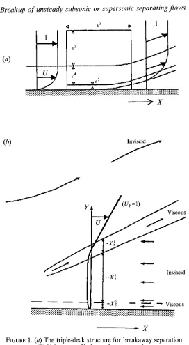
FIGURE 1. (a) The triple-deck structure for breakaway separation.
(b) Velocity profile beyond the separation.
instabilities. For, if a small unsteady disturbance (decomposed as exp (iaX-iQT)) of scaled frequency Q is made in the incoming motion upstream, i.e. where the basic motion is the parallel one
U
= Y,V
=W
= P =A
=
0, then the disturbance becomesunstable (Smith 1979, 1 9 8 6 ~ ; Zhuk & Ryzhov 1980) for
where 0, M 2.30. This linear instability of the parallel attached flow is none other than the TS instability, governed by the linearized unsteady version of (2.2). The nonlinear unsteady version then yields nonlinear TS waves (Smith & Stewart 1987a; Smith 1984,
1986 a ; Duck 1985), travelling unsteady separations (Conlisk, Burggraf & Smith 1987)
152
I. P.
Vickers and F. T. Smithand the possibility of breakup (Smith 1988; Peridier et al. 1991 a, b ; Hoyle et al. 1991) and transition downstream. Separating basic motion, by contrast, in general poses a more difficult nun-parallel-flow problem as regards the instability since the lengthscales of the separating motion and the instability coincide, which is an unfortunate point rendering the above decomposition invalid. That is, the governing equations for a small disturbance generally cannot be reduced from partial- to ordinary-differential ones, in the conventional Orr-Sommerfeld fashion, because the coefficients U, are non-trivially dependent on
X,
Y in separating flow. Unfortunately, this somewhat obvious point is overlooked in some studies of separating-flow stability.The main options available therefore are: a computational treatment of the linear or nonlinear partial-differential equations (2.2) or their three-dimensional counterparts, for an initial-value problem say (which is likely to lzad to the finite-time breakup of Smith 1988, see Peridier et al. 1991a, b ; Hoyle et al. 1991); or an analysis based on relatively short-scale properties (where linearly the streamwise variation of U,
V
during separation is a secondary effect). We pursue the latter course for incoming TS-like waves upstream, to find how they might develop and change as the flow separates. See also Smith & Bodonyi (1985), Tutty & Cowley (1987) as regards inflexional instability, again within shorter lengthscales. Linear short-scale TS waves corresponding to large values ofB
are found to remain neutral at leading order, with the amplitude growth or decay being fixed at higher order by a combination of viscous and non-parallel-flow effects (Smith 1986a, 1987; Smith & Stewart 1987b), the spatial growth rate G coming(2.4)
out to be
Hence an increasing/decreasing basic displacement ( -
x)
has a destabilizing/ stabilizing effect on the incoming waves, as would be expected physically. For breakaway separating motion in particular the growth rate increases indefinitely downstream, on the present scale, since-KO=
X i then (Smith 1977) (see figure 1).Hence a new phase is entered relatively far beyond the separation point. On linear or nonlinear grounds the critical distance Xcrit = L involved is
O(Bi),
where the main short waves have length O(L-g) locally and the scaled departure distance is Lbf, say, where d is O(1). These scalings follow from (2.4) or from an order-of-magnitude argument as in Vickers (1993), Smith (1987). At the O(L) distance beyond separation the unsteady-flow behaviour revolves initially around the stability of a simple quasi- parallel basic flow (figure l), namely the uniform shear0
-
Y - A above the now- detached shear layer, for Y>
A, and the negligible flow 101<
1 underneath, for0
<
Y<
A , in scaled terms. This base state is the far-downstream form of the steady breakaway-separating motion in Smith (1977). The associated linear and nonlinear stability properties are predominantly inviscid, or rather, in the nonlinear regime, will be taken to be so at the first approximation.G = 1/(22/2)+$(-dA/dX).
The nonlinear equations of concern stem from (2.2), with
(U,
v,
P , A ) = O(Li, Li, L3, L:) (2.5)and X-+L+L-aX, Y+ Lg Y henceforth. The detached shear layer now takes an unknown shape LZS, where we note again the abrupt O(L-f) X-scale. The governing equations above and below the thin shear layer or interface are therefore the inviscid virsions of (2.2),
au
av
-+-
= 0,2x
2Y ( 2 . 6 ~ )au
au au
apaT
ax
ayax,
Breakup of unsteady subsonic or supersonic separating flows 153 subject to V = 0 at Y = 0, U
-
Y + A(X, T ) as Y-tco
as before but now the kinematic constraint at the interface requiresas
as
V =
-+
U - at Y = S(X, T ) + ,aT
ax
(2.6~)Here T+LP3T. Also, a simple assumption of tangential flow is made at the solid surface, although that is likely to prove invalid at later times (see also Smith & Burggraf 1985; Smith 1987, 1988; Peridier et al. 1991a, b). If zero vorticity is present initially below the shear layer then the solution of (2.6~-c) there produces
(2.7)
au
u =
U ( X , T ) ,v=-Y-
ax’
so that
as
a(su)
-+-
aTax
= 0.(2.8,)
(2.8 b)
Above the shear layer, by contrast, there is non-zero uniform vorticity such that
from (2.6a, b) and so (2.6~) yields
a
a
ap- ( S + A ) + ( S + A ) - ( S + A ) = --
aT
ax
ax‘
(2.104The nonlinear system controlling U , P , S , A in this case is closed by the pressure- displacement law
(2.10 b)
in view of (2.2e). Linearized features provide some useful guidelines and checks. As a check the linearized version of (2.8a, b) and (2.10a, b), for a small disturbance about the exact uniform state U
=
0,P
E 0, S=
A , A E - A , reproduces the dispersion relationa3d - 01252
+
Q2 = 0for wavenumber a, frequency 52, as in Smith (1987). This relation has certain notable properties. First, it provides a continuation from the incoming attached-flow TS mode upstream, since there d --f 0 and the second and third terms in (2.11) then dominate,
giving a+52$ as in Smith & Burggraf (1985), Smith (1986a, b). Secondly, inviscid inflexional Rayleigh-type waves are possible also, these occurring when interaction is suppressed (the A-disturbance --f 0) and the first two terms in (2.11) become dominant,
154
I.
P.
Vickers and F. T. SmithFIGURE 2. Illustrating the effect of the eddy velocity U, on instability via the left-hand side of
(2.15). The case (2.11) corresponds to U, = 0.
significant feature, is the criterion for instability, i.e. complex roots for a from (2.1 1). For real wavenumbers a the relation (2.9) always yields temporal instability provided d > 0, but for the practical alternative of a fixed-frequency disturbance, with
O
specified as real, (2.9) is found to yield spatial instability if d exceeds the value where (see figure 2)&it = 3(9 2 1 0 :
1
. (2.12~)But since d = ($b)Xg to leading order, with b zz 0.44 (Smith 1977, and see Korolev 1980), this yields the prediction
Xcrit = (O/3b2)i (2.12 b)
for the distance between the separation point and the position of abrupt enhanced instability. In dimensional terms, (2.12 b) becomes
x:Tit = l*(a*l*/3b2U*)Jh-~Re-~ (2.13)
from use of (2. l), where 52" is the dimensional frequency imposed. The range of validity of (2.13) is restricted, however, to
Re: V / l *
4
O* 4
Re; U*/I*, (2.14) the left restriction ensuring that the scaled frequencySZ
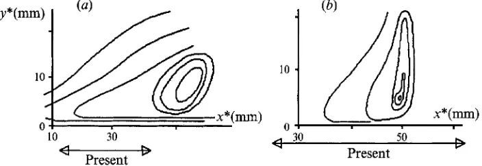
is large and the right restriction requiring the detachment distance to remain small compared with the detached boundary-layer thickness. Comparisons of Mezaris et al.'s (1987) experimental results and the prediction (2.13) show an encouraging amount of qualitative agreement, and possibly also quantitative depending on the precise value of the skin-fraction factor A,as shown in figure 3.
The relation (2.1 1) suggests something more, however, namely the existence of a threshold amplitude for the nonlinear growth of disturbances, because of (2.12~). That is, nonlinear disturbances may grow (if d locally exceeds dcrit) in the interval upstream of the linear growth point of (2.12b) or (2.13), thus causing substantial instability to arise sooner. We note in passing that an upstream movement of Xcrit, corresponding to reduction of dcrit, also results if there is significant reversed flow present in the eddy, since linearization about U = U, and S = - A = d changes (2.11) to
a3AL'+(SZ-aUo)2(52-~2) = 0. (2.15)
Thus if U,
<
0 complex roots for 01 arise at smaller values of d than for (2.1 l), i.e.Breakup of unsteady subsonic or supersonic separating flows 155
10 30
Present
50
Present 3
FIGURE 3. Comparisons with the experiments of Mezaris et al. (1987), showing disturbance amplitude contours at (a) 0.2 Hz, (6) 0.5 Hz. The present prediction (2.11) of length is shown arrowed in each case.
Henceforth we consider the governing equations (2.8a. b), (2.10a, b) and their
P =
-a~/ax.
(2.16)Equations (2.2a-d) with (2.16) (and hence (2.8a, b), (2.10a), (2.16)) are obtained via a transformation analogous to (2. l ) , but the orders of magnitude corresponding to
(2.5) are different as
- A
cc X far downstream for supersonic breakaway-separating motion (Stewartson & Williams 1969, 1973). We note also that the supersonic-flow analogue of much of the above analysis goes through with (2.16) replacing (2.2e), (2.10 b) and hence (2.1 1 ) being replaced byu3A - a252
+
i 0 2 = 0, (2.17) which yields linear spatial instability for all d>
0. Thus it is interesting that separation immediately destabilizes supersonic motion, even though attached supersonic motion is stable to the original viscous-inviscid waves.Finally here, we note the effect of the relative thickness of the separated boundary layer, which is implicit in the governing equations (2.8a, b), (2.10a, b), (2.16), cf. Kachanov, Ryzhov & Smith (1993) in attached flow. The right-hand restriction (2.14),
in requiring the detachment distance to remain small compared with the detached boundary-layer thickness, maintains the triple-deck balance and hence our starting point is the system (2.2a-e), for a subsonic main-stream flow. However, the current configuration is sufficiently far downstream of the separation point for the flow field to be decomposed into two regions of predominantly inviscid motion separated by a thin shear layer or interface, and a viscous wall layer. The flow in the wall layer is governed by the viscous unsteady boundary-layer equations driven by the pressure gradient determined from the inviscid flow above. Hence this layer remains passive with respect to the main inviscid flow regions above or is assumed to be so (see below, however). The displacement across the boundary layer, in contrast, requires matching with the outer inviscid motion (in the major part of the boundary layer) and results in the flow forms after (2.8b), which in turn yields the equation (2.10a) controlling the expression S + A . This expression, i.e. the difference between the scaled shear-layer shape S and the scaled boundary-layer displacement - A , is therefore representative of the effect of the flow within the detached boundary layer. That is to say, although the shear layer is taken to be relatively thin, the overall boundary-layer thickness. nevertheless exerts an influence on the main flow field.
156 I. P . Vickers and F. T. Smith
3.
The
finite-timebreak-up
The possibility of a finite-time breakup of the mid-scale system (2.8a, b) and (2.104b) or (2.16) is considered here. This is partly in the light of the results of the numerical study in $4 below and partly due to Vickers' (1993) findings concerning the Brown et al. (1988) singularity as mentioned in $ 1.
3.1. A reduced system
In preliminary numerical trials for (2.8a, b) (2.10u), (2.16) starting with smooth initial conditions at time T = 0, the scaled streamwise velocity U and eddy width S appeared to develop quite severe behaviour near a particular X , T
>
0, with sharp changes in the slopes there: see Vickers (1993). Moreover, the variation of the scaled boundary-layer displacement -A rapidly decayed to zero across much of the domain. This phenomenon was little affected by grid-structure effects. The decay of A-variations to zero compared with the behaviour of U, S prompts us to consider in this subsection the limiting case of the variation of A being negligible throughout. In this case we discount terms involving A and its derivatives from the left-hand side of (2.10a) at leading order. The only contribution from A is to couple the behaviour of U, S via the pressure gradient (and (2.10b) or (2.16)) on the right-hand sides of ( 2 . 8 ~ ~ ) (2.10~).We then arrive at the following, smaller, homogeneous system controlling U, S :
(3.1 a)
(3.1 b)
which can be solved exactly. The solution can be expressed in terms of the Riemann invariants,
dX d T
r --Su+XS2-1
,
,[S(4U--3S)]; on - = U+$S'+~[S(4U-3S)]~, (3.2u, b)1 -
these being constant along their respective characteristic curves (3.2 b), (3.3 b) in the ( X , T)-plane, for some range 0
<
T<
say.The analytical solution (3.2), (3.3) is prone to break down, however, which can be seen from (3.2b) if the expression S(4U- 3 s ) (= D, say) takes negative values. As long as D remains positive the solution (3.2a), (3.3a) remains unique and well-behaved. However, if D approaches zero there is the possibility of the characteristics from (3.2b), (3.3b) intersecting in the
(X,
T)-plane but with rl =+ r2 in general. Hence the solution becomes multivalued there. So the system (3.1) tends to break down in the neighbourhood of a point(X8,
q),
say, with D --f 0+
as T+ T, - 0.Locally, near the first intersection of characteristics the relevant coordinate is
6,
defined byBreakup of unsteady subsonic or supersonic separating flows 157
unsteady-nonlinear balance of terms in the neighbourhood (3.4), the expansion
U
-
U,(O+
(T, - T)"-'U1(g)+
. . .
is examined as a candidate, and similarly for S. This leads to a contradiction, however, as Vickers (1993) shows. The corrected expansions, from an order-of-magnitude analysis of the characteristic curves, are (U, S )-
(u,,
So)(8
+
(T, - T)"(U,, S,)(g)
where m>
0. Then the left-hand side of (3.2b)or (3.3b) is of the form O(l)+O(T,-T)"-l, while the right-hand side is O(1)+
O(T, - T)"
+
O(T, - T)"'', as the term in the square root is zero at leading order. Matching terms implies thatin contrast with the first guess above.
Having established this corrected scaling we could proceed with the analytical solution of the reduced system (3.1 a, b) but instead we return to the full mid-scale system (2.8a, b) and (2.10a, b) or (2.16), for which (3.1)-(3.5) is very suggestive.
m = 2(n- I), (3.5)
3.2. The mid-scale breakup governing equations
An exact solution as in 63.1 seems unavailable for (2.8~1, b) and (2.10a, b) or (2.16). But the breakdown behaviour for the latter is postulated to be similar, dominated by the nonlinear interaction of U with S, and the breakdown in 93.1 for smooth initial conditions suggests the following typical collapse for the full mid-scale system
(2.8a, b) and (2.10a, b) or (2.16). It is focused around a station X = X,, at time T = T,, with
[U, SI
-
w,,
Sol(9
+
(T, -,>-
[Ul,
Sll(8
+
(T, -w z ,
S,l(8
+(T, - T)4n-4 [U,, S,] (8
+
. . .,
(3.6a, b) A N A,+(T,- T ) 3 n - 2 A 1 ( ~ + ( T , - T)4n-3A2(Q+((T,- T)5"-4A3(Q+ ....
( 3 . 6 ~ )Here f;, defined as in (3.4), is O(l), while A,, C, are constants. The constant n
>
1 is to be determined. The expansion ( 3 . 6 ~ ) is such that the only leading-order contribution from A , apart from the constant coefficient A,, is via the right-hand sides of (2.8a),( 2 . 1 0 ~ ) . The description (3.6a-c) might seem incomplete at first sight, as one might expect an O(T,- T)n term to be presented in ( 3 . 6 ~ ) to balance with the leading-order terms below. However, as is verified below, the inclusion of such a term would violate the hierarchy assumed above.
On substitution into (2.8~1, b), ( 2 . 1 0 ~ ) (2.16) we find at leading order, O(T,- T)-",
that U,, S, take constant values. Secondly, at O(T,- T)-', we obtain n[U; = n&S'h = 0, which again are satisfied identically by the constant solutions U,, So. The next set of successive equations, at O(T, - T)n-2, is
(U,-C,)
u;
= A;, (u,-c,)S;+S,u;
= 0, ( S , + A , - C , ) S ; = A;. (3.7a-c)We may eliminate A, from (3.7a, c) to see that ( 3 . 7 ~ - c) control U,, S,, with A , then determined from these. However, for a non-trivial solution of (3.7~-c) the constants L7,, So, A , must satisfy the identity
(Uo-C,)2+SO(SO+Ao-Co) = 0, (3.8)
with the result that
U,,
S, remain undetermined at this order. Equation (3.8) is none other than the characteristic equation, as above, thus confirming the relevance of the reduced system studied in $3.1.The unique solution for C, yields
4(U0-A,)-3S, = 0, 2 ( u 0 - c 0 ) + S 0 = 0. (3.9a, b)
158
So, since S, defines the local eddy width, S,
>
0 and U,, - C,,<
0 to satisfy (3.9b). These two conditions and the criteria (3.9a, b) help to simplify the final governing equations below.We must appeal to higher-order terms, therefore, with the O(T, - T)'%-' equations being found to be
( 3 . 1 0 ~ ) (3.10b) (S,+A,-Co)S;+n~S;-(2n-2)Sl = A;, ( 3 . 1 0 ~ )
I. P. Vickers and F. T. Smith
(U,-C,) u;+n@;-(2n-2)
u,
= A;, (U,- C,)s;+n&s;
-(2n-2) S ,+so
u;
= 0,and finally at O(
T,
- T)3n-4 we have(U,-C,) U;+n<U;-(3n-3) U 2 + U , U ; = A:, (3.11a) (U,-CC,)S~fn~S',-(3n-3)S,+S, u;+(S,
u,>,
= 0, (3.11b) (S, + A , -C,,)
S ;+
n[S; - (3n - 3) S, -I- S, S ; = A;. ( 3 . 1 1 ~ )Here the supersonic case (2.80, b), (2.10a), (2.16) has been chosen, but the subsonic case (2.8~1, b), (2.10a, 6) involves little change. As we shall see below, the above equations provide the final governing equations for the leading terms U,, S,, with A , then following from (3.7a-c).
Naturally, we tackle (3.10) first and use (3.8), (3.9) to eliminate U,, giving
nLJ2U;-S;)-(2n-2)(2U1-S1) = 0. Then the integral of (3.7b) in the form
S, - 2U, = d, where d is a constant of integration, requires that (2n - 2) d = 0. Hence
d = 0, since n
>
1, ands,
= 2u1, (3.12)although we have yet to discover the governing differential equation.
We obtain this equation finally from the reduction of (3.11 a-c). As before we make use of (3.8), (3.9) to eliminate U,, S,, giving on differentiation
nt(2U;- Sg) - (2n - 3) (2U; - S ; )
+
(U!+
S, U, - Sf)" = 0. (3.13)Then the combination of (3.12), (3.9a, b) with (3.10b) and its derivative eliminates U,,
S, from (3.13), to yield
{ - n z [ 2 + ( U , - C , ) U,) U ~ - { T Z ( ~ ~ - ~ ) [ + ( U , - C , ) U;> U/,-(2n-2)(2n-3) U, = 0. (3.14)
as the equation controlling U,, with S , then given by (3.12).
The permitted values for n are still not precisely determined although the supposition, implicit in (3.1 1 c), that the A-dependence on the left-hand side of (2.10a) remains negligible adds the upper limit n
<
2, so that n must lie in the range1 < n < 2 .
This result is due to (3.11a-c) being found at O(T,-T)3"-4, while the leading contribution from A is O(T,- T)'%-,. If, on the other hand, an O(T, - T ) % term were
included in ( 3 . 6 ~ ) the above reasoning would require n <
$.
The most likely value forn (see below), however, would violate this restriction and so, as stated above, this O(T, - T)" term is omitted from ( 3 . 6 ~ ) . In addition such a term in ( 3 . 6 ~ ) would yield a contribution much greater than those in (3.lOa,c), thus destroying the solution structure.
Ultimately, then, the present breakdown analysis reduces to the solution of (3.14).
This is a nonlinear second-order ordinary differential equation for U, as a function of the independent variable $ which varies from - co to
+
co. Ideally, we would hope forBreakup of unsteady subsonic or supersonic separating flows 159 Brotherton-Ratcliffe & Smith (1987), Smith (1988). However, attempts to find such an analytical solution were unsuccessful and instead we turn to an alternative approach in the following subsection.
3.3. Solution for the mid-scale breakup
Addressing (3.14), we scale out the negatiye constant (U, - C,,) with the transformation:
[ = -(U,-C,)[, U,(LJ =
-(u,,-c,,)~(~),
to arrive at(nzp
+ j ) y
+
{n(5 -3n)(+y>y
+
(2n -2) (2n- 319 = 0. (3.15) A prime now indicates differentiation with respect to[.
In the following, (3.15) is transformed to an equivalent autonomous first-order system, using the property that (3.15) is scale-invariant. The transformation hasj@) =
P Z ; < ~ ,
(
= eq (for[
>
0,(
<
01,
~ ( z i ) = li,, (3.16 a-c)whence (3.15) becomes
(3.17 a, b)
Applying a phase-plane analysis, we begin with the critical points (zi, 6) = (0, 0),
(- 1,O). The origin is a stable node, with
[h, 61
-
dl [n, - 21 exp (- 2q/n)+
d,[n, 31 exp (- 3q/n)locally, where d,, d2 are constants. Likewise it is found that the point (- 1,O) is a saddle, while from (3.17~) the trajectories must cross the li-axis with an infinite slope and from (3.17 b) they must cross the curve
6 = - 1 2(7
+
5n) T [(Sli+
7n-y)2
- 24(n-8
(n-3;
(3.18) with zero slope. The solution propagates with q in the direction of increasing (decreasing) h in the upper (lower) half-plane. Again, near the line h = -n2 we haveA 1 A
uq = v, vq = - (5n
+
7h+ 6) 6 n 2 + h - 6h(l+ 6 )(3.19)
where U= = h
+
n2 is small. This solution is dependent on the value of n and, for reasons which are given below, we take n = here. The local solution (3.19) implies that trajectories approach the point(2,;)
= (- n2, n(n+
1)) in the non-singular fashion IG-n(n+ 1)1 KI$,
in this case, whereas the point (h,@ = ( - n 2 , 6n(n- 1)) is a type of saddle point. The above analysis results in the sketch of the phase plane in figure 4(a).The phase-plane solution, as mentioned above, holds separately for the regions
(<
0, [>
0 and must be analysed for14
4
1 to link these regions together, That determines both the particular trajectory in the phase plane describing the desired solution and the permissible values of n, ensuring the smooth continuation of the solution between the two regions. Local analysis as in Vickers (1993) implies that all terms in (3.15) must balance at leading order, so that3
=O(&,
and in factj = - p +
...
as14+0.
(3.20) This behaviour requires immediately that h + - 1 as l d + O , from (3.16), and in the phase plane the only trajectory admitting such behaviour is the one emanating from the unstable axis (in the upper half-plane) of the saddle point (li,6) = (- 1,O). Nearby the above implies [h+
1,0]-
c1 [n - 1,1] exp ( t / ( n - 1)) with c1>
0, the alternativec, [n, - 61 exp (- 6t/(n
+
1)) being inadmissible, i.e. c2 = 0. Therefore, we find(3.21 a, b)
9
-
&-
1 +(n- 1) cf @/(n-l)+
...I
asi-+
o f .
160 I. P. Vickers and F. T. Smith
-1
.o
-0.5 0-1
-2
-4
-5
0
-1
B
-2
-3
0 1 3 4 5
Breakup of unsteady subsonic or supersonic separating $ows 161
The constants c:, c; are both positive, corresponding to the regions
>
0,j
<
0. However, for a smooth continuation c: =I-
l)l’(n-l)c;, from (3.21 a, b), ruling out the presence of an extra distinct zone around6
= 0. In fact, c: = c; since both are positive and so, for a regular solution, n must satisfy l/(n-- 1) = 2,4,6,8, ,..,
i.e.-
r
(3.22)
gives the acceptable values of n for which the present collapse structure remains self- consistent. The restriction 1 < n < 2 is clearly met in (3.22). The different acceptable values at this local breakdown, n =
%,
f,i,
i,
.,.,
1, are expected to correspond to different initial conditions, which are increasingly less smooth as n decreases to unity (as in the following two references). Incidentally, the values in (3.22) are identical with those found by Brotherton-Ratcliffe & Smith (1987), Smith (1988) in their analyses, despite the differences noted earlier.--f cc we observe from figure 4(a) that
the trajectory emerging from the saddle point (or, strictly, tending towards the saddle point as q -+ - co) is constrained to converge towards the stable node at the origin, as q+ co. Thus ultimately zi
-
dLne-(2/”)4 as q-f 00, from the dominant local solution,which implies the result j
-
1fJ(2np2)in
as14
+ m.To test the analysis, a numerical treatment was adopted as follows. For the phase- plane trajectory that emerges from the saddle point we eliminate q and address the first- order equation
(3.23) d6 - -(5n+7zi+B)B-6~2(1
+a)
dB (n2
+
6)6
We employed a simple fourth-order Runge-Kutta method to calculate the numerical solution and marched from ci = - 1 to ti = 0 with uniform increments in ti. A little extra consideration of the right-hand side of (3.23) was necessary first, as the denominator is zero at zi = - 1 . As ti + - 1
+
0, the right-hand side converges to a limit which is found to be l/(n-1). So this value is prescribed at (zi,6) = (-1,O). Also, we take n =$
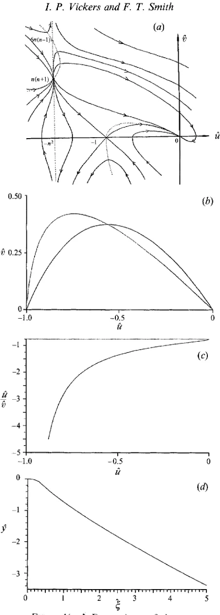
throughout here, as this is expected to be the most likely value and it represents the most common breakdown through (3.21). The ensuing numerical solution is shown in figure 4(b). The numerical method is extremely stable with respect to the grid structure, and the trajectory ends at the origin, thus supporting the phase-plane analysis. Furthermore, to support the earlier prediction for the ultimate form of zi as q+ co, the expression ti/$ was calculated as 6+0- and is plotted in figure 4(c) against its predicted limit value,--in.
The comparison seems affirmative. Generally, the numerical results support the analysis and hence, through the transformations (3.16), the existence of the desired solutions of (3.15). A direct computation of (3.15) has also been performed (Vickers 1993), yielding the results in figure 4 ( d ) .In summary, given (3.22), the local solution described above yields
I
U J ,ISJ cc 1pa-z)’n , IA,I 151(3n--2)/n at large
151
or, from (3.6a-c)IU- U J , IS-S,l oc IX-Xs)(2n-z)’n = IX-
x s p ,
(3.24a, b)IA -A,J K JX-XsJ@n-2)’n =
IX-
xsll+z’i
(3.24~) for small IX-XJ just outside the collapse region, with,f
defined in (3.22). Hence, inTo determine the far-field behaviour of j as
- _
FIGURE 4. (a) The phase plane for (3.17u, b). (b) The numerical solution of (3.23) from u^ = - 1 to u^ = 0. The dotted line represents (3.18), and the trajectory crosses this line with a zero gradient. (c)
162 I. P. Vickers and F. T. Smith
general, each of the streamwise velocity and the detached free shear-layer shape (and the local pressure due to (2.8dor e)) is predicted to stay finite but develop a singularity in its slope at X - X , = O + at the time T,-T= O + .
We turn next therefore to a numerical treatment of the full system (2.8a, b), (2.10a), (2.16).
4. Computational study using adaptive gridding
The analysis in the preceding section suggests that finite-time breakup of the mid- scale system (2.8a,b) and (2.104 b) or (2.16) exists. Turning then to a numerical treatment of (2.8a, b), (2.10a), (2.16) we describe in some detail a method of adaptive gridding which was developed to allow for this breakup solution in the numerical calculations.
The coordinate system ( X , T ) is transformed to a new coordinate system
(X,
T ) via the relation(4.1) for some smooth function g ( X , T ) which we may choose to meet our particular requirements. The function g(X, T ) is to be smooth, strictly monotonic increasing and, for the purposes of adaptive gridding, sensitive to the local solution activity. For the last requirement the function g should have small slope in regions of high solution activity, while to economize on computation the slope may be allowed to become relatively large in regions of slow solution variation. We take the option of g as a function of solution gradients (cf. the notion of equidistribution) and regard A@, T ) as the typical dependent variable. Clearly there are any number of possibilities for the description of the grid-transformation equation. Vickers (1993) studies three examples, and considers the consequences of each on the solution of the transformed numerical system of equations, with regions of high solution activity characterized by laA/aX/ -+ co and those of slow solution variation by laA/aAl + 0.
Of the three main examples for (4.1) studied in Vickers (1993), the most favourable has i?g/aX being set proportional to 1 - (i3A/aX)z, essentially, for simpler systems such as a Burgers equation A , + A A , K A,, for A(X, T ) . This choice of the grid-
transformation equation may appear somewhat ad hoc but the effect (Vickers 1993) on the efficiency and stability of the numerical computation is substantial. In addition the implementation of this technique, in the algebraic equations resulting from numerical simulation of the governing equations, is such that the grid-transformation equation may be altered by making only minimal adjustments to the program code, as in Vickers (1993). Comparisons between adaptive results and exact analytical solution for the Burgers equation are presented in the last reference, showing very close agreement even with the near presence of a shock and suggesting that an efficient approach is obtained. Given the encouraging results above, the numerical scheme that we used here incorporates the grid-transformation method just described. Hence the system of equations under consideration now is the transformed version of (2.8 a-c, e), namely
(4.2a)
(4.2b)
Breakup of unsteady subsonic or supersonic separating ,flows 163 where B = S + A is introduced to condense the notation, and we complete the system with the transformation equation
(4.2d)
The function r ( T ) is to be found, while the constants d, u, dz,s,d,,,, are fixed. The initial conditions considered here are
[U, S, A] = [0.1,0.1,0] +[1,0.8,0.4] exp { - 5(X+$)2} ( T = 0) (4.2e) to keep the eddy height S > 0 and ensure 4(U-A)-3S
>
0 initially, in view of (3.94 or (3.2a)-(3.3b).Together with the transformation (4.1), we substitute (4.2e) into (4.2d) which is then to be satisfied at T = 0, fixing ~ ( 0 ) .
In addition the form of (4.2a-c) suggests that we can impose two boundary conditions on A but only one on both U and S. On restricting the X-axis to the finite interval (- 1, l), it seems natural to choose
X
= - 1 as the boundary for prescribedvalues of U, S. This is in keeping with the idea that the incoming profile from
X
= - cois known. Thus from (4.2e) the boundary conditions are
Finally we close the initial-value problem with the fixed end-point conditions [ U , S , A ] ( - I , T ) = [ U , S , A ] ( - l , O ) , A(1, T ) = A(1,O). (4.2f)
( 4 . W which are implicit in (4.2f). g ( k 1, T ) =
k
1,164
I.
P.
Vickers and F. T. SmithI---
u
- .6
U
-1.0
Breakup of unsteady subsonic or supersonic separating flaws 165 The parameters CT,
p
in the discrete approximations for the first derivatives allow foran upwind-difference scheme, controlled by
for (4.3a,b) and
(4.4a)
(4.4h)
for ( 4 . 3 ~ ) .
In the system of algebraic equations the index i runs from 1 to N - 1 in ( 4 . 3 e d ) with the boundary conditions at 3 = - 1 (i.e. i = 0) given by (4.2.A g ) and substituted into
(4.3a-d) at i = 1. However, as U, S are predetermined at
x
= 1, and as we regard T ~ + ~ as a constant coefficient (see below), we require three more equations to close the system. Also, the artificial nature of the imposition of a finite downstream boundary implies that we are at liberty to choose a method by which to satisfy (4.2Jg) atx
= 1 (i.e. i = N ) . The most expedient method found involves the evaluation of (4.3b, d ) ati = N with backward differences enforced in ( 4 . 3 4 by setting CT = 1 at this point; and then the final equation is supplied by the elimination of the right-hand sides of
(4.3a, c) to obtain
where again backward differences in the z-derivatives are used, and the condition of fixed is applied. The last condition is used so that the difficult question of the discretization of the second derivatives at this end point is avoided.
Hence (4.3 a-d), with the above modifications at i = N , are solved for the unknown nodal values
Ui,i+l
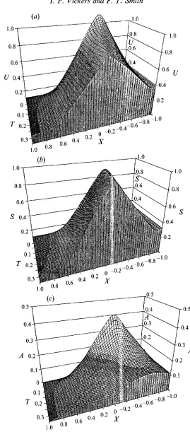
etc. at the ( j + 1)th time row using a global Newton linearization method, temporarily regarding qj+l as a constant coefficient. This method is enclosed within a secant loop to locate the value of qj+l which satisfies the second of conditionsInvestigations into grid-structure effects tended to suggest that the numerical method was more reliable, at least in the range of mesh sizes considered, when centred- difference approximations for the spatial derivatives in (4.3 a-c) were used. Results using this option are presented in figures 5-7. Other results are in Vickers (1993). From
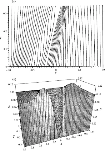
(4.2e), we see that the monitor function 4(U-A) - 3s (= E, say) takes the value 0.1 identically at T = 0. According to $3, E then tends to zero at a finite-time breakup subsequently. A plot of the evolution of E is given in figure 6(h), from which it seems very evident that the monitor function E tends to zero at a finite value of
T,
X
(orX),
in line with the analysis in §3. A plot of the locus of the minimum value of E at each time step, in figure 6(c), suggests that E first becomes zero at(X,
T ) = (Xs, TJ M (0,0.34). The numerical integration was usually terminated near this point in order to present the results in figures 5 and 6. However, if allowed to(4 2
d.
FIGURE 5. (a) A plot of the scaled streamwise velocity profile U from the numerical solution of the mid-scale separating-flow system (4.2~-e). Here
Ax=
0.04, AT = 0.001, d, = 0.2, d2,.7 = 0.1,166
(4
-0.3 -
-
0.2 -
T
0.1
-
-
0
-1.0
I.
P.
Vickers and F. T . Smith-1
I .0.5 1.0
1
.o
FIGURE 6(a,b). For caption see facing page.
Breakup of unsteady subsonic or supersonic separating J ~ O W S 167
0.1 0.2 T
0.3
FIcium 6. (a) The evolution of grid nodes in figure 5. (b) A plot of E (= 4 ( U - A ) - 3 S ) calculated from the results displayed in figure 5. (c) The locus of the minimum value of E at each time step. ( d ) Plotting the slope of the solution in figure 5(a), calculated from the centred-difference ratio AU/Ag at each internal grid point.
168 I.
P.
Vickers and F. T. SmithBreakup of unsteady subsonic or supersonic separating flows 169
(4
J
0.7 -
0.6 -
0.5 1
0.4 1
0.3 1
0.2 -
0.1 -
T I
0 -.
-0.1 -0.5 0
X
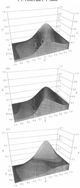
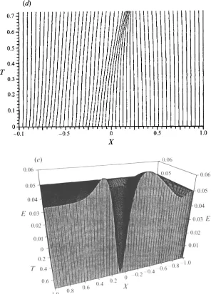
FIGURE 7. Results obtained using initial conditions in which U , S, A in (4.2e) are all halved. (a) A plot of the scaled streamwise velocity profile U from the numerical solution of the mid-scale separating- flow system. Here AX= 0.04, AT = 0.001, dl = 0.2, d2,s = 0.1, d2,b = d2,A = 0. (b) As (a) but for the scaled shear-layer shape S . (c) As (a) but for the scaled boundary-layer displacement -A. ( d ) The evolution of grid nodes in (ac). (e) A plot of E (= 4 ( 1 / - A ) - 3 S ) calculated from the results displayed in (a-c).
170
I.
P . Vickers and F. T. Smith5. Further comments
To recap first, this study has been concentrated on the solution of the partial- differential equations (§
2)
governing mid-scale unsteady separating flow, which occurs closer to the separation point than does the full-scale flow of Brown et al. (1988). See the range (1. l), (1.2). The governing equations involved are effectively inviscid, with viscous effects assumed to be confined mainly to the thin detached shear layer and to a thin wall layer. The predominantly inviscid nature might be expected to be correct physically as some evidence suggests that full transition usually takes place on a convective rather than a diffusive timescale. In particular that agrees with the findings of Smith (1988), Stewart & Smith (1992), Smith & Bowles (1992). The numerical solutions in $4 and others presented in Vickers (1993) then agree broadly with the analysis in $3 proposing a finite-time breakup of the mid-scale flow solution, with the normalized streamwise velocity U and eddy width S developing infinite slopes in a manner analogous with that in Smith (1988). The breakup contrasts with the response in the full-scale separating flow of Brown et al. (1988) which results usually in a local eruption into the main stream.The investigation in @3 and 4 addresses supersonic external flow, where the pressure-displacement law is easier to handle than is the subsonic case, but we would expect the conclusions in $53 and 4 on finite-time breakup to apply also to subsonic flow, since the orders of magnitude, and the expansions, involved are the same locally and indeed the influence of the pressure-displacement law diminishes at breakup, as a comparison of $3.1, $3.2 indicates. Further study might also consider the response in the viscous sublayers, at or prior to the breakup, non-uniform distributions of vorticity (cf. §2), increased thickness of the detached shear layer (cf. the range (1. l), (1.2)), and three-dimensional effects, to examine the generality of the mid-scale breakup found here. Other parameter ranges, for example with upper-branch scalings, are also of interest
.
Physically, perhaps the most notable point of the solutions in 993 and 4 is that the increment in the boundary-layer displacement K A - A , becomes small at breakup, as shown in (3.6~) and in the figures. Thus the overall boundary layer acts locally as if there were almost no net displacement effect, but with the eddy width retaining its original order of magnitude, since S remains of order unity. The eddy’s streamwise velocities K U, can then be positive or negative according to (3.9a, h), which affects the
viscous wall layer of course. If U, is locally positive, with So small, say, so that C, z U,, that would tend to indicate a reattachment taking place, possibly linking with the experimental observations described in
5
1. The above reduction in the displacement effect provides a related link with the experiments. Also on the physical or applications side, the conditions (3.9a, b) themselves act as a form of breakup criterion for separating Bow, cf. the monitor function E in $4. In fact, they can be shown to be equivalent to the interactive breakup criterion of Smith (I 988), namely that ifI
[V( Y ) - C,]-’dY = 0Breakup of unsteady subsonic or supersonic separating fzows 171 parameter range (l.]), (1.2), as well as for the original system (2.2a-e). The ensuing behaviour more locally following the scale changes then depends on where the parameters lie, within the range (1. l), (1.2), cf. the discussions in Smith (1993), Hoyle
et al. (1991) concerning the advent of normal pressure gradients and local vortex formations.
Theoretically, in addition to the points in the previous paragraph, the study appears to confirm that the finite-time breakup singularity in Smith (1988) occurs quite widely, albeit in a modified form in the present separated-flow context. Other recent examples are in Peridier et al. (1991~1, b), Smith & Bowles (1992), Hoyle & Smith (1994), and work in preparation by
R.
1. Bowles and F. T. Smith, showing agreement with computations and with experiments and extensions to three-dimensional motions. Similar extensions to vortex-sheet motions may also apply.Computationally, the adaptive-grid method introduced in $4 seems to be a simple yet quite effective method of implicit solution-dependent deployment of the grid. The treatment, described in $4 but in more detail in Vickers (1993), tends to support such a view and it is felt that the effective deployment of grid nodes maintains acceptable accuracy of the numerical solution even near the breakup. Discretization errors consist of expressions involving local derivatives of the solution which remain slowly varying even in regions of high solution activity because of the grid transformation (4*1). The neat capturing of the singular breakup solution shown in
$4
(e.g. figures 5-7) is encouraging, and the application of this method to other numerical problems, such as for full interacting boundary layers, seems possible and promising.Thanks are due to SERC for support of I.P.V., and for computational facilities, to ARO (grant no. DAAL-03-92-60040 through Dr T. Doligalski) for support of F. T. S., and to Professors R. J. Bodonyi, A. T. Conlisk, E. R. Johnson, A. P. Rothmayer, J. D. A. Walker, G. Wilks and Dr M. Barnett for valuable discussions on various aspects of the research. The referees’ comments are acknowledged gratefully.
REFERENCES
BROTHERTON-RATCLIFFE, R. V. & SMITH, F. T. 1987 Complete breakdown of an unsteady interactive
BROWN, S. N., CHENG, H. K. & SMITH, F. T. 1988 Nonlinear instability and break-up of separated
BURSNALL, W. J. & LOPTIN, L. K. 1951 N A S A T N 2338. CATHERALL, D. 1991 Roy. Aero. Estab. Tech. Rept. 91021.
CONLISK, A. T., BURGGRAF, 0. R. & SMITH, F. T. 1987 Nonlinear neutral modes in the Blasius
DOVGAL, A. V., K ~ Z L O V , V. V. & SIMONOV, 0. A. 1987 In Boundary-Layer Separation (ed. F. T.
DRAZIN, P. G. & REID, W. H. 1981 Hydrodynamic Stability. Cambridge University Press. DUCK, P. W. 1985 Laminar f l o ~ over unsteady humps: the formation of waves. J . FluidMech. 160,
465.
EISEMAN, 1’. R. 1987 Adaptive grid generation. Comput. Methods Appl. Mech. Engng 64, 321.
FIDDES, S. P. 1980 A theory of the separated flow past a slender elliptic cone at incidence. AGARD Paper 30.
GASTER, M. 1966 AGARD ConJ Proc. 4, 819 (Also Aeronaut. Res. Counc. Rep. & Mem. 3595, 1969).
GAULT. D. E. 1955 N-4SA T N 3505.
boundary layer (over a surface distortion or in a liquid layer). Mathematika 34, 86.
flow. J . Fluid Mech. 193, 191.
boundary layer. Forum on Unsteady Separation. ASME, FED vol. 52, p. 119.
172 I.
P.
Vickers and F. T. SmithHALL, P. 1982 On the nonlinear evolution of Gortler vortices in growing boundary layers. J. Znst.
HAWKEN, D. F., HANSEN, J. S. & GOTTLIEB, J. J. 1991 A new finite-difference solution-adaptive
HOYLE, J. M. & SMITH, F. T. 1994 On finite time break up in 3D unsteady interacting boundary
HOYLE, J. M., SMITH, F. T. & WALKER, J. D. A. 1991 On sublayer eruption and vortex formation.
KACHANOV, Y. S., RYZHOV, 0. S. & SMITH, F. T. 1993 Formation of solitons in transitional
KOROLEV, G. L. 1980 Numerical solution of asymptotic problem on separating laminar boundary
KOZLOV, V. V. 1987 In Boundary-Layer separation (ed. F. T. Smith & S. N. Brown). Springer. MEHTA, U. B. 1977 Unsteady aerodynamics. In AGARD Con$ Proc. 227, Paper 23.
MESSITER, A. F. 1983 Truns. ASME. E: J. Appl. Mech. 50, 1104.
MEZARIS, T. B., TELIONIS, D. P., BARBI, C. & JONES, G. S. 1987 Separation and wake of pulsating laminar flow. Phil. Trans. R. Soc. Lond. A 322, 493.
MOORE, D. W. 1979 The spontaneous appearance of a singularity in the shape of an evolving vortex sheet. Proc. R. Soc. Lond. A 365, 105.
MUELLER, T. J. 1984 AIAA Aerospace Paper 84-1617.
MUELLER, T. J. & BATILL, S. M. 1980 AIAA Aerospace Paper 80-1440.
PERIDIER, V. J., SMITH, F. T. &WALKER, J. D. A. 1991 a Vortex-induced boundary-layer separation. Part 1. The unsteady limit problem Re + co. J . Fluid Mech. 232, 99.
PERIDIER, V. J., SMITH, F. T. & WALKER, J. D. A. 1991 b Vortex-induced boundary-layer separation. Part 2. Unsteady interacting boundary-layer theory. J. Fluid Mech. 232. 133.
SAFFMAN, P. G. & SCHATZMAN. J. C. 1982a Stability of a vortex street of finite vortices. J. Fluid Mech. 117, 171.
SAFFMAN, P. G. & SCHATZMAN, J. C. 19826 An inviscid model for the vortex-street wake. J . Fluid
Mech. 122, 467.
SMITH, F. T. 1977 The laminar separation of an incompressible fluid streaming past a smooth surface. Proc. R. Soc. Lond. A 356, 443.
SMITH, F. T. 1979 On the non-parallel flow stability of the Blasius boundary layer. Proc. R. SOC.
Lond. A 366, 91.
SMITH, F. T. 1982 On the high Reynolds number theory of laminar flows. IMA J. Appl. Maths 28,
207.
Maths. Applies. 29, 173.
method. Phil. Trans. R. Soc. Lond. A 341, 373.
layers. Proc. R. Soc. Lond. A (to appear).
Compub. Ph,vs. Commun. 65, 151.
boundary layers: theory and experiment. J. Fluid Mech. 251, 273.
layer at a smooth surface. Sci. J. TSAGZ 11 (2), 27.
SMITH, F. T. 1984 Theoretical aspects of the steady and unsteady laminar separation. AZAA Paper
841582.
SMITH, F. T. 1986a Two-dimensional disturbance travel, growth and spreading in boundary layers.
SMITH, F. T. 19866 Steady and unsteady boundary-layer separation. Ann. Rev. Fluid Mech. 18, 197. SMITH, F. T. 1987 Nonlinear effects and non-parallel flows; the collapse of separating motion. In
Stability of Time-Dependent and Spatially Vurying Flows (ed. D. L. Dwoyer & M. Y. Hussaini). Springer. (Also Utd Tech. Res. Cent., E. Hurtffford, CT, Tech. Rep. UT85-55.)
SMITH, F. T. 1988 Finite-time break-up can occur in any unsteady interacting boundary layer.
Mathematika 35, 256.
SMITH, F. T. 1993 Theoretical aspects of transition and turbulence, AZAA J. 31, 2220-2226. SMITH, F. T. & BODONYI, R. J. 1985 On short-scale inviscid instabilities in flow past surface-mounted
obstacles and other nonparallel motions. Aeronaut. J. R. Aeron. Soc., June-July.
SMITH, F. T. & BOWLES, R. I. 1992 Transition theory and experimental comparisons on (I) amplification into streets and (11) a strongly nonlinear break-up criterion. Proc. R. SOC. Lond.
A 439, 163.
SMITH, F. T. & BURGGRAF, 0. R. 1985 On the development of large-sized short-scaled disturbances in boundary layers. Proc. R. Soc. Lond. A 399, 25.
SMITH, F. T., DOORLY, D. J. & ROTHMAYER, A. P. 1990 On displacement-thickness, wall-layer and