Using Vicon system and optical method to evaluate inertial
and magnetic system accuracy
P. Grenet1,2,a,PhD student , F. Mansour1,DRT student 1
Cea LETI-Minatec, 17 rue des Martyrs, 38054 Grenoble cedex 9, France 2
Movea SA BHT, 7 Parvis Louis Néel, 38040 Grenoble, France
Abstract. MEMS are being more accessible thank price and energy consumption. That explains the democratisation of attitude control system. Sensors found in attitude control system are accelerometers, magnetometers and gyrometers. The commercialised solutions are expensive and not optimised in sensors number and energy consumption. Movea’s system is based on low cost sensors, number optimisation and low energy consumption. It is constituted of wireless attitude control system named MotionPOD. The system has two modes: the simulation mode and the reconstruction mode, even for cinematic motions. Movea’s system is seen as a black box which becomes as entries measurements for reconstruction mode and body segment orientation for simulation one. In body motion reconstruction Vicon system is usually used because of its accuracy. With markers position it is easy to compute the orientation of each body segment if we have put enough markers. That is why Vicon system may be a good etalon for the Movea’s system. We present practical approach of the characterisation of Movea’s system and its validation. Thereby we will present criterion useful to evaluate the reconstruction accuracy. Moreover we will insist on optical methods used to extract the interesting data from Vicon.
Movea’s System is based on attitude control system in order to compute body segment orientation for static but also cinematic motion in Earth’s frame. Its orientation estimation is evaluated through magnetometers and accelerometers. To have a better estimation we could also use the gyrometer version but our goal is to extract the maximum information from the AM version (Accelerometer Magnetometer), for it exhibits a lower cost.
An accelerometer is a sensor which gives an evaluation of acceleration due to no gravitational forces in its own frame. So with no acceleration this sensor gives a measurement of gravitation. Indeed the mechanical equation gives us the result:
* M a=∑F
(1)
_ 0
total no gravitationnal gravitationnal
a =a +a =
(2)
_ * 0
no gravitationnal
F F M G
∑ =∑ + =
(3)
a
e-mail : [email protected]
With
: Mass of the accelerometer : Force exerced on the accelerometer : Acceleration of accelerometer
: Gravitationnal field
M F a G So _ * no gravitationnal
a = - M G
(4)
And with acceleration, we have
_ *
no gravitationnal total
a =a - M G
(5)
So in equations (4) and (5), we see, whereas the accelerometer is not sensitive to gravitational forces, its measure depends on gravitation by “negative image”.
The first accelerometers MEMS were only scalar sensors which measure only along one axis and we had to put three mono-axes sensors to have 3D measurement. Yet the manufacturers send native three axis accelerometers.
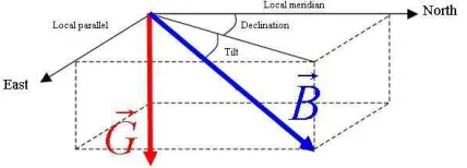
A magnetometer estimates the magnetic field in its own frame. The magnetic field on Earth is a stationary field in regard of duration of the experiments we do. In our latitude (France), it’s a vector oriented at 30° from the vertical in direction of the magnetic north.
Fig. 1 : Schema of gravitational and magnetic earth's field
Gand
Bare respectively the gravitational earth’s field and the magnetic earth’s field
Like for the accelerometers first MEMS were mono-axis and yet we can work with native three axes microchips.
A gyrometer measures angular velocity in its own frame. MEMS gyrometers have appear more recently, so native three axes are just available. Moreover they are a little bit more expensive and bigger energy consumer, but with time differences are being always smaller. In our study we try to reconstruct orientation with as less as possible sensor modality and so we don’t use gyrometers.
So the system we study is composed of many attitude control systems witch are put on all body segment we want to determine orientation. But we can’t only study extremities segment: for instance if we are interested on evaluated forearm orientation we have to put also attitude control systems on arm and shoulder.
14th International Conference on Experimental Mechanics
(and gyrometer). So gyrometers are optional for the both functionalities, but in this study we don’t use this modality because the purpose is to evaluate the capacity of AM cinematic reconstruction. “Cinematic” must be understood as “with no-negligible acceleration”: so we are in the case of the equation (5).
Fig. 2 : Schema of Movea's system mode There are two modes: simulation and reconstruction. The two modes need parameters: position and orientation of sensor in segment frame
For this presentation Movea’s system is seen as a black box and we only present it from user point of view.
1. Experimental process
In order to evaluate the system accuracy we did some experiments in ex-LMS Poitiers (P’ Institute) with a Vicon system composed of ten infrared cameras and a force platform.
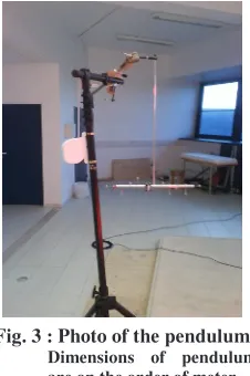
The first experiment we made is a very simple system: a pendulum which has one degree of freedom (rotation) and the second was a pendulum with three degrees of freedom (three rotations).
Fig. 3 : Photo of the pendulum Dimensions of pendulum are on the order of meter
Fig. 4 : Pendulum with the MotionPOD On the photo, we see the different markers and the MotionPOD fixed on the pendulum
On this bar we fixed a MotionPOD, a wireless sensor from Movea, which is composed of a three axes accelerometer and a three axes magnetometer.
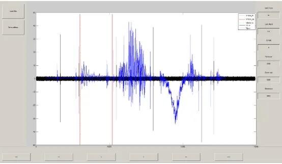
Fig. 5 : Graph representing force platform signal with the first component of accelerometer
The two signals on the graph are not good synchronize to show corresponding peaks on the both signals. We can see the red line which cut the interesting part of signal and the dot point line which indicate the reference of rotation (where rotation is set to identity). Buttons below are used to modify the synchronisation offset.
One base of the support is placed on the force platform, so when the support is shaken we can detect it on the platform signal and the accelerometer. This method gives the possibility to synchronize signals from Vicon system and Movea’s System (Fig. 5).
2. Optical Method
The purpose of optical methods used here is to compute the orientation of a segment during the experiment in order to be able to compare simulation from Movea’s black box with real measures and orientation itself with orientation estimated by Movea’s black box.
The first problem is to interpolate Vicon's data to find the position of the optical markers when they are osculated. In order to do it we used the hypothesis that any length between points of a solid is constant during the time. So we compute a relative distance matrix between each pair of markers from a same solid thanks to a calibration sequence by using the following calculus:
Mat_relative_dist(i, j)= distance(Marker(i),Marker(j)) for j i Mat_relative_dist(i, j - 1) = distance(Marker(i),Marker(j)) for j > i
<
(6)
To find the position of an osculated point, we optimize (7) the estimation of its position using the criterion given by the equation (8).
marker(i)min f(marker, Mat_relative_dist)
(7)
i-1
k=1 markers number
k=i+1
f(marker, Mat_relative_dist)= (distance(marker(i),marker(k))- Mat_relative_dist(i,k))²
+ (distance(marker(i),marker(k))- Mat_relative_dist(i,k))²
∑
∑
(8)
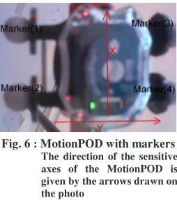
The second problem is to determine sensor (MotionPOD) frame and more precisely the change frame matrix between Vicon frame and MotionPOD frame. Therefore we put markers on MotionPOD following its axes.
Fig. 6 : MotionPOD with markers
The direction of the sensitive axes of the MotionPOD is given by the arrows drawn on the photo
So we have an image of the direction of MotionPOD principal axes. For further accuracy we record this image during many samples. This sequence is called the geometric calibration sequence. With this axes we can compute the change frame matrix by using Gramm-Schmidt orthonormalization:
mean(Marker(1) - Marker(2))+ mean(Marker(3) - Marker(4)) X =
mean(Marker(1) - Marker(2))+ mean(Marker(3) - Marker(4)) mean(Marker(1) - Marker(3))+ mean(Marker(2) - Marker(3)) Y =
mean(Marker(1) - Marker(3))+ mean(Marke
( , )
_ _ [ , , ]
r(2) - Marker(3)) Y - dot(X,Y)* X
Y =
Y - dot(X,Y)* X
Z cross X Y
Mat change frame X Y Z
= =
(9)
Marker(i)is representing the position of the marker numberiin Vicon's frame.
The third problem is to compute the rotation matrix of the pendulum during time. To do this we use a classical solution:
For each sample we compute all the vectors available on the solid using a pair of markers. Then we use the algorithm QUEST to find the orientation. The QUaternion ESTimation algorithm is an orientation estimation algorithm developed by the NASA which determines orientation using stars directions ([1]). It is based on quaternion eigenvalue equation formulation. Each vector observation is weighted to give more importance for best vector measurements. QUEST algorithm is also usually used for static AM reconstruction (with no acceleration).
The last problem is to determine the position of the sensors on the pendulum and particularly the distance from rotation center. To obtain this parameter we use an ingenious formulation of the last square equation:
²
, i²
i Marker(i)- Rot_Point ² R
" =
(11)
This parameter is given to Movea’s system by a position of the sensor in the segment (pendulum here) frame.
3. Comparison Criterion
To compare simulation and real measures we chose a natural criterion: the difference between the two signals.
To compare the estimation of orientation given by Movea’s system with the one given by Vicon we use two criterions: the first one is an angular difference (13), and the second one is a position difference (14).
1
_ _ _ _ * _ _
Mat Rot residual=Mat Rot Vicon Mat Rot Movea-
(12)
[Angular diff Vect diff_ , _ ]=Matrice2angleVect Rotation residual( _ )
(13)
These two equations (12) and (13) show us how the angular criterion is computed: we represent the residual rotation by the formalism angle-vector and this angle is our criterion.
( _ )
Distance = ViconMarkerPosition - ReconstrutMarkerPosition Rotation Movea
(14)
The distance computed on the equation (14) is the second criterion chosen.
4. Results
The results are good for the simulation mode. We have a difference lower than 10 %. On the two figures below, Fig. 7, we can see a very good concordance between simulation and real measurement.
Fig. 7 : Accelerometer (left) and Magnetometer (right): Simulation and Measure
On graphs the real measure is in thin line and simulation in thick line
The signal being very long we just have here a zoom for some samples, the little graphs showing us what we see in regard of the complete signal
The slight difference for the acceleration is due to vibrations of the pendulum (translations) which are not considered by Movea’s system. For the magnetic measurement and simulation we see a little difference on top (or down) of sinusoids that can be due to magnetic perturbations or inaccuracy in sensor orientation estimation.
Fig. 8 : Comparison between static algorithm and Movea's algorithm On the graph, we see Movea’s algorithm is more efficient than static algorithm. In term of mean Movea’s algorithm have angular error of 1,8° (with a standard deviation of 1,4°) whereas static algorithm have one of 17,1° (with std of 16,9°).
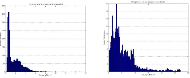
On figures below, Fig. 9, we see the histogram of angular error. The two figures show results for different tests, the first is very good; it corresponds to a quite simple motion, whereas the second corresponds to a very complex motion. The error is also enlarged by dynamic error and bad synchronization. Indeed the faster the motion is, the greater the influence of bad synchronization and dynamic error is.
Fig. 9 : Histogram of angular error: simple (left) and complex (right) motion The simple motion excites only one DOF and is not very fast
The complex motion excites three DOF and had very fast sequence
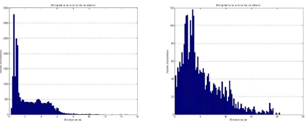
Fig. 10 : Histogram of distance error: simple (left) and complex (right) motion The motions given here are the same as the ones on Fig. 9
It has the same look as the angular error histogram, what is not surprising because the position of markers depends directly on angular estimation. We can compare the biggest error with the dimension of the pendulum: it correspond to 20% of the pendulum dimension (20 cm in regard to 1m), this is a big error (in terms of distance) but a very short one (in terms of time) (1 or 2 samples).