EXISTENCE THEOREMS FOR TRAPPED MODES

Journal of Fluid Mechanics

http://journals.cambridge.org/FLM

Additional services for Journal of Fluid Mechanics:

Email alerts: Click here Subscriptions: Click here Commercial reprints: Click here Terms of use : Click here

Existence theorems for trapped modes

D. V. Evans, M. Levitin and D. Vassiliev

Journal of Fluid Mechanics / Volume 261 / February 1994, pp 21 ­ 31 DOI: 10.1017/S0022112094000236, Published online: 26 April 2006

Link to this article: http://journals.cambridge.org/abstract_S0022112094000236 How to cite this article:

D. V. Evans, M. Levitin and D. Vassiliev (1994). Existence theorems for trapped modes. Journal  of Fluid Mechanics, 261, pp 21­31 doi:10.1017/S0022112094000236

Request Permissions : Click here

J. Fluid Mech. (1994), vol. 261, pp. 21-31 Copyright 0 1994 Cambridge University Press

21

Existence theorems for trapped modes

By D. V. EVANS’, M. LEVITIN2 A N D D. VASSILIEV3

School of Mathematics, University of Bristol, University Walk, Bristol BS8 lTW, UK

*

Department of Mathematics, Heriot-Watt University, Riccarton, Edinburgh EH14 4AS, UK School of Mathematical and Physical Sciences, University of Sussex, Falmer,

Brighton BN1 9QH, UK

(Received 17 February 1993)

A two-dimensional acoustic waveguide of infinite extent described by two parallel lines contains an obstruction of fairly general shape which is symmetric about the centreline of the waveguide. It is proved that there exists at least one mode of oscillation, antisymmetric about the centreline, that corresponds to a local oscillation at a particular frequency, in the absence of excitation, which decays with distance down the waveguide away from the obstruction. Mathematically, this trapped mode is related to an eigenvalue of the Laplace operator in the waveguide. The proof makes use of an extension of the idea of the Rayleigh quotient to characterize the lowest eigenvalue of a differential operator on an infinite domain.

1. Introduction

The existence of trapped modes above a long submerged horizontal circular cylinder of sufficiently small radius, in deep water, was proved by Ursell(l951) over forty years ago. At about the same time Jones (1953), using deep results on unbounded operators, extended Ursell’s proof to a wide class of submerged horizontal cylindrical obstacles in finite water depth and also removed the requirement that the obstacle be small. Jones’ results, as applied to the water-wave problem, formed just a small part of his paper in which a number of general results were obtained concerning the spectrum of the Laplace operator satisfying certain boundary conditions given on semi-infinite domains. Possibly because of the difficult nature of the paper, little attention appears to have been paid to these results in the acoustic or water-wave literature.

Recently, there has been a revival of interest in predicting those situations in which trapped modes, or acoustic resonances, as they are described in the acoustic literature, might occur, because of their importance in, for example, the design of turbomachinery. A good review is provided by Parker & Stoneman (1989) who describe a wide variety of engineering applications where acoustic resonances have been observed and measured.

22

separation of the depth factor in the water-wave problem reduces it to the acoustic waveguide problem. Again Callan, Linton & Evans (1991) using methods similar to Ursell (1951) proved that an antisymmetric trapped mode existed for a sufficiently small circular cylinder midway between parallel walls of finite extent whilst Ursell(l99 1) generalized this result to the axisymmetric case of a small sphere on the centreline of a circular tube of infinite extent. Evans (1992) proved the existence of trapped modes in the case of a sufficiently long vertical plate positioned parallel to and midway between the walls of the channel. The corresponding acoustic problem to this was observed by Parker (1966) who also used numerical techniques to estimate the acoustic resonant frequencies. Evans, Linton & Ursell (1993) considered the case of a sufficiently long vertical plate off the centreplane of the channel, where it is not possible to separate the problem into solutions symmetric or antisymmetric with respect to the centreplane, and showed that in this case also a trapped mode existed which, since the problem allowed all positive frequencies, had a corresponding trapped mode frequency embedded in the continuous spectrum. Finally, Linton & Evans (1992) used an appropriate Green’s function to construct a homogeneous integral equation for the trapped modes in the case of a cylinder of fairly general cross-section and showed that the trapped mode frequencies agreed numerically with the previous results for the circular and rectangular cross-sections.

In each of the water-wave problems described above the alternative interpretation of a trapped mode in an acoustic waveguide can be made and for definiteness we shall adhere to this interpretation in what follows.

In the next two Sections we shall prove, using a variational formulation, that a trapped mode exists in a two-dimensional acoustic waveguide of fairly arbitrary cross- section. We shall identify a trapped mode frequency as an eigenvalue of the Laplace operator on an unbounded domain and we shall establish the existence of the smallest such eigenvalue by making use of a theorem in which the eigenvalue is described in terms of the Rayleigh quotient. This theorem, which is not proved here, provides an extension to certain differential operators on unbounded domains having combined discrete and continuous spectra, of the simple Rayleigh quotient characterization for the lowest eigenvalue of differential operators on bounded domains where the spectrum is purely discrete.

It will become clear from the method of proof that the method can be adapted to other situations where trapped modes are anticipated, including the case considered by Ursell(l991). To illustrate this we indicate in 54 how the method can be applied to the case of a two-dimensional acoustic waveguide containing symmetric indentations on opposite sides.

2. Mathematical statement of the problem and some basic mathematical facts

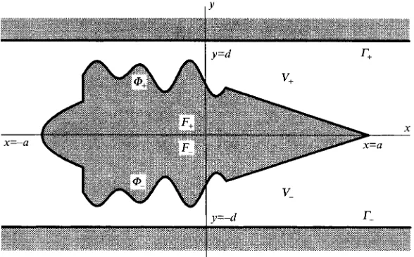
We consider a two-dimensional acoustic waveguide G = {(x,y):lyl

<

d } the boundary of which is represented in Cartesian coordinates {x, y } by two parallel lines

Ti

= { y = +d}. The waveguide encloses an obstruction I; which is symmetric about

the centreline y = 0 of the waveguide, but otherwise has arbitrary shape; the boundary @ = @+

u

@- of the obstruction is assumed to be piecewise smooth and parametrized in the form ds, = {(x,y):x = X(s), y = f Y(s), 0

<

s d L}, where X(s), Y(s) are continuous, piecewise infinitely smooth functions such that Xi2

+

Yi2

=

1,0

<

Y(s) < d, Y(0) = Y(L) = 0, X(0) = -a, X ( L ) = a (see figure 1). The only conditions on the

Existence theorems for trapped modes 23

l Y

FIGURE 1. Waveguide with obstruction (Y(s)

+

0).

not go through the same point twice). For technical reasons we also assume that Y’(s

+

0) - Y’(s - 0) < 2 for all s E (0, L) (there are no cusps protruding inside the

obstacle). We denote by 2agf X(L)-X(0)

>

0 the length of obstruction. By S(x) we denote the inverse function to the function X(s) (i.e. S(x) is the root of the equation x =

X(S(x))

if this root is unique; on the parts of the boundary where X’(s)

=

0 we put

for definiteness S(x)

zf

min {s: x = X(s)}). Note that the case Y(s)

=

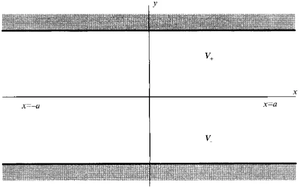
0 (infinitely thin obstruction along the centreline, see figure 2) is included in our general scheme.

We consider the following boundary value problem for a potential $(x,y): ( d + h ) $ = 0 for ( x , y ) ~ V = G\F, (2.1)

(2.2)

- =

a4

0 for ( x , y ) ~ I ‘ + , aY

$ + O for IxI+co, lyl d d . (2.4) In (2.3) a/an denotes the derivative with respect to the normal vector to the boundary of the obstruction; (2.3) is assumed to be fulfilled on the smooth parts of the boundary of the obstruction, because at the vertices the normal is undefined. In (2.1) I/ is the volume occupied by the acoustic medium, and h is a spectral parameter which is related to the frequency of acoustic vibration o by h = 02/c2, c being the velocity of sound. Convergence in (2.4) is understood as uniform convergence over IyI

<

d. Equations (2.1)-(2.4) arise after separating out the time factor exp (iot) in the full time-dependent problem, the actual potential being Re($exp(iot)). At the same time, as in Evans &

Linton (1991) and Callan et al. (1991) these equations describe the water-wave problem in which the water is of depth H and the obstruction extends throughout the entire depth. In this case the depth factor coshha(z+H) is also separated out ( z being the vertical coordinate) and h is the unique positive root of

I Y

x=-u x=a

V-

I

FIGURE 2. Waveguide with obstruction (Y(s) =- 0).

We seek values of h for which non-trivial solutions $(x, y ) of (2.1)-(2.4) exist. These values correspond to the so-called trapped modes with frequency w.

We shall be mostly interested in solutions which are antisymmetric about the axis y = 0, i.e. $(x, y ) = --$(x, -y). It is easily seen that such solutions (which we shall

denote by $"(x, y)) satisfy the following auxiliary problem :

( A +A) $" = 0 for (x, y ) E V, = G+\F+, (2.5)

$a = 0 for ( X , Y ) E @ ~ ,

$a+O for IxI--tco, O < y < d .

Here G, = {(x,y):O

<

y

<

d}, = { ( x , y ) : y = 0, X E ( - G O , -a]

u

[a, +GO)},

F+

is the upper half of the obstacle F, and V+ is the volume occupied by the acoustic medium. Convergence in (2.9) is understood as uniform convergence over 0

<

y

<

d. The essential new element in comparison with the initial problem (2.1)-(2.4) is condition (2.8), which allows us to continue the solution $" antisymmetrically about the line y = 0. Later on we will show that condition (2.8) also plays a crucial role for the existence of trapped modes.

In order to conclude the rigorous mathematical statement of the problems (2.1)-(2.4) and (2.5)-(2.9) we should describe appropriate classes of functions in which we seek the potentials q5 and q5", respectively. Both from the mathematical and physical points of view it is reasonable to require the potentials to be infinitely diferentiable at all internal points of the region V (respectively, V,) occupied by the acoustic medium as well as up to the smooth parts of the boundary. Since the boundary @+ of the obstruction is assumed to be only piecewise smooth, we shall require the potentials $ and $" to be

continuous at all the vertices of the lines @ and @+, respectively.

Existence theorems for trapped modes 25 requirements on the solution as problem (P) and to the problem (2.5)-(2.9) as problem

(Pa>.

Now we introduce the important concepts of continuous and point spectra of our problems.

We shall say that a number h is an eigenvalue of the problem (P) or (Pa) (in other words, h belongs to the point spectrum of the problem (P) or (Pa)) if for this h there exists a non-trivial potential q5 or which satisfies (2.1)-(2.4) or (2.5)-(2.9), respectively.

We shall say that a number h belongs to the continuous spectrum of the problem (P)

or (Pa) if for this A there exists a non-trivial potential q5 or #a which satisfies (2.1)-(2.3)

or (2.5)-(2.Q grows at x-infinity not faster than polynomially, but does not vanish at x = f co. In other words, here we allow the potential q5 (or @) to behave at x-infinity, for example, as Ix(", n 2 0, but do not allow it to behave at x-infinity as exp 1x1. Note that the potentials appearing in our definition of the continuous spectrum are not really solutions of our problems (P) or (Pa) because they do not satisfy the decay conditions (2.4) or (2.9). However, consideration of such non-decaying solutions is essential for the understanding of our problems in terms of spectral theory of operators.

From the physical point of view, modes (potentials) corresponding to eigenvalues do not radiate towards x = & co or receive radiation from x = f co, whereas radiation to

x = & co occurs in modes corresponding to points of the continuous spectrum. We shall call the potentials involved in the definition of eigenvalues eigenfunctions or

trapped modes; the latter name is more physical because it reflects the fact that these

potentials are localized near the obstacle, while away from the obstacle they rapidly decay. The potentials involved in the definition of the continuous spectrum can be called eigenfunctions of the continuous spectrum or propagating modes.

Our main aim is to show that trapped modes always exist, i.e. that problem (P)

always has at least one eigenvalue. As we shall see the main difficulty in proving this fact is that this eigenvalue is necessarily embedded in the continuous spectrum of the problem (P), which prevents us from using the standard functional analysis technique. Normally, eigenvalues embedded in a continuous spectrum are a very rare occurrence; their study requires special methods and there must be special reasons for there existence. In our particular case this special reason is the symmetry of the problem (P)

with respect to the axis y = 0. This symmetry will allow us to reduce our consideration to the more simple problem (Pa) for which the continuous spectrum starts higher and, as a result, the eigenvalue in question lies below the continuous spectrum.

The following result is well-known (see, e.g. Jones 1953; Evans & Linton 1991; and for a more general discussion Birman & Solomjak 1987 and Sanchez-Hubert &

Sanchez-Palencia 1989).

LEMMA 2.1. The continuous spectrum of the problem (5') is the semi-interval [0,

+

co).

The continuous spectrum of the problem (Pa) is the semi-interval [n2/(4d2),

+

a).

Physically, Lemma 2.1 means that in the full problem (P) for any positive h there exists a mode of vibration radiating to x = co and receiving radiation from x = & 00,

whereas in the antisymmetric problem (Pa) no radiation is possible when h < n2/(4d2). The frequency 52 = CA; corresponding to A = n2/(4d2) (the lower point of the

continuous spectrum of the problem

(Pa)),

is called the cut-of frequency.

The rigorous mathematical proof of Lemma 2.1 lies beyond the scope of this paper (see references above). Note, however, that it can be obtained directly from our definitions using separation of variables for sufficiently large 1x1.

D. V. Evans, M . Levitin and D. Vassiliev

then it is also an eigenvalue of the full problem (P). In fact, if $" is a non-trivial solution of the problem (P") corresponding to A, then we can define the function

$"(x,v> for (X,Y)E

v,

y > 0, -$"(x, -Y) for (x, y ) E

v,

y

<

0. $(X,Y) =

{

Obviously, $(x,y) satisfies (2.1k(2.4) and by definition is an eigenfunction of the problem (P).

Note that since the continuous spectrum of the problem (P) occupies the entire non- negative half-line [0,

+

oo), and all the eigenvalues of this problem (if they exist) are positive, they are necessarily embedded in the continuous spectrum.

We shall need to use some ideas from functional analysis and to introduce additional notation.

First, let us introduce the space C" which consists of all functions $(x, y) in

V,

that are infinitely differentiable at all the interior points of V, as well as up to the whole boundary of

V,

(not only its smooth parts). By we shall denote the subspace of C" consisting of functions $(x, y) satisfying the following two properties: $(x, 0 ) = 0 for 1x1

>

a (i.e. for (x, y) E Q0), and $(x, y) = 0 uniformly over 0

<

y

<

d for sufficiently large 1x1 (i.e. the support of $ is compact in the x-direction).

For any two functions $, E

cr

we can define the inner product

" "

Consequently, for any function $E

eF

the norm is defined as

(2.10)

(2.11)

Then, we construct a closure of the space

c;,

i.e. we add to the elements of this space all limit points of Cauchy sequences (in the sense of the norm (2.11)). Clearly, the closure of the space

c;

is wider than

c;o"

itself; we will denote this closure by

fii.

The space

fit,

being equipped with the same inner product (2.10) and norm (2.1 I), is a complete inner product space, i.e. a Hilbert space. Hilbert spaces of this particular type are called Sobolev spaces.

Remark. The remarkable fact is that the space

c;

is dense in

fit.

This means that

for any element $ E

fii

and any number c

>

0 there exists an element $c E

@

(which

at the same time belongs to

I?;)

such that

I\$-

$J

<

c. Practically, this means that in all our following considerations we can work with the smaller space

c;,

instead of the wider space

fit.

(the part of the boundary where the Dirichlet condition is imposed),

a,

V+ =

r+

u

@+ (the part of the boundary where the Neumann condition is imposed), and A = n2/(4d2) (the lower point of the continuous spectrum).

The following fundamental result is the variational principle for the problem (Pa).

Omitting its general form (see, for instance, Birman & Solomyak 1986 or Sanchez- Hubert & Sanchez-Palencia 1989) we give it for our concrete problem

(Pa).

Let us now consider the antisymmetric problem (P"). Let us denote

a,

V, =

r r LEMMA 2.2. Let

Existence theorems for trapped modes Then A, d A . Moreover,

if

A, < A ,

27

(2.13)

then A, is the smallest eigenvalue of the problem (Pa), and

if

A, = A , (2.14)

then there are no eigenvalues of the problem (Pa) below the continuous spectrum

As mentioned above we can substitute the space

:

2

instead of the space

I?;

in (2.12), which is more convenient for applications.

Note that we seek the infimum in (2.12) among functions that satisfy the Dirichlet boundary condition on

a,

V+ (see definitions of the spaces

cr

and

I?:)

but do not necessarily satisfy the Neumann boundary condition on

a,

V+ ! Nevertheless, if condition (2.13) holds, then the system (2.5)-(2.9) has a non-trivial solution for h = A, which satisfies both the Dirichlet boundary condition on

a,

V+ and the Neumann boundary condition on

a,

6.

Formula (2.12) formally coincides with the well-known Rayleigh quotient which gives, for example, the first eigenvalue of a vibrating membrane. However, in our problem (with the infinite domain) one must use (2.12) very carefully because of the presence of the continuous spectrum - in this situation A, is the smallest eigenvalue if

and only if the inequality (2.13) holds. Otherwise (in the case A, = A), (2.12) gives the lower point of the continuous spectrum rather than the first eigenvalue. This restriction does not arise if one deals with the spectrum of a vibrating bounded membrane because the spectrum in this case is purely discrete.

[A,

+

a).

3. Existence of a trapped mode

Let us fix smooth cut-ojf function ~ ( x ) with the following properties :

~ ( x ) = 1 for 1x1 d 1,

for

0 <

~(x)

<

1 1 < 1x1

<

2,

J

~ ( x ) = 0 for 1x1 2 2. Such a function exists. For example, we can take

It is easily checked that

x(

f 1) = 1,

x(

_+ 2) = 0, and

x(")(

_+ 1) =

x(")(

2) = 0 for m = 1,2,

...

.

Further on we shall consider separately two cases - Y(s)

+

0 (an obstruction that is

not infinitely thin, see figure 1); and Y(s)

=

0 (infinitely thin obstruction, see figure 2). Let A be a positive number. Let us introduce the function

in the case Y(s)

+

0; in the case Y(s)

=

0 we set

D. V. Evans, M. Levitin and D. Vassiliev

(3.2b)

Obviously, in both cases the function Y(x,y) belongs to

c;

because Y(x,y)

=

0 for

LEMMA 3.1. For suficiently large A

(x, y ) E Go and for

(x,

y ) E {lxl 3 2A, 0

<

y

<

d}.

Proof. For brevity let us denote for an arbitrary domain W

4(

W )

Ef

/Iw

I Y’

dx dy,

&(

W )

Ef

IV !TIz dx dy. We must show that for sufficiently large A

First, let us consider the case Y(s)

+

0. Recall that V+ = G+\F+, where G, is the

infinite strip bounded by the lines y = 0 and y = d and

F+

is the upper half of the

obstacle F. So, we can write

4(G+)

= - 2 A x2(;)dx[sin2(&y)dy

=

@

x2(x)dx. (3.7)

J - 2

On the other hand,

(Td

)

(;)

. (;d

)(

’(:)I

7c2

4d

I V I ~ ~ ~ = , C O S ~ -y

x2

- +-sin2 -y

x

-

(here the prime denotes differentiation with respect to the argument). Hence, using the fact that x’(x/A)

=

0 for 1x1 3 2A and for 1x1 6 A , we have

(3.8)

Existence theorems for trapped modes 29 obstruction Flies in the zone in which x(x/A)

=

1 and x ' ( x / A )

=

0. Using the notation introduced at the beginning of $2, we obtain

Combining (3.5)-(3.10), we get

When the parameter A on the right-hand side of (3.11) tends to

+

cc we see left-hand side tends to the positive number

(3.10)

(3.11)

that the

(3.12)

Recall that under our assumptions Y(s)

+

0, and this, together with the conditions X i 3 0 and (X(s), Y(s)) =k (X($, Y($) for all s

+

Z, implies Y(S(x))

+

0. The function Y(S(x)) is left-continuous, not identically zero and 0 6 Y(S(x)) < d, so the integral (3.12) is indeed positive.

Thus, for sufficiently large A formula (3.4) holds.

The case Y(s)

=

0 (infinitely thin obstruction) is handled in precisely the same manner. Direct calculations show that in this case

rc2 7ca

/I2

x(x)

dx

A - ~ + O ( A - ' ) as ~ + + c c ,

@m)-aU

= 2d

whence the result. Lemma 3.1 is proved in both cases.

0

Lemmas 2.2 and 3.1 immediately imply

LEMMA 3.2. The problem (Pa) has eigenvalues (at least one). The smallest eigenvalue

A, of the problem (Pa) is less than 7c2/(4d2).

Elementary integration by parts shows that A, is strictly positive. Otherwise, for the corresponding non-trivial solution

y+,

of the problem (Pa) with A = A,, = 0 we would

have

~j-+IVy+,,/?drdg = 0,

which implies

y+,

= const

+

0, which, in turn, contradicts the boundary condition (2.8).

We already noted in $ 2 that any eigenvalue of the problem

(Pa)

is at the same time as an eigenvalue of the problem (P). Thus, we arrive at

THEOREM 3.1. There exists an eigenvalue A, E (0, 7c/(4d2)) of the problem (P). In other

words, the problem

(P)

always has a trapped mode.

FIGURE 3. Waveguide with indentations.

It follows from Theorem 3.1 and Lemma 2.1 that A,, regarded as an eigenvalue of the problem (P) is embedded in the continuous spectrum of this problem, but that regarded as an eigenvalue of the problem (Pa) is below the cut-off value A for the problem (Pa). This situation contrasts with that considered by Evans et al. (1993) for the off-set plate in the channel where the full problem (P) had to be considered, since there was no symmetry involved and it was not possible to reduce the analysis to a simpler problem (Pa), having a trapped mode frequency below the cut-off frequency. Nevertheless, because of the simple geometry of the plate, it was still possible to construct a proof of the existence of a trapped mode, for sufficiently long plates.

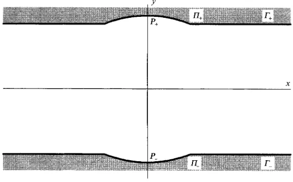
4. Further developments and generalizations

The situation considered in the two previous sections (a waveguide bounded by two parallel lines and enclosing an obstruction that is symmetric about the centreline) is not the only one in which we can rigorously prove the existence of trapped modes. Let us consider the situation illustrated by figure 3. In this case a two-dimensional wave- guide G has two symmetric indentations

P+

(we denote P =

P+

u

P-),

so that the volume

occupied by the acoustic medium 7s V = G

u

P.

The external boundaries

17= 17+

u

17- of the indentations are assumed to be piecewise smooth and parametrized in the form 17, = {(x, y ) : x = X(s), y =

k

Y(s), 0 d s d L}, where

Xi2

+

Yi2

=

1, Y(s) 2 d, Y(0) Y(L) = d, X(0) = -a, X ( L ) = a. Similarly to the conditions imposed in the beginning of $2 on the shape of the obstruction, we assume that X’(s) 2 0, (X(s), Y(s)) $:

(X($,

Y($) for all s

+

S; and Y’(s

+

0) - Y’(s - 0)

>

- 2. We shall also assume that Y(s)

+

d.

After separating out the time factor exp(iwt) we once again obtain the boundary value problem (2.1E(2.4) for a potential $(x, y), with the following slight modifications :

in (2.1) the volume occupied by the acoustic medium is V = G

u

P,

in (2.3)

a/&

Existence theorems for trapped modes 31

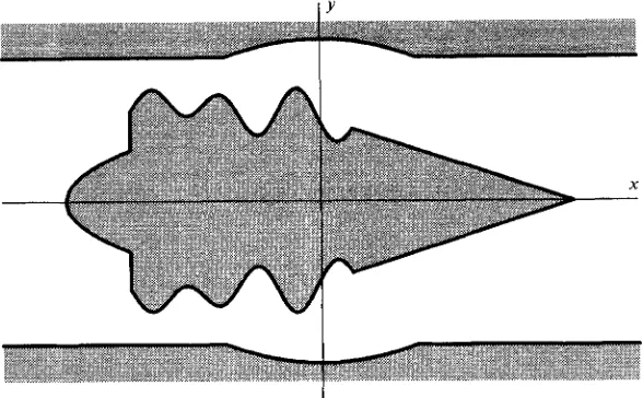
lY

FIGURE 4. Waveguide with obstruction and indentations.

Moreover, repeating practically literally the proof of Lemma 3.1 one can check that this Lemma and, consequentlx, Lemma 3.2 and Theorem 3.1 are also valid in this case. The ‘test’ function

U(x,

y ) E H,1 to be used here is very simple : for IyI

<

d it is given by

(3.2), and for IyI > d by

Y(x,y)

= 1.

It is clear that Lemmas 2.1, 2.2, 3.1, 3.2 and Theorem 3.1 also remain valid in the case when both the obstruction and the indentations (or even several different symmetric obstructions and indentations of the type described above) appear in the waveguide simultaneously (see figure

4).

M.L. appreciates the support by the Royal Society and by the Science and Engineering Research Council Grant no. H.55567.

R E F E R E N C E S

BIRMAN, M. S. & SOLOMJAK, M. Z. 1987 Spectral Theory of Self-Adjoint Operators in Hilbert Spaces. CALLAN, M., LINTON, C. M. & EVANS, D. V. 1991 Trapped modes in two-dimensional waveguides. EVANS, D. V. 1992 Trapped acoustic modes. ZMA J. Appl. Maths 49, 45-60.

EVANS, D. V. & LINTON, C. M. 1991 Trapped modes in open channels. J. FluidMech. 225,153-175. EVANS, D. V., LINTON, C. M. & URSELL, F. 1993 Trapped mode frequencies embedded in the JONES, D. S. 1953 The eigenvalues of V2u

+

hu = 0 when the boundary conditions are given on semi-

LINTON, C. M. & EVANS, D. V. 1992 Integral equations for a class of problems concerning obstacles PARKER, R. 1966 Resonance effects in water shedding from parallel plates: some experimental

PARKER, R. & STONEMAN, S . A. T. 1989 The excitation and consequences of acoustic resonances in SANCHEZ-HUBERT, J. & SANCHEZ-PALENCIA, E. 1989 Vibration and Coupling of Continuous Systems. URSELL, F. 1951 Trapping modes in the theory of surface waves. Proc. Camb. Phil. SOC. 47,347-358. URSELL, F. 1991 Trapped modes in a circular cylindrical acoustic waveguide. Proc. R. SOC. Lond.

D. Reidel.

J. Fluid Mech. 229, 51-64.

continuous spectrum. Q. J. Mech. Appl. Maths (to be published). infinite domains. Proc. Camb. Phil. Soc. 49, 668-684.

in waveguides. J. Fluid Mech. 245, 349-365.

observations. J. Sound Vib. 4, 62-72.

enclosed fluid flow around solid bodies. Proc. Inst. Mech. Engrs 203, 9-19. Springer.

A 435, 575-589.