Volume 2, No. 6, Nov-Dec 2011
International Journal of Advanced Research in Computer Science
RESEARCH PAPER
Available Online at www.ijarcs.info
Characterization of Flake Graphite Forms in Digital Microstructure Images of Gray Cast
Iron using Digital Image Analysis Techniques
Pattan Prakash*
Dept. of Computer Science and Engineering, PDA College of Engineering,
Gulbarga -585102,India [email protected]
V. D. Mytri GND College of Engineering
Bidar-585403, India [email protected]
P. S. Hiremath Dept. of Computer Science,
Gulbarga University, Gulbarga.-585106,India [email protected]
Abstract:Microstructure analysis system has an important role to play in qualitative and quantitative analysis in the gray cast iron industry. It is used to determine percent area of graphite inclusion in a given sample of gray cast iron. The ASTM A 247 standard has categorized graphite flake forms into types A, B, C, D and E. A novel method for classification and quantification of the five types of graphite flakes (lamellar), namely, type A, B, C, D and E in gray cast iron microstructure images, has been proposed. The four Haralic textural features, namely, contrast, correlation, energy and homogeneity, are employed for characterization of different flake graphite in gray cast iron. An adaptive neuro-fuzzy inference system (ANFIS) is developed for classification. The experimentation is done on actual gray cast iron microstructure images and the results are compared with the manual estimation results. The comparison indicates good correlation between manual estimation and automated estimation. Microstructure images of gray cast iron acquired from light microscope are used in the experimentation.
Keywords:ASTM A 247, gray cast iron, flake graphite, classification, Haralic texture features.
I. INTRODUCTION
In the material science, there is a strong correlation between the properties, the graphite morphology, the chemical composition, and the cooling rate. The study of microstructure images of a material provides wealth of information about the material properties [1,15]. The gray cast iron is a widely used metal alloy. The flake graphite is characteristic of gray cast iron, and components such as aluminum, carbon, and silicon promote its formation. The name gray cast iron (or gray iron) is because of the color of the fracture face. It contains 1.5-4.3% carbon and 0.3-5% silicon plus manganese, sulfur and phosphorus. It is brittle with low tensile strength, but is easy to cast. Silicon is important in making gray iron as opposed to white cast iron, because silicon is a graphite stabilizing element in cast iron, which means it helps the alloy produce graphite instead of iron carbides. Another factor affecting graphitization is the solidification rate; the slower the rate, the greater the tendency for graphite to form. A moderate cooling rate forms a more pearlitic matrix, while a slow cooling rate forms a more ferritic matrix. To achieve a fully ferritic matrix, the alloy must be annealed. Rapid cooling suppresses graphitization, partly or completely, and leads to formation of cementite, which is called white iron.
Gray cast iron has wide range of applications in metallurgy. It is used for housings where tensile strength is
non-critical, such as internal combustion engine cylinder blocks, pump housings, valve bodies, electrical boxes, and decorative castings, gears, flywheels, water pipes, engine cylinders, brake discs, gears etc. Gray cast iron's high thermal conductivity and specific heat capacity are often exploited to make cast iron cookware and disc brake rotors [1].
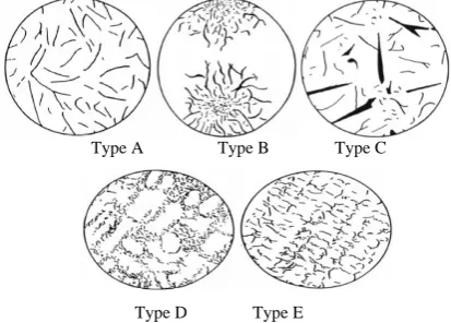
The classification and quantification of flake graphite grains is an important stage in quality control that provide vital information about the quality of the sample under inspection. The five types of graphite flake structures observed in gray cast iron are shown in the Figure 1.
Type A Type B Type C
[image:1.612.328.535.551.699.2]Type D Type E
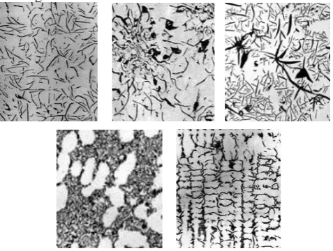
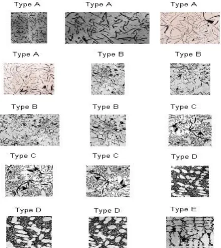
The graphite flake type A is known as Random flake graphite, the type B as Rossette flake graphite, the type C as Kish graphite, the type D as Undercooled graphite, and the type E as Interdendritic graphite. The Figure 2 shows the sample microstructure images of gray cast iron used for training.
[image:2.612.37.276.121.301.2]
Figure 2. Microstructure images of type A,B,C,D, and E .
In the manual method (visual chart inspection), the metallography expert compares each microstructure test image with the chart of five flake graphite shapes defined by ASTM A 247 committee, and classifies it accordingly. The manual method is always a challenging job. The characterization results are not consistent due to many physiological limits. In addition, the grain classification and quantification process is complicated by a number of factors; the size and shape of the grains are not constant and are found to vary from one sample to another. Hence, it is necessary to develop an digital image analysis system for classification and quantification of flake graphite forms from microstructure images.
Generally, in an automated method, the objects of interest that are present in digital microstructure images are represented by using shape features [2,4]. There are many works reported in the literature using shape features for representing graphite grains. In [10], the average grain size of super-alloy micrographs has been discussed. In [5], geometric shape features and moment variant features for classfication of graphite grains based on ISO 945 defined grains morphology are discussed. But the geometric shape features that are used for ISO 945 based graphite grain classification are not suitable for flake structures when the flake structures are in connected or in a network structure. Flake graphite classification is done in [6] using lineal intercept measurements. In this work, vertical, horizontal and circular intercept lines are super imposed on image and intercept values are determined. In gray cast iron, such flake structures are common. In [7], for gray cast iron classification, three textural features, namely, fractal dimension, roughness, and two dimension are autoregression are used with ANN classifier. In [16], bordatz texture image classification is accomplished using textural features derived from gray level co-occurence
propabilities. Although there are many featurs discussed for representation of image objects, we found that graphite morphology of gray cast iron has strong textural characteristics. Hence, the textural features are employed for representing each type of flake graphite. In the present work, Haralic textural features derived from GLCM are used. Out of twelve Haralic textural features [9], only four textural features, namely, contrast, correlation, energy and homogeneity are found to be suitable for effective classification of five types of flake graphite grains.
Classifier that is used in classification has great influence on the classification rate. The selection of classifier needs thorough experimentation. For classification, there are many classifiers in practice. Artificial neural network (ANN) based classifiers are used in [5], and fuzzy rule based classifiers in [5, 8, 12, 13, 14]. It is observed from many works in the literature that the adaptive neuro-fuzzy inference system (ANFIS) can perform better than ANN even in the case of limited training data set. This has motivated us to choose the ANFIS as classifier for automation of gray cast iron classification and quantification. With this background and motivation, we propose a novel method of automatic classification and quantification of gray cast iron using neuro-fuzzy based classification. The experimental results are compared with the manual results obtained by metallurgical experts, and the results demonstrate the efficacy of the proposed method.
A. Materials and Methods:
The proposed method is evaluated and tested on micrographs of cast iron that are obtained by using light microscope. These images are drawn from microstructure libraries [3]. The microstructure images used in testing phase are of various compositions and magnifications. In the training phase, we have used various microstructure images of each type of flake graphite images that are pre classified by metallurgical experts based on ASTM A 247 standard.
II. PROPOSED METHOD
The proposed system has two phases, namely, training and testing. The common steps in both the phases are, preprocessing, segmentation and feature extraction. The other details of the two phases are discussed in the following sections.
A. Preprocessing:
B. Feature Extraction:
In any classification system, the feature selection is a key process in object recognition and accurate classification. In the proposed system, a set of four Haralic features, out of fourteen defined features, namely, contrast, correlation, energy and homogeneity are used. Haralic features are determined using gray level co-occurrence matrix (GLCM). A GLCM is constructed with conditional-joint probabilities (Cij) of all pairwise combinations of gray levels for a fixed
window size (N), given the two parameters: interpixel distance (δ) and interpixel orientation (θ). A different GLCM is required for each (δ, θ) pair. Each GLCM is dimensioned to the number of quantized gray levels (G). A GLCM is often defined to be symmetric. The textural features are extracted through the statistical calculations applied on GLCM. These features are shift-invariant and they are defined as following:
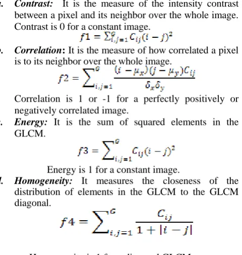
a. Contrast: It is the measure of the intensity contrast between a pixel and its neighbor over the whole image. Contrast is 0 for a constant image.
b. Correlation: It is the measure of how correlated a pixel is to its neighbor over the whole image.
Correlation is 1 or -1 for a perfectly positively or negatively correlated image.
c. Energy: It is the sum of squared elements in the GLCM.
Energy is 1 for a constant image.
d. Homogeneity: It measures the closeness of the
distribution of elements in the GLCM to the GLCM diagonal.
Homogeneity is 1 for a diagonal GLCM.
The algorithm for feature extraction from the binarized microstructure images is given in the Algorithm 1.
Algorithm 1: Feature extraction
Step 1: Input grayscale microstructure image (training image).
Step 2: Apply active contours method to the input image and obtain segmented binary image.
Step 3: Construct the GLCM1 through GLCM8 with G=2 in
eight angles (00,450,900,1350,1800, 2250, 2700, and 3150) at a distance of 1 unit.
Step 4: Compute the Haralic textural features,f1,f2,f3 and for f4 for each GLCM.
Step 5: Compute the mean values, µ1,µ2,µ3 and µ4 and
standard deviation values, SD1, SD2, SD3 and SD4
of features f1,f2,f3 and for f4, respectively.
Step 6: Repeat Steps 1 through 5 for all the known class of gray cast iron images.
Step 7: Compute µ‟1,µ‟2,µ‟3 and µ‟4, the mean values of
µ1,µ2,µ3 and µ4, respectively, of a class of images
[image:3.612.43.283.255.508.2]and tabulate these values as in the Table I.
Table I. Mean values of features of all the five flake types
Flake
type Contrast Mean Feature values of individual classes Correlation Energy Homogeneity
A 0.1045 0.6334 0.6450 0.9478
B 0.1172 0.5948 0.6084 0.9414
C 0.1923 0.5326 0.4349 0.9038
D 0.1087 0.7750 0.4205 0.9457 E
0.1302 0.6203 0.5431 0.9349
The feature vector is formed using the µ‟1,µ‟2,µ‟3 and
µ‟4
values computed in the Algorithm 1. The feature vector is used as input to ANFIS to build the Gaussian membership functions of fuzzy quantities.
C. Adaptive Neuro-Fuzzy Inference System (ANFIS):
ANFIS is one of hybrid neuro-fuzzy inference expert systems and it works as Takagi-Sugeno-type fuzzy inference system [11]. ANFIS has a similar structure to a multilayer feed forward neural network, but the links in an ANFIS only indicate the flow direction of signals between nodes and no weights are associated with the links.
D. ANFIS Structure:
ANFIS architecture consists of five layers of nodes. Out of the five layers, the first and the fourth layers consist of adaptive nodes while the second, third and fifth layers consist of fixed nodes. The adaptive nodes are associated with their respective parameters, get duly updated with each subsequent iteration while the fixed nodes are devoid of any parameters [16,17 and 18]. In general, for two-rule based system, the rules are defined as,
Rule 1: If (a is A1) and (b is B1) then (O1 = p1x +q1y + r1)
Rule 2: If (a is A2) and (b is B2) then (O2 = p2x +q2y + r2)
where x and y are the inputs, Ai and Bi are the fuzzy sets;
Oi are the outputs within the fuzzy region specified by the
[image:3.612.328.548.566.719.2]fuzzy rule; pi, qi and ri are the design parameters that are determined during the training process. The general architecture of ANFIS to implement the two if-then rules is shown in the Figure 3, in which a circle indicates a fixed node, whereas a square indicates an adaptive node.
E. Classification using ANFIS:
The ANFIS uses a strategy of hybrid approach of adaptive neuro-fuzzy inferencing and yields good classification results. The objective of classification is to classify five types of grains. The feature vectors were applied as the input to an ANFIS classifier. The ANFIS network has a total of 81 fuzzy rules and one output. The algorithm for classification of grains in a microstructure image by ANFIS is given in the Algorithm 2 and is implemented using MATLAB. The quantification of distribution of grains is also included in the algorithm after the classification step.
F. Quantification:
After classifying each type of image, the computation of the stereological parameter, namely, graphite percent area is done. This parameter is one of the essential inputs in quality control process.
Algorithm 2 : Classification and quantification
Step 1: Input grayscale microstructure image (training image).
Step 2: Apply active contours method to the input image and obtain segmented binary image.
Step 3: Construct the GLCM1 through GLCM8 with G=2
each in eight angles (00, 450, 900, 1350, 1800, 2250, 2700, and 3150) at a distance of 1 unit.
Step 4: Compute the Haralic texture features, f1,f2,f3 and for f4 for each GLCM.
Step 5: Compute the mean values, µ1,µ2,µ3 and µ4 and
standard deviation values, SD1, SD2, SD3 and SD4
of features f1,f2,f3 and for f4, respectively.
Step 6. Simulate the ANFIS with feature values computed in the Step 5.
Step 7: The output of ANFIS is the constant membership function value, which indicates the
grain class to which the microstructure in the image belongs.
Step 8: (Quantification)
Compute the stereological parameter, graphite percent area of each microstructure image.
III. EXPERIMENTALRESULTSANDDISCUSSIONS
For the purpose of experimentation, 200 digital microstructure images of each of the five flake graphite forms, namely, type A through type E are considered. The implementation is done on a Pentium 4 computer system @ 2.6 GHz using MATLAB software. In the training phase, the gray cast iron images of known type (classified by the experts) are used. These images are of size 256x256 pixels and the sample images are shown in the Figure 2. The Haralic textural features are derived from the GLCM constructed with gray levels (G=2,4,8) and eight directions (00, 450, 900, 1350, 1800, 2250, 2700, and 3150) at a distance of 1 unit. The Table I shows the mean and standard deviation values of features that are computed using the Algorithm 1.
In the testing phase, 100 microstructure images of each of the five flake forms with various resolutions and sizes are used. These images are drawn from the digital microstructure libraries [3] and these are directly taken from metal samples using optical microscope. Out of many Haralic texture features, only four textural features, which are defined in the section 2, are employed with ANFIS for classification. In the proposed system, the ANFIS is based on Takagi-Sugeno model with four inputs, one output and 81 if-then rules. The ANFIS operates with „andMethod‟ as „product‟ function and „maximize‟ as „defuzzification‟ function.
[image:4.612.320.555.293.481.2]We have conducted the ten-fold experiments for flake classification using the proposed method by varying the number of gray levels (G=2,4, 8) and the number of directions (4 and 8) and the results are shown in the Table II. The better classification results are noticed in the case of GLCM with G=2 and 8 directions. The results and the corresponding confusion matrix are shown in the Table III.
Table II. Average classification rates for each of the five flake forms.
Method
Rate of classification of five flake forms(%)
A B C D E
Proposed Method (G=2
and 8 directions) 96 98 98 97 96
Proposed Method (G=4
and 8 directions) 81.1 88.5 90 86 82
Proposed Method (G=8
and 8 directions) 80.3 85 87 85 83 Proposed Method (G=2
and 4 directions) 82.1 88 92.2 88 86
Proposed Method (G=4
and 4 directions) 79 89 89 84 80
Proposed Method (G=8
and 4 directions) 75 74 79 79.5 77
Manual (by experts) 90.6 92 92 91 91
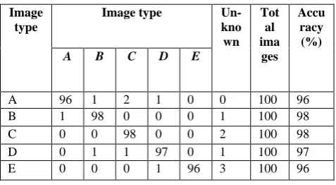
Table III. Confusion matrix for classification of the five forms of flake graphite images using proposed method (G=2 and 8 directions).
Image type
Image type Un-
kno wn
Tot al ima ges
Accu racy (%) A B C D E
A 96 1 2 1 0 0 100 96
B 1 98 0 0 0 1 100 98
C 0 0 98 0 0 2 100 98
D 0 1 1 97 0 1 100 97
E 0 0 0 1 96 3 100 96
[image:4.612.320.559.509.640.2]Figure 4. Sample images of the classification results.
The Table II shows the comparison of the classification rate of the proposed method with the manual results obtained by metallurgical experts. The variations of microstructures are in terms of image magnifications, orientations and quality. The quantification of the graphite flakes in terms of the stereological parameter, namely, graphite percent area, which is practically the main factor in quality control, is determined. This process comprises of the count of pixels that correspond to graphite flakes in samples. The distribution of graphite area (%) for flakes of type A,B,C,D and E is shown in the Figure 5. It is observed that the results obtained by the proposed method is in close agreement with the manual results obtained by the metallurgical expert.
Figure 5. Distribution of graphite area (%) for flakes of type A,B,C,D and E.
IV. CONCLUSION
In this paper, we have proposed an automated system for classification and quantification of graphite flake in gray cast iron. The experimental results are compared with the manual results obtained by metallurgy expert. The proposed method based on the Haralic textural features and the adaptive neuro-fuzzy inference system yields better classification rates. The adaptive neuro-fuzzy logic addresses such applications perfectly as it resembles human decision making with an ability to generate precise solutions from certain or approximate information. The results demonstrate that the proposed system is efficient. The ANFIS permits use of incremental changes in the training dataset and the system learns adaptively.
V. REFERENCES
[1]. Handbook Committee, Hand book of ASM International, Vol 9, Metallography and Microstructures, ISBN:0-87170-706-3. [2]. Milan Sonka, Vaclav Hlavac, Roger Boyle, “Image
Processing, Analysis, and Machine Vision”, 2e. PWS Publishing, ISBN:81-315-0300-3, ISSN:978-81-315-0300-3, 1999.
[3]. Microstructures libraries: http://www.metalograf.de/start-eng.htm, www.doitpoms.ac.uk
[4]. G. Vander Voort Website: http://georgevandervoort.com
[5]. Pattan Prakash, V.D.Mytri and P.S.Hiremath, “Classification of Cast Iron Based on Graphite Grain Morphology using Neural Network Approach”, Proc. of SPIE Vol 7546, Second Inter National conference on Digital Image Processing 2010 (ICDIP 2010), Singapore, Feb 26- 28, pp 1 – 75462S-6, 2010.
[6]. G.M. Lucas, T.P. Weber, and L.Barnard, “Characterization of Flake Graphite Forms in Gray Iron through Image Analysis”, J. Microsc Microanal, Vol 14, Issue 2, p 582, Jan 2008
[7]. Hong Jiang , Yiyong Tan, Junfeng Lei, Libo Zeng Zelan Zhang & Jiming Hu, “Auto-analysis system for graphite morphology of gray cast iron”, J. of Automated methods and management in chemistry”, vol 25, no.4, pp 87-92, June-July 2003.
[8]. E.H. Mamdani and Assilian, “An Experiment in Linguistic Synthesis with a Fuzzy Logic Controller”, Intl. Journal on Man-Machine Studies, Vol 7, pp 1-13,1975.
[9]. Haralick, R.M., K. Shanmugan, and I. Dinstein, "Textural Features for Image Classification", IEEE Transactions on Systems, Man, and Cybernetics, Vol. SMC-3, 1973, pp. 610-621.
[10].Wanda Benesova, Alfred Rinnhofer, Gerhard Jacob, “Determining The Average Grain Size of Super-Alloy Micrographs”, Proceedings of IEEE International conference on Image Processing (ICIP 2006), pp:2749-2752,2006.
[image:5.612.40.284.506.697.2][12].T.M. Nazmy, H. El-Messiry, B. Al-Bokhity, “Adaptive Neuro-Fuzzy Inference System for Classification of ECG Signals, J. of Theoretical and Applied Information Technology”, Vol 12, pp. 71-76, 2009.
[13].Dhaval Mehta, E.S.V.N.L. Diwakar and C.V. Jawahar, “A rule-based Approach to Image Retrieval”, Proc. of IEEE Conf. on Convergent Technologies (IEEE TENCON), Bangalore, India, pp 71-76,2003.
[14].Kulkarni,S.,Verma, B.,Sharma,P. and Selvaraj,H. Content Based Image Retrieval using a Neuro-Fuzzy Technique. Proc.
Intl., Joint Conf. Neural Networks (IJCNN‟99), Washington DC, USA, July, pp 846-850, 1999.
[15].L.Wojnar, Image Analysis, Applications in Materials Engineering, CRC Press,1999.
[16].Hong-Choon Ong, Hee-Kooi Khoo, “Improved Image Texture Classification using Gray Level Co-occurrence Probabilities with Support Vector Machines Post-processing”, European Journal of Scientific Research, Vol. 36, No. 1,pp 56-64, 2009. [17].Tony F. Chan, Luminita A. Vese, “Active Contours without