Influences Combination of Multi Sensor Images on Classification Accuracy

(1)

Volume 4, No. 9, July-August 2013

International Journal of Advanced Research in Computer Science

RESEARCH PAPER

Available Online at www.ijarcs.info

ISSN No. 0976-5697

Influences Combination of Multi-Sensor Images on Classification Accuracy

Firouz Abdullah Al-Wassai*

Research Student, Dept. of Computer Science (SRTMU), Nanded, India

Abstract: This paper focuses on two main issues; first one is the impact of combination of multi-sensor images on the supervised learning classification accuracy using segment Fusion (SF). The second issue attempts to undertake the study of supervised machine learning classification technique of remote sensing images by using four classifiers like Parallelepiped (Pp), Mahalanobis Distance (MD), Maximum-Likelihood (ML) and Euclidean Distance(ED) classifiers, and their accuracies have been evaluated on their respected classification to choose the best technique for classification of remote sensing images. QuickBird multispectral data (MS) and panchromatic data (PAN) have been used in this study to demonstrate the enhancement and accuracy assessment of fused image over the original images using ALwassaiProcess software. According to experimental result of this study, is that the test results indicate the supervised classification results of fusion image, which generated better than the MS did. As well as the result with Euclidean classifier is robust and provides better results than the other classifiers do, despite of the popular belief that the maximum-likelihood classifier is the most accurate classifier.

Keywords: Segment Fusion, Euclidean Classifier, Mahalanobis Classifier, Parallelepiped Classifier, Maximum-Likelihood, Classification.

I. INTRODUCTION

The classification is defined as information of extracting process that analyses the adopted spectral signatures by using a classifier and then assigns the spectral vector of pixels to categories according to their spectral. Depending on the level of pattern classification procedure techniques are used in classifying images can be broadly categorized as either supervised or unsupervised. In the case of unsupervised classification means by which pixels in the image are assigned to spectral classes without the user having foreknowledge of training samples or a-prior knowledge of the area. While In the case of supervised classification, it requires the user provide the types of cover sets in the image e.g., water, cobble, deciduous forest, etc. As well as a training field for each cover type. The training field typically corresponds to an area in the image, which has contains of the cover type, and the collection of all training fields is known as the training set or ground-truth data. These training set can be obtained using site visits, maps, aerial photographs or even a photo interpretation of a colour composite product formed from the satellite image data [1].

The ground-truth data is then used to assign each pixel to its most probable cover type. Many factors in every case, the crucial steps are: (i) selection of a set of features which describes the best pattern from the original feature set and thus can be viewed as a principal pre-processing tool prior to solving classification problems [2], (ii) choice of a suitable classifier for the comparison of the pattern describing the object to be classified and the target patterns and (iii) a third stage, that of assessing the degree of accuracy of the allocation process. Many factors affect the accuracy of image classification and the quality of land cover maps, which is often perceived as being insufficient for operational use [3-4]. Classification accuracy is a function of training set selection, and a good training set has the following characteristics [5]:1). It should contain samples describing all classes,2) It should have a sufficient number of independent samples for each class, and 3) It should be made up of samples that completely describe the intra-class variability.

The feature-selection techniques that are most widely used in remote sensing generally require the definition of a discriminant function and a decision rule. The decision rule is a measure of the effectiveness of the considered subset of features, and the discriminant function is an algorithm that aims at efficiently finding a solution (i.e., a subset of features) that optimizes the adopted decision rule. In standard feature-selection methods, several feature-feature-selection algorithms have been proposed for selecting of training set, e.g., [6, 1]. the discriminant functions typically adopted are statistical measures that assess the separability of the different classes on a given training set but do not explicitly take into account the stationarity of the features (e.g., the variability of the spectral signature of the land-cover classes) [ 7]. This approach may result in selecting a subset of features that retains very good discrimination properties in the portion of the scene close to the training pixels (and therefore with similar behavior), but are not appropriate to model the class distributions in separate portions on the scene, which may present different spectral behavior[8]. In general, Current image processing techniques are limited in their ability to automatically extract accurate land cover features [9].

(2)

Section 2 describes the basic terms in supervised image classification; Section 3 describes the supervised image classification methods; section 4 presents the data sets that used in the experimental analysis and classification results of fused image and Section 5 conclusions. All of the image classification speeds have been calculated, that using the same training data for each image test. The computer hardware used to record the image classification algorithm speeds are an Intel® Core ™ i5-245OM CPU@ 2.50 GHz with Turbo Boost 3.10 GHz and 4.00GB RAM installed. The ALwassaiProcess software was running on operating system Microsoft Windows 7 64-bit respectively.

II. BASICTERMSINSUPERVISEDIMAGE CLASSIFICATION

In this section we would explain some basic terms about supervised image classification in general. A digital image is composed by pixels or points, and these points usually represent values in a multidimensional space. Each point can be represented as:

Where is the value of pixel in the band or feature (the term feature is more used since band is more related with spectral bands). The vector is also called the feature vector or measurement vector. Feature Space is the set of all possible feature vectors. Usually the value of a pixel in a band is the brightness or gray level for that pixel, but for some classification tasks one may want to use other features, for example, texture measures, etc. In this case it would be necessary to normalize the values in the feature space so all feature space dimensions will be the same.

Classification is a method by which unique labels are assigned to pixels based on the values of the vector . This decision is made by applying a discriminant function associated with class to vector , and choosing the largest . In other words: for all classes in a classification task the pixel is classified as class if its

is the largest value for all , or:

(1.1) The total number of classes in supervised classification is determined by the nature of the problem and by user's decision. The discriminant function depends on the chosen classification method. Some discriminant functions used in the different classifiers in this ALwassaiProcess software will be presented. Classification can also be considered as the partition of the feature space in mutually exclusive parts. Pixels are assigned to classes based on this partition.

Here is a little more formal definition of the above, which is known as Bayesian Classifier, The classes in a classification task can be denoted by:

Where is the total number of classes and the probability that the correct class for is is given by:

Where is called the a-posteriori probability. To decide which class is the best (or has the least classification error) for the pixel we should select the largest on other words, select from between the

probabilities that the correct class for pixel is for all the highest one, or [17]:

(1.2) The problem is that these we need to determine the class for pixel are unknown. If we have enough samples from all classes we can estimate the probability for finding a pixel from class in position , denoted by

. If there are classes, there will be also values for denoting the relative probabilities that the pixel belongs to the class . The relation between and

is given by Bayes' theorem [17]:

Where is the probability that class occurs in the image. Also called a-priori probability and is the probability of finding a pixel from any class at position . By comparison the ) are posterior probabilities. Using (1.2) it can be seen that the classification rule of (1.1) is [17]:

Where is the natural logarithm, so that (1.3) is restated as [17]:

(1.5) Where the discriminant function and is calculated differently for the different classification schemes. When is not available it is considered as equal to 1 for all classes.

III. SUPERVISEDIMAGECLASSIFICATION METHODS

This study implied different discriminant functions considered as the classification strategy and will be used to classifier the training set from each of the defined classes as below. In the following different discriminant functions the training data will be extracted by having certain regions and they will have their RGB values represented by the mean red, the mean blue and the mean green values separately. Supposing the mean vector is a n-dimension vector, where n is the number of features (or image bands). The mean vector for class is calculated for each feature as:

Where is the number of samples and is the jth sample

A. Parallelepiped Classifier (Pp) :

(3)

An example illustrating the specification of the topology of a Pp classifier in the case of a two-dimensional feature space is shown in Fig. 1.

Fig. 1: Pp Classifier Example

B. Mahalanobis Distance Classifier (MD):

Classification is performed on MD classifier from each pixel to the signatures centers. Basically the classifier assigns class to pixel if:

The discriminant function for the Mahalanobis distance classifier is as follows [19-20]:

= (1.6)

Where is the MD classifier for class . and are the mean vector and the inverse covariance matrix for the data of class . For a MD classifier signature we need some of the components shown in equation 1.6: the classes' mean and inverse of the covariance matrix . The data will be stored in separate planes in the depth direction, one for the mean and one for the inverse of the covariance matrix. The classification is done by choosing the lowest

for all class .

C. Maximum-Likelihood Classifier (ML):

The ML classifier assumes that the classes are unimodal and normally distributed. Its discriminant function is given by [19]:

(1.7)

Often the analyst has no useful information about the in which case a situation of equal prior probabilities is assumed; as a result can be removed from (1.7) since it is then the same for all . In that case the 1/2 common factor can also be removed leaving, as the discriminant function [19]:

(1.8)

Implementation of the ML decision rule involves using either (1.7) or (1.8) in (1.5). For a ML classifier signature we need some of the components shown in equation 1.8: the classes' mean vector and inverse of the covariance matrix . To help with the analysis of the signature's distributions and speed calculation of the likelihoods, the covariance matrix and the negative of the logarithm of its determinate will also be stored in the signature. The data will be stored in separate planes in the depth direction, one for the mean, one for the covariance matrix, one for the inverse of the covariance matrix and one for the negative logarithm of the determinate of the covariance matrix. The classification is done by choosing the maximum for all class . N is the number of features in the image.

D. Euclidean Distance Classifier (ED):

The ED is a particular case of Minkowski sometimes is also called Quadratic Mean. Classification is performed on ED classifier from each pixel to the signatures centers. Basically the classifier assigns class to pixel if:

The discriminant function for the EC classifier takes the following form and has the unit circle detailed in [21]:

(1.9)

IV. EXPERIMENTALRESULTS

A. Test data sets:

(4)

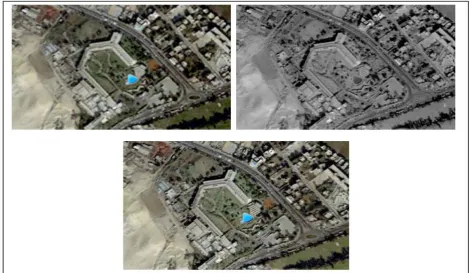
Figure. 2: Experimental Test Images over the Pyramid Area of Egypt in 2002. Quickbird Data MS and Quickbird PAN, Image Fused Resulted By SF Algorithm.

B. Supervised Image Classifiers:

In the supervised classification, the acquisition of ground truth data for training and assessment is a critical component in process. In the study the developed system was designed to extract the training data test by having certain regions selected as decried below. The classification consists of the following steps:

a. Step 1: Select the number and the size of regions that will be the training data the image as shown in Fig.3. The author has selected twelve classes as shown in Fig.4, and the size of each region selecting for the training data is 4 × 4 pixels was chosen.

b. Step 2: Experts the Image; Experts training data; and Select discriminant function as shown in Fig.5.

c. Step 3: apply the decision rule between the pixels in the image and every reference class according to the selected discriminant function as shown in Fig.6. d. Step 4: Assign each pixel to the reference class that

has the decision rule between pixel and reference class then stored in separate planes in the depth direction.

e. Step 5: selected different five regions of each reference class for the accuracy assessment of image classification as shown in Fig.7

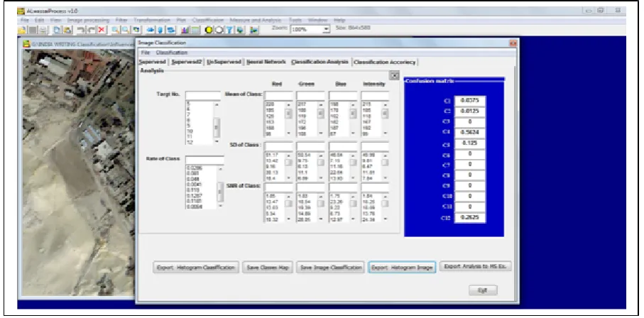
f. Step 5: The Accuracy Assessment of Image Classification as shown in Fig.8.

(5)

Figure.5: Illustrate Step 2: the Automatic Classification Process: Experts The Image; Experts Training Data; And Select Classifier Methods.

Figure.6: Illustrate Step 3: Apply The Decision Rule Between The Pixels In The Image And Every Reference Class According To The Selected Discriminant Function.

(6)

Figure 8: Illustrate Step 5: The Accuracy Assessment Of Image Classification.

C. Classification Results Of Fused Image:

To evaluate the performance of the proposed active learning strategies the four classifiers were applied for both MS QuickBird and fusion data after the fusion process. To the description of classification error, it is necessary to configure the error matrix and decide the measurements. Generally, there are descriptive statistic and analytic statistic from the error matrix. Overall accuracy, producer’s accuracy (omission error) and user’s accuracy (commission error) as well as Kappa statistic belong to descriptive statistic. In this study, as limited time, we focus the accuracy assessment of image classification only on the Overall accuracy for fused image. For such purpose, we first selected different five regions that have a 4×4 size for each reference class set is shown above in Fig.4. Table (1- 4) and Table (5-8) list the error matrix for both classified results, respectively. The overall measured accuracies of the Pp, MD, ML and ED classifiers for MS were 59.735%; 64.60%; 59.108% and 87.257% respectively, and for fused image classified results were 63.498%; 60.838%; 58.363 % and 91.476% respectively. Fig. 9 show the classified results for fusion image and MS QuickBird image by the four classifiers.

The Pp classifier is quick and easy to implement but the classification results has error, because some pixels lie inside more than one Pp or outside all Pps, therefore a pixel

in those regions not classified. The classification results of the ML and MD classifiers are not surprising when we consider the fact that both ML and MD classifiers use class variances in each spectral band for calculating distances for classification. Both MD and ML classifiers use parametric rules that require normally distributed data and well defined variances for image data and each training class, while most image data do not show normal distribution, and most of the training classes have high variances of pixel values in each band. The ML and MD classifiers rules can be quite diagnostic in distinguishing different features with image data that show normal distribution and have well defined variances in each spectral band for each surface object. However, when those assumptions are violated, their performances are less than desirable. Classification accuracy results of the supervised ED classifier are presented in Table 8 with the overall accuracy of 91.476percent. The mapping result of the ED classifier shows much higher overall accuracy of 91.476 % compared to that of the ML classifier (58.363 %) or MD classifier (60.838%) and Pp classifier (63.498%). In general, the supervised classification results of fusion image generated better than did the MS QuickBird. The best results overall accuracies with ED classifier than the other did.

Table (1): Error Matrix for MS QuickBird Classified Result By Pp Classifier

C1 C2 C3 C4 C5 C6 C7 C8 C9 C10 C11 C12 R. Total

C1 0.6999 0.1 0.0625 0.1375 0.9999

C2 0.4499 0.1625 0.3874 0.9998

C3 0.3624 0.5124 0.125 0.9998

C4 0.1093 0.2343 0.6093 0.0156 0.0312 0.9997

C5 0.0375 0.9624 0.9999

C6 0.2874 0.6124 0.075 0.025 0.9998

C7 0.0125 0.0125 0.9749 0.9999

C8 0.0222 0.0444 0.2222 0.0888 0.6222 0.9998

C9 0.9999 0.9999

C10 0.3249 0.075 0.125 0.3499 0.125 0.9998

C11 0.2 0.0125 0.25 0.2 0.3374 0.9999

C12 0.0375 0.0125 0.5624 0.125 0.2625 0.9999

C.Total 2.0811 0.8092 0.8499 1.4411 2.0345 0.8387 1.4154 0.6222 1.0249 0.25 0.3686 0.2625 11.9981

(7)

Table (2): Error Matrix for MS QuickBird Classified Result By MD Classifier

C1 0.6874 0.3124 0.9998

C2 0.1 0.8999 0.9999

C3 0.7624 0.15 0.0875 0.9999

C4 0.3906 0.5937 0.0156 0.9999

C5 0.9999 0.9999

C6 0.9999 0.9999

C7 0.0125 0.9874 0.9999

C8 0.4 0.6 1

C9 0.9999 0.9999

C10 0.2125 0.1125 0.05 0.6249 0.9999

C11 0.5999 0.3999 0.9998

C12 0.025 0.7749 0.2 0.9999

C.Total 0.6874 0.1 0.9749 0.4156 4.7307 1.1249 1.1249 0.6 0.9999 0.6249 0.4155 0.2 11.9987

Overall accuracy 0.6874 0.1 0.7624 0.3906 0.9999 0.9999 0.9874 0.6 0.9999 0.6249 0.3999 0.2 0.646025

Table (3): Error Matrix for MS QuickBird Classified Result By ML Classifier

C1 0.15 0.8499 0.9999

C2 0.0125 0.9874 0.9999

C3 0.7499 0.15 0.1 0.9999

C4 0.3437 0.5 0.1562 0.9999

C5 0.9999 0.9999

C6 0.9999 0.9999

C7 0.9999 0.9999

C8 0.4 0.6 1

C9 0.9999 0.9999

C10 0.1875 0.1 0.075 0.6374 0.9999

C11 0.5999 0.3999 0.9998

C12 0.025 0.7749 0.2 0.9999

C.Total 0.15 0.0125 0.9374 0.7687 4.862 1.0999 1.1749 0.6 0.9999 0.6374 0.5561 0.2 11.9988

Table (4): Error Matrix for MS QuickBird Classified Result By ED Classifier

Euclidian C1 C2 C3 C4 C5 C6 C7 C8 C9 C10 C11 C12 R. Total

C1 0.9749 0.025 0.9999

C2 0.0375 0.7874 0.1625 0.0125 0.9999

C3 0.9999 0.9999

C4 0.0781 0.9218 0.9999

C5 0.25 0.05 0.6999 0.9999

C6 0.8999 0.1 0.9999

C7 0.9999 0.9999

C8 1 1

C9 0.9624 0.0375 0.9999

C10 0.2874 0.7124 0.9998

C11 0.0375 0.0375 0.2125 0.025 0.6874 0.9999

C12 0.0125 0.0375 0.0875 0.0375 0.8249 0.9999

Total 1.0624 1.0749 1.6154 1.0593 0.9249 0.8999 0.9999 1 0.9624 0.7749 0.7999 0.8249 11.9988

overall accuracy 0.9749 0.7874 0.9999 0.9218 0.6999 0.8999 0.9999 1 0.9624 0.7124 0.6874 0.8249 0.872566667

Table (5): Error Matrix Classified Result for Fusion Image By Pp Classifier

C1 0.9749 0.025 0.9999

C2 0.025 0.5249 0.0625 0.3249 0.0625 0.9998

C3 0.125 0.8624 0.0125 0.9999

C4 0.5 0.0312 0.3125 0.0312 0.0937 0.0312 0.9998

C5 0.3124 0.0125 0.6499 0.025 0.9998

C6 0.0375 0.8124 0.025 0.125 0.9999

C7 0.0125 0.125 0.8624 0.9999

C8 0.1555 0.2444 0.1333 0.0222 0.4444 0.9998

C9 0.9999 0.9999

C10 0.2874 0.2375 0.1625 0.3124 0.9998

C11 0.1625 0.075 0.1125 0.0375 0.0125 0.0125 0.5499 0.0375 0.9999

C12 0.05 0.025 0.0375 0.0125 0.175 0.075 0.6249 0.9999

C.Total 1.7803 1.4623 1.3311 0.4 1.4629 1.1124 0.9936 0.1333 1.0221 0.4499 0.7436 1.1068 11.9983

(8)

Table (6): Error Matrix Classified Result for Fusion Image By MD classifier

C1 0.5874 0.3374 0.075 0.9998

C2 0.0875 0.4749 0.4374 0.9998

C3 0.4749 0.3624 0.1625 0.9998

C4 0.25 0.0156 0.0625 0.2031 0.4687 0.9999

C5 0.9624 0.0125 0.025 0.9999

C6 0.15 0.8499 0.9999

C7 0.2625 0.6249 0.1125 0.9999

C8 0.2888 0.7111 0.9999

C9 0.9999 0.9999

C10 0.9999 0.9999

C11 0.0125 0.0625 0.9249 0.9999

C12 0.0125 0.0125 0.025 0.9499 0.9999

C. Total 0.5874 0.0875 0.4749 0.2625 1.8028 0.4125 0.6249 0.2888 0.9999 2.4622 1.7654 2.2297 11.9985

Table (7): Error Matrix Classified Result for Fusion Image By ML Classifier

C1 0.3999 0.4374 0.1625 0.9998

C2 0.0875 0.4499 0.4624 0.9998

C3 0.4624 0.3624 0.175 0.9998

C4 0.2031 0.0468 0.0781 0.6718 0.9998

C5 0.9249 0.0375 0.0375 0.9999

C6 0.1125 0.8874 0.9999

C7 0.2 0.6249 0.175 0.9999

C8 0.2888 0.7111 0.9999

C9 0.9999 0.9999

C10 0.9999 0.9999

C11 0.0625 0.9374 0.9999

C12 0.0125 0.025 0.9624 0.9999

Column total 0.3999 0.0875 0.4624 0.2031 1.8122 0.3125 0.6249 0.2888 0.9999 2.5465 1.7154 2.5453 11.9984

Table (8): Error Matrix Classified Result for Fusion Image By ED Classifier

C1 0.9624 0.025 0.0125 0.9999

C2 0.8749 0.1 0.025 0.9999

C3 0.9999 0.9999

C4 0.1093 0.8906 0.9999

C5 0.1 0.8999 0.9999

C6 0.9499 0.05 0.9999

C7 0.9999 0.9999

C8 1 1

C9 0.9999 0.9999

C10 0.2375 0.7624 0.9999

C11 0.1625 0.8374 0.9999

C12 0.2 0.7999 0.9999

C total 0.9624 0.9999 1.5092 1.0906 1.0124 0.9499 0.9999 1 0.9999 0.8124 0.8624 0.7999 11.9989

(9)

Figure.9: The Left Side Classified Result Of MS Quickbird And The Right Side kClassified Result Of Fusion Image With Color Code Of Each Land Class By: (a) Pp Classifier (b) MD classifier; (c) ML Classifier; (d) ED Classifier.

V. CONCLUSION

In the study there are four supervised classifications are introduced as the following: Pp, MD, ML and ED classifiers. The supervised classification of the MS QuickBird Classified image has the lowest accuracy in comparison of the Fused Image Classified Result. When two data sets combined together (MS and PAN images) by using the SF algorithm in feature-level image fusion, confusion, problem was solved effectively. Another advantage of

feature-level image fusion is its ability to deal with ignorance and missing information.

The MD classifier produced results very similar to that of the ML classifier and they have the least accurate of all according to experimental result of this study. Because they use a parametric rule that requires data normal distribution and well defined covariance’s for each band in image data and each training class. Out of all four supervised classifiers ED Classifier generate more accurate classification results than other classifiers do, despite the popular belief that the ML classifier is the most accurate classifier.

(a) PpClassifier

(b) MD Classifier

(c) ML Classifier

(10)

VI. ACKNOWLEDGMENT

The authors would like to thank DigitalGlobe for providing the data sets used in this paper.

VII. REFERENCES

[1] Gupta S., Rajan K. S., 2011. “Extraction of training samples from time-series MODIS imagery and its utility for land cover classification”. International Journal of Remote Sensing Vol. 32, No. 24, pp. 9397–9413

[2] Wang X., Yang J., Teng X., Xia W.,Jensen R., 2007. “Feature selection based on rough sets and particle swarm optimization”. Pattern Recognition Letters 28 (2007), no. 4, 459-471.

[3] Foody GM., 2002, “Status of land cover classification accuracy assessment”. Remote Sensing of Environment, vol. 80, pp. 185-201.

[4] Lu D., Weng Q., 2007, “A survey of image classification methods and techniques for improving classification performance”. International Journal of Remote Sensing, vol. 28, pp. 823-870.

[5] Marf M., Bruzzone L.,Vails, G., 2007, “A support vector domain description approach to supervised classification of remote sensing images”. IEEE Transactions on Geoscience and Remote Sensing, 45, pp. 2683–2692.

[6] Guo B., Damper R. I., Gunn S. R., Nelson J. D. B., 2008. “A fast separability-based feature-selection method for high-dimensional remotely sensed image classification,” Pattern Recognit., Vol. 41, No. 5, pp. 1653–1662.

[7] Baraldi A., Wassenaar T., Kay S., 2010. “Operational performance of an automatic preliminary spectral rule-based decision-tree classifier of spaceborne very high resolution optical images,” IEEE Trans. Geosci. Remote Sens., vol. 48, no. 9, pp. 3482–3502.

[8] Lorenzo B., Claudio P., 2009. “A Novel Approach to the Selection of Spatially Invariant Features for the Classification of Hyperspectral Images With Improved Generalization Capability,” IEEE Trans. Geosci. Remote Sens., Vol. 47, No. 9, pp. 3180 - 3191.

[9] Baraldi A., Durieux L., Simonetti D., Conchedda G., Holecz F., Blonda P., 2010. “Automatic Spectral Rule-Based Preliminary Classification of Radiometrically Calibrated SPOT-4/-5/IRS, AVHRR/MSG, AATSR, IKONOS/ QuickBird/ OrbView/ GeoEye, and DMC/SPOT-1/-2 Imagery-Part I: System design and implementation”, IEEE Transactions on Geoscience and Remote Sensing, vol. 48, No. 3, pp. 1299-1325.

[10] Al-Wassai F. A., N.V. Kalyankar, A. A. Al-zuky, 2011. “Feature-Level Based Image Fusion Of Multisensory Images”. International Journal of Software Engineering Research & Practices, Vol.1, No. 4, pp. 8-16.

[11] Al-Wassai F. A., N.V. Kalyankar, 1012. "A Novel Metric Approach Evaluation for the Spatial Enhancement of Pan-Sharpened Images". International Conference of Advanced

Computer Science & Information Technology, 2012 (CS & IT), 2(3), 479 – 493. DOI : 10.5121/ csit.2012.2347.

[12] Al-Wassai F. A., N.V. Kalyankar, 1012. “The Segmentation Fusion Method On10 Multi-Sensors”. International Journal of Latest Technology in Engineering, Management & Applied Science, Vol. I, No. V ,pp. 124- 138.

[13] Al-Wassai F. A., N.V. Kalyankar, A. A. Al-Zaky, "Spatial and Spectral Quality Evaluation Based on Edges Regions of Satellite: Image Fusion". 2nd International Conference on Advanced Computing & Communication Technologies ACCT 2012, presiding in IEEE Computer Society, pp. 265-275. DOI:10.1109/ACCT.2012.107.

[14] Al-Wassai F. A., N.V. Kalyankar, A. A. Al-zuky, 2011. “Studying Satellite Image Quality Based on the Fusion Techniques”. International Journal of Advanced Research in Computer Science, 2011, Volume 2, No. 5, pp. 516- 524.

[15] Firouz A. Al-Wassai, N.V. Kalyankar, A. A. Al-zuky, 2011. “Multisensor Images Fusion Based on Feature”. International Journal of Advanced Research in Computer Science, Volume 2, No. 4, July-August 2011, pp. 354 – 362.

[16] Al-Wassai F. A., N.V. Kalyankar, A. A. Zaky, 2012."Spatial and Spectral Quality Evaluation Based on Edges Regions of Satellite: Image Fusion”, IEEE Computer Society, 2012 Second International Conference on ACCT 2012, pp.265-275.

[17] Richards J. A., and Jia X., 1999. “Remote Sensing Digital Image Analysis”. 3rd Edition. Springer - verlag Berlin Heidelberg New York.

[18] Schowengerdt R. A.,2007. “Remote Sensing: Models and Methods for Image Processing”. 3rd Edition, Elsevier Inc.

[19] Tso b. and Mather P. M., 2009 “Classification Methods for Remotely Sensed Data”. 2nd Edition, Taylor & Francis Group, LLC.

[20] Tala A. Al-Khateeb ,2008.“Land Use Classification Utilizing Landsat Thermal Band - Based on Wavelet Transform”. Eng.&Tech.Vol.26.No.11,2008.

[21] Zezula P., Amato G., Dohnal V., Batko M., 2005. Similarity Search: The Metric Space Approach”. Advances in database systems, Springer, New York.

Short Bio Data for the Authors

Firouz Abdullah Al-Wassai received her B.Sc. degree in Physics in 1993from University of Sana’a, Yemen, Sana’a and M.Sc.degree in Physics in 2003from Bagdad University, Iraq. Currently she is Research student PhD in the department of computer science (S.R.T.M.U), Nanded, India. She has published papers in twelve International Journals and conference.

(11)

from Dr. B.A.M.U, Aurangabad. In 1980 he joined as a leturer in department of physics at Yeshwant Mahavidyalaya, Nanded. In 1984 he completed his DHE. He completed his Ph.D. from Dr.B.A.M.U. Aurangabad in 1995. From 2003 he is working as a Principal to till date in Yeshwant Mahavidyalaya, Nanded. He is also research guide for Physics and Computer Science in S.R.T.M.U, Nanded. 03 research students are successfully awarded Ph.D in Computer Science under his guidance. 12 research students are successfully awarded M.Phil in Computer Science under his guidance He is also worked on various boides in S.R.T.M.U, Nanded. He is also worked on various