DOI: http://dx.doi.org/10.26483/ijarcs.v8i8.4671
Volume 8, No. 8, September-October 2017
International Journal of Advanced Research in Computer Science
RESEARCH PAPER
Available Online at www.ijarcs.info
ISSN No. 0976-5697
DETERMINING LOWEST COST COMMUNICATION PATH IN DISTRIBUTED
DATABASE SYSTEM
Rakesh Kumar Pandey
Research Scholar
University Department of Statistics and Computer Applications,
T. M. Bhagalpur University, Bhagalpur-812007, India
Dr. Sachindra Kumar Azad
*Associate Professor and Head
University Department of Statistics and Computer Applications,
T. M. Bhagalpur University, Bhagalpur-812007, India
Abstract: Relational Database is interpreted as collection of interrelated data or records, where Database Management System is software of synthesize programs used to manage overall problem arises in the Relational database system. Join Operation is used to combine more than one relation using single query statement. Sometimes, it is impossible to get result from a single relation of the relational database in their case join operation is useful to fetch data from more than one relation of the database. Join is a performed as Cartesian product followed by some specific condition process. In this paper we are going to proposed, an algorithm that reduce the communication cost when the join operation is performed on the distributed database query system. In distributed database system, join operation is performed on different sites of the communication network. This proposed algorithm is automatically selecting the lowest cost communication path to perform the join operation on relational database.
Keywords: Join, Relational Database, Normalization, Key, Cross join, DDMS
I. INTRODUCTION
In Relational database data model [E.F. Codd 1970, 1972] design, the join operation is one the most important concept to fetch related tuple from different relation of the database into single tuple under some specific condition. During database designing the designer of the database decomposed the relation into several small relations to achieve the higher normal form. Decomposition is the operation of breaking down a huge relation of the database into sub parts [1]. The main aim of decomposition is to replaces a huge relation with a collection of various smaller relations. It breaks the relation into multiple relations in a database. Decomposition always should be lossless, because it confirms that the records in the master relation can be accurately redesigned using the concept of join on the decomposed relations [2]. If decomposition is not done correctly on the relation, then it may lead to problems like loss of data. While normalizing a relation in a relational database system the results come out in related information that being saved in different relations of the database. Hence, SQL queries that require data from different relation are very familiar. To satisfy the queries join operation is to be introduced [3]. In other hand a join can be expressed as a cross-product of two or more relations followed by selections and projections operation in Relational Algebra, joins appear much easier in practice than simple cross-products. Further, the result of a cross-product is generally contains more number of tuple than the result of a join, and it is much more important to understand joins and implement them without cross-product [4]. Only For these reasons, joins operations have received a lot of observations, and there were many variants of the relational database join operations. This paper collates all the information present in the literature in order to study the new and common features of join operations [5]. With this data, it
is possible to classify the join operations into different categories. The different categorizations scheme and different
approaches to implement join processing are provided in this paper. Relational database join operations are categorized into two-way and multi way scheme [6]. Join operations is considered as two-way, when it is executed on two relations of database and multi way when more than
two relations of database are joined together. A multiway join gives the same result as a two way joins series gives [7]. A join between m numbers of relations is generally executed as the sequence on n−1 two-way joins in database [Mackert and Lohman, 1986].
pure distributed database management system environment [12]. The Most commonly replication is used to enhanced the local host relational database table’s performance and provide the security, because another way to access tuples are also exists in the database query [13]. For Example, the application programs which are stand alone are normally use the local database system to store tuples in the tuples. While we are using some applications programs that are use to access the database which are stored in the remote site database, to access this type of database may increase the communication cost and also maximize the network traffic but other database servers with the replicated tuple in the tables are remains accessible [14]. In the non homogeneous distributed database system, where the entire database are not some then there must be one database is a non- SQL server system. For the application point of view, the non homogeneous distributed database system appears as a local and single SQL server database. The local host SQL server database server not enabled the distribution and non homogeneous of the tuples of the table in the relational database [15]. The SQL database server allows controlling the non-SQL server system using SQL server non homogeneous database facilities in connected with an bridge. If the database administrator the non-Oracle tuples is store in tables using an SQL database standard query, then the bridge of the database is a system oriented programming application. For example, If Someone using Oracle database and some of the tuples are stored in the SQL server database that at any cost we have formed a bridge which can access the both SQL server database and Oracle database. Alternatively, we can use generic connectivity to access non- SQL server data stores so long as the non- SQL server system supports the ODBC or connection string protocols. In this paper we are going to find the minimum cost of query optimization using joins. From many researchers it has been discussed that, a queries with specific domain is called tree or hierarchy queries, can be solved by using a sequence of join program. Hierarchy queries, however, it require more explanation of attribute for join and output reduction is very low, and in some other cases joins operations cannot able to minimize the join relations at all [16] . A distributed database management system is a network based centralized back end application software system that controls the distributed database in way that the user can seems that the data is stored in a local host computer. It is generally to Design, fetch, modify, remove and join the various database tables in distributed databases system. It also maintains consistency while more than one user can access the databases. In the distributed database management system data may be stored in the relational database tables and these tables may store on any remote host computer or any local host system in the network. Hence, SQL queries to join tables and retrieve data.
II. RELATEDWORK
The Cross Join produces a result set which includes number of tuple in the first relation multiplied by the number of tuple in the second relation, if there is no where clause is used with Cross Join syntax. This type of query results is called as Cartesian product [17]. If the where clause statement is used with Cross Join. An alternative method of getting the same result is to use attribute names separated by commas after select and mentioning the relation names involved, after the
from clause. If a relation
R
1 haven
number tuple andrelation
R
2 havem
number tuple so, total number of tuple after cross join inn
×
m
i.e. cardinality of the relation.R1 x R2 = | R x S | = |R| x |S|
n tuple m tuple = n x m tuple = n x m tuple And the degree of two relation R1 and R2 after cross join
R1 x R2 = deg (n) + deg (m)
n column m column = n + m
Applying, cross join on relation R1 and R2: select * from R1,
R2; or select * from R1 cross join R2; the resultant
relation
R
1×
R
2 contains, Cartesian product of both the relation . And after cross join degree of the Table is deg (R1)+ deg (R2). So, In general, it can be say that maximum number
of tuple after a cross join is
n
×
m
and minimum number of tuple after cross is zero [18].The basic Join operation is generally used to combine related tuple from two or more relations on some specific join condition into a single tuple that are stored in the single result relation. The relationship between attributes for the tuples specified in term of the join condition. The presence of the join operation condition differ the join operation from the cross join. In other hand, a join operation may be said to be equal to the cross join followed by a select statement query. The final result after joining relations R1 and R2 with
m
andn
attributes, respectively, is a relation P withm
+
n
attributes [19]. There are mainly two type of basic join operations are surveyed in this paper, Inner join and Outer join. It most important and often used of the joins is the Inner Join. The inner join add a new resultant relation by combining attribute values of two relations R1 and R2 based upon somespecific join-predicate condition. The query compares each row of R1 with each row of R2 to find all possible pairs of
tuples which satisfy the join-predicate conditions. When the join-predicate conditions is satisfied, attributes values for each matched pair of tuples of R1 and R2 are combined into a result
tuple. Equi Join performs a join operation against equality or matching of the attribute values of the associated relations in the database. An equal sign (=) is used as equality operator in the where clause syntax to refer equality. Consider an Example 1, where we have two relations R1 and R2. Applying, Equi join
on both the relation R1 and R2 of matching column: select *
from R1, R2 where R1.code = R2.Id; the resultant relation
contains, Cartesian product of both the relation but where clause select only those tuples which satisfies equality condition R1.code = R2.Id. And after Equi join degree of the
Table 4 is deg (R1) + deg (R2). So, In general, it can be say that
maximum number of tuple after an Equi join is less than
m
n
×
any minimum number of tuple after Equi is zero [20]. The comparison operator is used in the join condition in Example 1 was the equals sign, “=”. Such join queries are called Equi join. A non Equi join is query that specifies some relationship other than equality between the columns. Consider Example 1, where we have two relations R1 and R2On Applying, Non-Equi join on both the relation R1 and R2 of
matching column: select * from R1, R2 where R1.code = R2.Id
and roll > 11; the resultant relation
R
1×
R
2 contains, Cartesian product of both the relation but where clause with comparison≤
,
≥
,
<
,
>
,
≠
are used with join operation which selects only those tuples which satisfies equality condition R1.code = R2.Id and roll > 11 comparisons. And afternon-Equi join degree of the Table is deg (R1) + deg (R2). So, In
Rakesh Kumar Pandey et al, International Journal of Advanced Research in Computer Science, 8 (8), Sept–Oct 2017,163-167
non-Equi join is less than
n
×
m
tuples and minimum number of tuple after non-Equi join is zero. By the definition, the results of an equijoin and non-Equi join contain the identical column . One of the two identical columns can be eliminated by restating the query. This result is called a Natural join i.e. Equi join minus one of the two identical columns. The join in which only one the identical columns exists, is called Natural Join [21].Consider a Example, where we have relation R1 andR2, On Applying, Natural join on both the relation R1 and R2 of
matching column: select R1.*, R2.marks, R2.grade from R1, R2
where R1.code = R2.Id; the resultant relation
R
1×
R
2 contains,Cartesian product of both the relation but where clause with comparison are used with join operation which selects only those tuples which satisfies equality condition R1.code = R2.Id,
tuples are selected. Natural join specially works on the selection part of the select query. The outer join is an supplement of the inner join operation that add both tuple from the relation that qualify for a inner join as well as a set of tuples that do not match the join operation conditions expressed by the query. Because outer joins operations are as complicated to code properly as they are to interpret, this section include them in detail, including a carefully thought out case studies [22]. The output of a left outer for relations R1
and R2 always includes all tuples of the "left" relation R1, even
if a join operation condition does not find any matching tuple in the "right" relation R2. This reflects that if the ON clause
matches zero tuple in R2 (for a given tuple in R1), the join will
still return a tuple in the output, but with NULL introduced in each column from R2. The output of a right outer for tables R1
and R2 always includes all tuples of the "right" relation R2,
even if a join operation condition does not find any matching tuple in the "left" relation R1. This reflects that if the ON
clause matches zero tuple in R1 (for a given tuple in R2), the
join will still return a tuple in the output, but with NULL introduced in each column from R1.
III. METHODOLOGY
Distributed database management system is a collection of multiple homogenous or heterogeneous interrelated database system. In distributed database management system data is stored in different site over the network on different databases. All this databases server sites are connected to each other using wired or wireless network. Distributed database management system is fully dependent on the database management system. In the proposed method, we are going to find out the lost cost communication path during distributed database management system join query execution. Following Algorithm we are using to find the lowest communication path.
Algorithm I
Step 1: Set G=(V,E) is Null; Where G is a NULL graph. Step 2: Execute the Join query over the network.
If (there is n node) then
Path=
2
)
1
(
−
×
n
n
path exists;
End if;
Step 3: Convert the all the homogenous or heterogeneous database server to weighted directed vertex of a weighted directed graph form.
(
Vertex[m] Vertex[n] && Vetex[n] Weight[V,U])
if > +
Step 4: The network model of or heterogeneous database server is now in the form of weighted graph.
Step 5: Here weight of the graph is considered as the communication cost of join operation from one server to another server.
G [Start] = NULL; Vertex[v] = -1 Iteration (v):
Vertex[v] = Large Weight; While Vertex[n] Switch (m)
Case 1: G[u] == “Lowest Weight Path Selected;”
(
Vertex[m]>Vertex[n] && Vetex[n]+Weight[V,U])
break;
Case 2: if d[u] > h[v] then
G[u] =“The edge is of Same Weight;” break;
Default: G[u] =Set as Infinity. Wend;
End Case;
Step 6: Design dependency matrix from the weighted graph with weight of the edge and if there is no edge the put
∞
Step 7: Once the dependency matrix is designed from the dependency graph. Apply the Floyd’s algorithms to get the minimum cost path from one vertex to another vertex.
Step 7.1: On the execution of Kthiteration, the Floyd’s Algorithm determines lowest communication paths Between each pair of vertices i,jth on 1...kth as Directed
S(k)
[ ]
i,j =min[
S(k−1)[i,j],]
S(k−1)[i,k]+S(k−1)[k,j] Step 7.2: Where S is denoted the number of database Server between vertex i and j. It is transparent that Dij= 0when i = j. In their case, there is no directed path between Vertex i and j.
Step 8: Exit from the above algorithm when their no profitable join exits between the web servers of the databases. Let us assumed that we have two Database server named as S1 and S2. The S1 oracle Database Server and S2 is Sybase Database Server. S1 Server has a database relation Employee (empid,ename,sal,comm, deptid) have 200 tuple and each tuple of size is 50 byte. So, total storage of the S1 server is 10,000 byte. Similarly, S2 Server has a database relation
Department (deptid,deptname,location) have 300 tuple and each tuple of size is 70 byte. So, total storage of the S1 server is 21,000 byte. On Applying join operation on both the relation and select empid, sal,depname from both the relation.
∏
empid,sal,depname(Employee
∞
Department
)
After joining both the relation suppose we are getting 300 tuples and the size of each tuple is 20 byte. Now, we are going through different cases to choose lowest cost communication path for the Distributed Database Query Processing.
Rakesh Kumar Pandey et al, International Journal of Advanced Research in Computer Science, 8 (8), Sept–Oct 2017,163-167
10,000 byte
21,000 byte 31,000 byte Employee
Department
Employee
Department 21,000 byte
6,000 byte
27,000 byte
Employee
Department 10,000 byte
16,000 byte 6,000 byte
2
4 6 3
1
S1 S2 S3 S4 6,000 byte
[image:4.595.51.252.79.160.2]
Figure 1: replicas of both the Server S1 and Server S2 into Database Server S3
Moving total tuples from S1 to S3, the total communication cost is 10,000 bytes. Again, Moving total tuples from S2 to S3, total communication cost is 21,000 bytes. So, finally, total communication cost at S3 is 31,000 bytes.
[image:4.595.335.441.144.219.2]Case II: Move all the replicas of department table of Server S2 to Employee table Server S1 for processing and then finally move only the output of Server S1 replicas to S3 Sever. So, the communication cost of moving tuple from S2 server to S1 is 21,000. Again we move the final output from S1 sever to S3 server.
Figure 2: Transfer replicas from Server S2 to Server S1 and S1 to S3
Now, moving tuples from Server S1 to S3 the total communication cost is 6,000 because we finally move output from Server S1 to S3, joining both the relation and it is assumed that we are getting 300 tuples and the size of each tuple is 20 byte. So, finally, total communication cost at S3 is 27,000 bytes.
Case III: Move all the replicas of Employee table of Server S1 to department table Server S2 for processing and then finally move only the output of Server S2 replicas to S3 Sever. So, the communication cost of moving tuple from S1 server to S2 is 10,000. Again we move the final output from S2 sever to S3 server.
Figure 3: Transfer replicas from Server S1 to Server S2 and S2 to S3
Now, moving tuples from Server S2 to S3 the total communication cost is 6,000 because we finally move output from Server S2 to S3, joining both the relation and it is assumed that we are getting 300 tuples and the size of each tuple is 20 byte. So, finally, total communication cost at S3 is 16,000 bytes. In the above cases, it is clear that the CASE III will give the best case for lowest cost communication path and other CASES are more expensive for the execution of join operation over the distributed database system. Here, we have less number of servers for the communication. If the database
servers are more in number that we should apply the Algorithm I to get the best case of the output in one go.
IV. COMPLETEANALYSIS
Let us assumed that we have four database server on different locations
Figure 4: Networking diagram between n numbers of database server
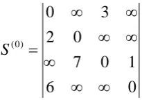
From the figure 4 it clear that the communication path cost is given to the edges of the networking model. Now, convert the above networking model into dependency matrix form
0
6
1
0
7
0
2
3
0
) 0 (
∞
∞
∞
∞
∞
∞
∞
=
S
[image:4.595.382.485.292.364.2]Figure 5: Dependency Matrix of Figure 4
Figure 5 is the dependency matrix of the Figure 4: Networking diagram between 4 numbers of database servers, now applying proposed algorithm to find the lowest cost commutation path.
[ ]
, min[
( 1)[, ], ( 1)[, ] ( 1)[ , ]]
)
( i j S i j S i k S k j
S k = k− k− + k−
0
9
6
1
0
7
5
0
2
3
0
) 1 (
∞
∞
∞
∞
∞
=
S
Figure 6: After applying Floyd’s on Figure 5
0 9 6
1 0 7 9
5 0 2
3 0
) 2 (
∞
∞ ∞ ∞
=
S
Figure 7: After applying Floyd’s on Figure 6
0 9 16 6
1 0 7 9
6 5 0 2
4 3 10 0
) 3
( =
S
Figure 8: After applying Floyd’s on Figure 7
S1
S2
S3
S1
S2 S3
S1
S2
S3
S1
S3
S2
[image:4.595.57.262.308.388.2]Rakesh Kumar Pandey et al, International Journal of Advanced Research in Computer Science, 8 (8), Sept–Oct 2017,163-167
0
9
16
6
1
0
7
7
6
5
0
2
4
3
10
0
) 4
(
=
S
Figure 9: After applying Floyd’s on Figure 8
The Proposed algorithm consist the three loops to find the lowest cost communication path of database servers connected. Hence th
proposed algorithm is
Ο
(
n
3)
, wheren
number of vertex of the graph, database servers is connected. The matrix) 4 (
S
gives the minimum cost for the execution of join operation over the distributed database network.V. CONCLUSIONS
The proposed algorithm is used to find out the minimal cost during the execution of join operations over the network. As we know in the distributed database system tables of the database are stored in the different locations of the network, in their case executing a join a operations is most expensive operations. After applying the proposed algorithm we can easily find out the lowest cost communication path for the network to execute join operation. The
of the algorithm is
Ο
(
n
3)
which is same as the number of the database server on network, which is assumed as database server over the network. The above algorithm is simulated using Java Language.VI. REFERENCES
[1] Nilarun Mukherjee, Synthesis of Non Replicated Dynamic Fragment Allocation Algorithm in Distributed Database System”, Published in Proceeding of international conference on advances in Computer Science , 2010
[2] Sakti Pramanik , David Vineyard, “Optimizing Join Queries in Distributed Databases”, IEEE TRANSACTIONS ON SOFTWARE ENGINEERING, VOL. 14. NO. 9, SEPTEMBER 1988
[3] Ramez Elmasri, Shamkant B. Navathe, “Fundamentals of Database System”, Fifth Edition, Pearson Education, Second Impression, pp 894, 2009.
[4] Manik Sharma, Dr. Gurdev Singh, “Analysis of Joins and Semi-joins in Centralized and Distributed Database Queries”, 2012 International Conference on Computing Sciences
[5] M. Tamer Ozsu, Patrick Valduries, “Principles of Distributed Database System”, Second Edition, Pearson Education, pp 169.
[6] Deepak Shukla, Dr. Deepak Arora, “An Efficient Approach of Block Nested Loop Algorithm based on Rate of Block Transfer”, IJCA, Vol.21, No.3, May 2011.
[7] Narasimhaiah Gorla, Suk-Kyu Song, “Subquery allocation in Distributed Database using GA”, JCS & T, Vol. 10, No.1. [8] P. Apers, A. Hevner, and S. B. Yao, “Optimization algorithms
for distributed queries,” IEEE Trans. Software Engineering, vol. SE-9, no. 1, pp. 57-68, Jan. 1983.
[9] E. Babb, “Implementing a relational database by means of specialized hardware,” ACM Trans. Database Syst., vol. 4, no. I , pp. 1- 29, Mar. 1979.
[10] P. Bernstein and D. Chiu, “Using semijoins to solve relational queries,” J. ACM, vol. 28, no. 1, pp. 25-40, Jan. 1981. [11] P. Bernstein, N. Goodman, E. Wong, C. Reeve, and J.
Rothnie, “Query processing in a system for distributed databases (SDD-I),” ACM Trans. Database Sysr., vol. 6, no. 4, pp. 602-625, Dec. 1981.151 D.
[12] R. Epstein, M. Stonebraker, and E. Wong, “Distributed query processing in-a relational database system,” in Proc. ACM SICMOD, May 1978, pp. 169-180.
[13] S. Pramanik and F. Fotouhi, “An index database machine-An efficient m-way join processor,” The Comput. J . , vol. 29, no. 5, pp. 181
[14] S.Lucas, J. Meseguera ,Normal forms and normal theories in Conditional rewriting , Elsevier Journal of Logical and Algebraic Methods in Programming, 85, 67–97, 2016. [15] Zichen X., Yi-Cheng T., and Xiaorui W., Online Energy
Estimation of Relational Operations in Database Systems, IEEE transactions on computers, vol. 64, no. 11, November 2015
[16] Carlos Busso, Soroosh Mariooryad, Angeliki Metallinou and Shrikanth Narayanan, Iterative Feature Normalization Scheme for Automatic Emotion Detection from Speech, IEEE transactions on affective computing, vol. 4, no. 4, october-december 2013
[17] Moussa Demba,” Algorithm for relational database Normalization up to 3NF” International Journal of Database Management Systems (IJDMS) Vol.5, No.3, June 2013
[18] G. Lamperti, M. Melchiori, M. Zanella, On multisets in database systems, in: Proceedings of WOMP, in: Lecture Notes in Computer Science, vol. 2235, , pp. 147–216,2000 [19] Vimala, S., Khanna Nehemiah, H., Saranya, G. and Kannan,
A.“Applying Game Theory to Restructure PL/SQL Code”, International Journal of Soft Computing, Vol.7, No.6, pp.264-270, 2012.
[20] Ashish Kamra and Elisha Bertino,”Design and Implementation of an Intrusion Response System for Relational Databases”, IEEE transactions on knowledge and data engineering, vol. 23, no. 6, june 2011
[21] Dirk Beyer, Andreas Noack, and Claus Lewerentz,” Efficient Relational Calculation for Software Analysis” IEEE transactions on software engineering, vol. 31, no. 2, Feb 2005