Naive Bayes spam filtering using word position based attributes and length sensitive classification thresholds

S. Werner (ed.),Proceedings of the 15th NODALIDA conference, Joensuu 2005, Ling@JoY 1, 2006, pp. 78–87 ISBN 952-458-771-8, ISSN 1796-1114.http://ling.joensuu.fi/lingjoy/

attributes and length-sensitive classification thresholds

Johan Hovold

Department of Computer Science

Lund University

Box 118, 221 00 Lund, Sweden

[email protected]

Abstract

This paper explores the use of the naive Bayes classifier as the basis for

personalised spam filters. Several

machine learning algorithms, includ-ing variants of naive Bayes, have pre-viously been used for this purpose, but the author’s implementation using word-position-based attribute vectors gave very good results when tested on several publicly available corpora. The effects of various forms of attribute se-lection – removal of frequent and infre-quent words, respectively, and by us-ing mutual information – are investi-gated. It is also shown how n-grams,

with n > 1, may be used to boost

classification performance. Finally, an efficient weighting scheme for cost-sensitive classification is introduced.

1

Introduction

The problem of unsolicited bulk e-mail, or

spam, gets worse with every year. The vast

amount of spam being sent wastes resources on the Internet, wastes time for users, and may expose children to unsuitable contents (e.g. pornography). This development has stressed the need for automatic spam filters.

Early spam filters were instances of

knowl-edge engineering and used hand-crafted rules (e.g. the presence of the string “buy now” indi-cates spam). The process of creating the rule base requires both knowledge and time, and the rules were thus often supplied by the devel-opers of the filter. Having common and, more or less, publicly available rules made it easy for spammers to construct their e-mails to get through the filters.

Recently, a shift has occurred as more focus

has been put on machine learning for the

au-tomatic creation of personalised spam filters. A supervised learning algorithm is presented with e-mails from the user’s mailbox and out-puts a filter. The e-mails have previously been classified manually as spam or non-spam. The resulting spam filter has the advantage of being optimised for the e-mail distribution of the indi-vidual user. Thus it is able to use also the

char-acteristics of non-spam, or legitimate, e-mails

(e.g. presence of the string “machine learning”) during classification.

Perhaps the first attempt of using machine learning algorithms for the generation of spam filters was reported by Sahami et al. (1998).

They trained a naive Bayes classifier and

re-ported promising results. Other algorithms

have been tested but there seems to be no clear

winner (Androutsopoulos et al., 2004). The

naive Bayes approach has been picked up by end-user applications such as the Mozilla e-mail

client1 and the free software project

SpamAs-sassin2, where the latter is using a combination

of both rules and machine learning.

Spam filtering differs from other text cate-gorisation tasks in at least two ways. First, one might expect a greater class heterogeneity – it is not the contents per se that defines spam, but rather the fact that it is unsolicited. Similarly, the class of legitimate messages may also span a number of diverse subjects. Secondly, since misclassifying a legitimate message is gener-ally much worse than misclassifying a spam message, there is a qualitative difference be-tween the classes that needs to be taken into account.

In this paper the results of using a variant of the naive Bayes classifier for spam filtering

1_{http://www.mozilla.org/} 2

are presented. The effects of various forms of attribute selection are explored, as are the ef-fects of considering not only single tokens, but rather sequences of tokens, as attributes. An efficient scheme for cost-sensitive classification is also introduced. All experiments have been conducted on several publicly available cor-pora, thereby making a comparison with pre-viously published results possible.

The rest of this paper is organised as fol-lows: Section 2 presents the naive Bayes clas-sifier; Section 3 discusses the benchmark cor-pora used; in Section 4 the experimental re-sults are presented; Section 5 gives a compari-son with previously reported results, and in the last section some conclusions are drawn.

2

The naive Bayes classifier

In the general context, the instances to be clas-sified are described by attribute vectors ~a =

ha1, a2, . . . , ani. Bayes’ theorem says that the posterior probability of an instance~a being of a certain classcis

P(c|~a) = P(~a|c)P(c)

P(~a) . (1)

The naive Bayes classifier assigns to an in-stance the most probable, or maximum a poste-riori, classification from a finite setCof classes

cM AP ≡ argmax c∈C

P(c|~a).

By noting that the prior probability P(~a) in Equation (1) is independent of c, we may rewrite the last equation as

cM AP = argmax c∈C

P(~a|c)P(c). (2)

The probabilities P(~a|c) = P(a1, a2, . . . , an|c) could be estimated directly from the training data, but are generally infeasible to estimate unless the available data is vast. Thus the naive Bayes assumption – that the individual at-tributes are conditionally independent of each other given the classification – is introduced:

P(a1, a2, . . . , an|c) =

Y

i

P(ai|c).

With this strong assumption, Equation (2) be-comes the naive Bayes classifier:

cN B= argmax c∈C

P(c)Y i

P(ai|c) (3)

(Mitchell, 1997).

In text classification applications, one may choose to define one attribute for each word position in a document. This means that we need to estimate the probability of a certain word wk occurring at position i given the tar-get classification cj: P(ai = wk|cj). Due to training data sparseness, we introduce the ad-ditional assumption that the probability of a specific wordwkoccurring at positioniis iden-tical to the probability of that same word oc-curring at position m, that is,P(ai =wk|cj) = P(am = wk|cj) for all i, j, k, m. Thus we esti-mateP(ai=wk|cj)withP(wk|cj). The probabil-itiesP(wk|cj)may be estimated with maximum likelihood estimates, using Laplace smoothing to avoid zero probabilities:

P(wk|cj) =

Cj(wk) + 1 nj+|V ocabulary|

,

whereCj(wk)is the number of occurrences of the word wk in all documents of class cj, nj is the total number of word positions in docu-ments of classcj, and|V ocabulary|is the num-ber of distinct words in all documents. The class priorsP(cj)are estimated with document ratios. (Mitchell, 1997)

Note that during classification, the indexiin Equation (3) ranges over all word positions con-taining words which are in the vocabulary, thus ignoring so calledout-of-vocabulary words.

The resulting classifier is equivalent to a naive Bayes text classifier based on a multino-mial event model (or unigram language model ). For a more elaborate discussion of the text model used, see Joachims (1997) and McCallum and Nigam (1998).

3

Benchmark corpora

The experiments were conducted on the PU corpora3 _{and the SpamAssassin corpus}4_{. The} four PU corpora, dubbed PU1, PU2, PU3 and PUA, respectively, have been made publicly available by Androutsopoulos et al. (2004) in or-der to promote standard benchmarks. The four corpora contain private mailboxes of four dif-ferent users in encrypted form. The messages

3

The PU corpora are available at http://www.

iit.demokritos.gr/skel/i-config/.

4

The SpamAssassin corpus is available at http:

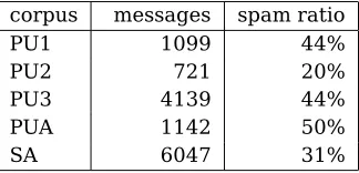
Table 1:Sizes and spam ratios of the five corpora.

corpus messages spam ratio

PU1 1099 44%

PU2 721 20%

PU3 4139 44%

PUA 1142 50%

SA 6047 31%

have been preprocessed and stripped from at-tachments, HTML-tags and mail headers (ex-cept Subject). This may lead to overly pes-simistic results since attachments, HTML-tags and mail headers may add useful information to the classification process. For more infor-mation on the compositions and characteristics of the PU corpora see Androutsopoulos et al. (2004).

The SpamAssassin corpus (SA) consists of private mail, donated by different users, in un-encrypted form with headers and attachments retained5_{. The fact that the e-mails are} col-lected from different distributions may lead to overly optimistic results, for example, if (some of) the spam messages have been sent to a par-ticular address, but none of the legitimate mes-sages have. On the other hand, the fact that the legitimate messages have been donated by dif-ferent users may lead to underestimates since this should imply a greater diversity of the top-ics of legitimate e-mails.

The sizes and compositions of the five cor-pora are shown in Table 1.

4

Experimental results

As mentioned above, misclassifying a legiti-mate mail as spam (L→S) is in general worse than misclassifying a spam message as legiti-mate (S→L). In order to capture such asym-metries when measuring classification perfor-mance, two measures from the field of informa-tion retrieval, called precision and recall, are often used. Denote with|S→L|and |S→S|the number of spam messages classified as legiti-mate and spam, respectively, and similarly for |L→L|and |L→S|. Thenspam recall (R) and

5_{Due to a primitive mbox parser, e-mails}

contain-ing non-textual or encoded parts (i.e. most e-mails with attachments) were ignored in the experiments.

spam precision (P) are defined by

R= |S→S|

|S→S|+|S→L|

and

P = |S→S|

|S→S|+|L→S|.

In the rest of this paper, spam recall and spam precision are referred to simply as recall and precision. Intuitively, recall measures ef-fectiveness whereas precision gives a measure of safety. One is often willing to accept lower recall (more spam messages slipping through) in order to gain precision (fewer misclassified legitimate messages).

Sometimesaccuracy (Acc) – the ratio of cor-rectly classified messages – is used as a com-bined measure.

All experiments were conducted using 10-fold cross validation. That is, the messages have been divided into ten partitions6 _{and at} each iteration nine partitions were used for training and the remaining tenth for testing. The reported figures are the means of the val-ues from the ten iterations.

4.1 Attribute selection

It is common to apply some form of attribute selection process, retaining only a subset of the words – or rather tokens, since punctuation signs and other symbols are often included – found in the training messages. This way the learning and classification process may be sped up and memory requirements are lowered. At-tribute selection may also lead to increased classification performance since, for example, the risk of overfitting the training data is re-duced.

Removing infrequent words and the most fre-quent words, respectively, are two possible ap-proaches (Mitchell, 1997). The rationale be-hind removing infrequent words is that this is likely to have a significant effect on the size of the attribute set and that predictions should not be based on such rare observations anyway. Re-moving the most frequent words is motivated by the fact that common words, such as the En-glish words “the” and “to”, are as likely to occur in spam as in legitimate messages.

6_{The PU corpora come prepartitioned and the SA}

0 20000 40000 60000 80000 100000 120000

0 2 4 6 8 10 12 14

vocabulary size

words occuring less than n times removed PU1 PU2 PU3 PUA SA

Figure 1:Impact on vocabulary size when removing infrequent words (from nine tenths of each corpora).

A very common method is to rank the at-tributes usingmutual information (M I) and to keep only the highest scoring ones. M I(X;C) gives a measure of how well an attribute X discriminates between the various classes inC and is defined as

X

x∈{0,1}

X

c∈C

P(x, c) log P(x, c) P(x)P(c)

(Cover and Thomas, 1991). The probability dis-tributions were estimated as in Section 2. This corresponds to the multinomial variant of mu-tual information used by McCallum and Nigam (1998), but with the difference that the class priors were estimated using document ratios rather than position ratios. (Using word-position ratios gave almost exactly the same classification results.)

In the first experiment, tokens occurring less thann= 1, . . . ,15times were removed. The re-sults indicated unaffected or slightly increased precision at the expense of slightly reduced re-call asngrew. The exception was the PU2 cor-pus where precision dropped significantly. The reason for this may be that PU2 is the small-est corpus and contains many infrequent to-kens. On the other hand, removing infrequent tokens had a dramatic impact on the vocabulary size (see Figure 1). Removing tokens occur-ring less than three times seems to be a good trade-off between memory usage and classifica-tion performance, reducing the vocabulary size with 56–69%. This selection scheme was used throughout the remaining experiments.

Removing the most frequent words turned out to have a major effect on both precision

and recall (see Figure 2). This effect was most significant on the largest and non-preprocessed SA corpus where recall increased from 77% to over 95% by just removing the hundred most common tokens, but classification gained from removing the 100–200 most frequent tokens on all corpora. Removing too many tokens reduced classification performance – again most notably on the smaller PU2 corpus. We believe that this selection scheme increases performance because it makes sure that very frequent tokens do not dominate Equation (3) completely. The greater impact of removing frequent tokens on the SA corpus can thus be explained by the fact that it contains many more very frequent to-kens (originating from mail headers and HTML) (see related discussion in Section 4.2).

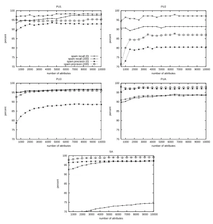
In the last attribute-selection experiment, M I-ranking was used instead of removing the most frequent tokens. Although the gain in terms of reduced memory usage was high – the vocabulary size dropped from 7000–35000 to the number of attributes chosen to be kept (e.g. 500–3000) – classification performance was significantly reduced. When M I-ranking was performed after first removing the 200 most frequent tokens, the performance penalty was not as severe, and usingM I-ranking to se-lect 3000–4000 attributes then seems reason-able (see Figure 3). We are currently investi-gating further the relation between mutual in-formation and frequent tokens.

Since learning and classification time is mostly unaffected – mutual information still has to be calculated for every attribute – we see no reason for usingM I-ranking unless memory us-age is crucial7, and we decided not to use it fur-ther (with unigram attributes).

4.2 n-grams

Up to now each attribute has corresponded to a single word position, or unigram. Is it possi-ble to obtain better results by considering also token sequences of length two and three (i.e. n-grams forn= 2,3)? The question was raised and answered partially in Androutsopoulos et al. (2004). Although many bi- and trigrams were shown to have very high information con-tents, as measured by mutual information, no improvement was found.

7

75 80 85 90 95 100

0 200 400 600 800 1000

percent

n most frequent words removed PU1

spam recall spam precision

75 80 85 90 95 100

0 200 400 600 800 1000

percent

n most frequent words removed PU2

75 80 85 90 95 100

0 200 400 600 800 1000

percent

n most frequent words removed PU3

75 80 85 90 95 100

0 200 400 600 800 1000

percent

n most frequent words removed PUA

75 80 85 90 95 100

0 200 400 600 800 1000

percent

n most frequent words removed SA

Figure 2:Impact on spam precision and recall when removing the most frequent words.

There are many possible ways of extending the attribute set with general n-grams, for in-stance, by using all available n-grams, by just using some of them, or by using some kind of back-off approach. The attribute probabilities P(wi, wi+1, . . . , wi+n|cj) are still estimated us-ing maximum likelihood estimates with Laplace smoothing

Cj(wi, wi+1, . . . , wi+n) + 1 nj+|V ocabulary|

.

Note that extending the attribute set in this way can result in a total probability mass greater than one. Fortunately, this need not be a

prob-lem since we are not estimating the classifica-tion probabilities explicitly (see Equaclassifica-tion (3)).

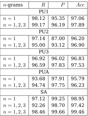
It turned out that adding bi- and trigrams to the attribute set increased classification perfor-mance on all of the PU corpora, but not (ini-tially) on the SA corpus. The various methods for extending the attribute set all gave similar results, and we settled on the simple version which just considers each n-gram occurrence as an independent attribute8. The results are shown in Table 2.

8_{This is clearly not true. The three n-grams in the}

70 75 80 85 90 95 100

1000 2000 3000 4000 5000 6000 7000 8000 9000 10000

percent

number of attributes PU1

spam recall (0) spam recall (200) spam precision (0) spam precision (200)

70 75 80 85 90 95 100

1000 2000 3000 4000 5000 6000 7000 8000 9000 10000

percent

number of attributes PU2

70 75 80 85 90 95 100

1000 2000 3000 4000 5000 6000 7000 8000 9000 10000

percent

number of attributes PU3

70 75 80 85 90 95 100

1000 2000 3000 4000 5000 6000 7000 8000 9000 10000

percent

number of attributes PUA

70 75 80 85 90 95 100

1000 2000 3000 4000 5000 6000 7000 8000 9000 10000

percent

number of attributes SA

Figure 3: Attribute selection using mutual information – spam recall and precision versus the number of retained attributes after first removing no words and the 200 most frequent words, respectively.

The precision gain was highest for the cor-pus with lowest initial precision, namely PU2. For the other PU corpora the precision gain was relatively small or even non-existing. At first the significantly decreased classification per-formance on the SA corpus came as a bit of a surprise. The reason turned out to be that when considering also bi- and trigrams in the non-preprocessed SA corpus, a lot of very fre-quent attributes, originating from mail head-ers and HTML, were added to the attribute set. This had the effect of giving these attributes a too dominant role in Equation (3). By remov-ing more of the most frequent n-grams,

classifi-cation performance was increased also for the SA corpus. The conclusion to be drawn is that mail headers and HTML, although containing useful information, should not be included by brute force. Perhaps some kind of weighting scheme or selective inclusion process would be appropriate.

Table 2: Comparison of classification results when using only unigram attributes and uni-, bi- and tri-gram attributes, respectively. In the experiment n-grams occurring less than three times and the 200 most frequent n-grams were removed. The second n-gram row for the SA corpus shows the result when the 5000 most frequent n-grams were removed.

n-grams R P Acc

PU1

n= 1 98.12 95.35 97.06 n= 1,2,3 99.17 96.19 97.89

PU2

n= 1 97.14 87.00 96.20 n= 1,2,3 95.00 93.12 96.90

PU3

n= 1 96.92 96.02 96.83 n= 1,2,3 96.59 97.83 97.53

PUA

n= 1 93.68 97.91 95.79 n= 1,2,3 94.74 97.75 96.23

SA

n= 1 97.12 99.25 98.95 n= 1,2,3 92.26 98.70 97.42 n= 1,2,3 98.46 99.66 99.46

latter figure may, however, be reduced to 0.7– 4 (while retaining approximately the same per-formance gain) by using mutual information to select a vocabulary of 25000 n-grams.

4.3 Cost-sensitive classification

Generally it is much worse to misclassify legit-imate mails than letting spam slip through the filter. Hence, it is desirable to be able to bias the filter towards classifying messages as legit-imate, yielding higher precision at the expense of recall.

A common way of biasing the filter is to clas-sify a message d as spam if and only if the estimated probabilityP(spam|d)exceeds some thresholdt >0.5, or equivalently, to classify as spam if and only if

P(spam|d) P(legit|d) > λ,

for some real number λ > 1 (Sahami et al., 1998; Androutsopoulos et al., 2000; Androut-sopoulos et al., 2004). This has the same ef-fect as multiplying the prior probability of le-gitimate messages byλand then classifying ac-cording to Equation (3).

As noted in Androutsopoulos et al. (2004), the naive Bayes classifier is quite insensitive to (small) changes to λ since the probability estimates tend to approach 0 and 1, respec-tively. As is shown below, this insensitivity in-creases with the length of the attribute vec-tors, and by exploiting this fact, a more efficient cost-sensitive classification scheme for word-position-based (and hence, variable-length) at-tribute vectors is made possible.

Instead of using the traditional scheme, we propose the following classification criterion:

P(spam|d) P(legit|d) > w

|d|_,

wherew >1, which is equivalent to multiplying each posterior probabilityP(wi|clegit)in Equa-tion (3) with the weight w. Intuitively, we re-quire the spam posterior probability for each word occurrence to be on average w times as high as the corresponding legitimate probabil-ity (given uniform priors).

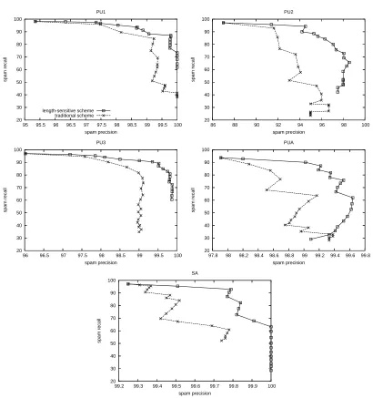
When comparing the two schemes by plot-ting their recall-precision curves for the five benchmark corpora, we found that the length-sensitive scheme was more efficient than the traditional one – rendering higher recall at each given precision level (see Figure 4). This can be explained by the fact that the certainty quotient q(d) = P(spam|d)/P(legit|d)actually grew (de-creased) exponentially with|d|for spam (legiti-mate) messages and thereby made it safe to use much larger thresholds for longer messages. With length-sensitive thresholds we were thus able to compensate for longer misclassified le-gitimate mails without misclassifying as many short spam messages in the process (as would a largeλwith the traditional scheme) (see Fig-ure 5).

5

Evaluation

20 30 40 50 60 70 80 90 100

95 95.5 96 96.5 97 97.5 98 98.5 99 99.5 100

spam recall

spam precision PU1

length-sensitive scheme traditional scheme

20 30 40 50 60 70 80 90 100

86 88 90 92 94 96 98 100

spam recall

spam precision PU2

20 30 40 50 60 70 80 90 100

96 96.5 97 97.5 98 98.5 99 99.5 100

spam recall

spam precision PU3

20 30 40 50 60 70 80 90 100

97.8 98 98.2 98.4 98.6 98.8 99 99.2 99.4 99.6 99.8

spam recall

spam precision PUA

20 30 40 50 60 70 80 90 100

99.2 99.3 99.4 99.5 99.6 99.7 99.8 99.9 100

spam recall

spam precision SA

Figure 4: Recall-precision curves of the two weighting schemes from cost-sensitive classification on the five

corpora using the weightsw= 1.0,1.1, . . . ,2.9andλ= 100,104, . . . ,1076, respectively.

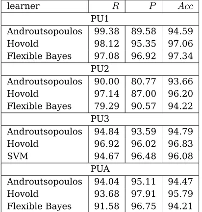
In Androutsopoulos et al. (2004), a variant of naive Bayes was compared with three other learning algorithms: Flexible Bayes, Logit-Boost, and Support Vector Machines. All of the algorithms used real-valued word-frequency at-tributes. The attributes were selected by re-moving words occurring less than four times and then keeping the 600 words with high-est mutual information.9 _{As can be seen in}

9

The authors only report results of their naive Bayes implementation on attribute sets with up to 600 words, but they seem to conclude that using larger attribute sets only have a marginal effect on accuracy.

Table 3, the word-position-based naive Bayes implementation of this paper achieved signifi-cantly higher precision and better or compara-ble recall than the word-frequency-based vari-ant on all four PU corpora. The results were also better or comparable to those of the best-performing algorithm on each corpus.

opti--1500 -1000 -500 0 500 1000 1500

0 200 400 600 800 1000

ln q(d)

document length PU1

spam legit

Figure 5:Certainty quotientq(d) = P_P(₍spam_legit||_dd₎) versus document length (after removing out-of-vocabulary words) for the PU1 corpus. The dashed lines

cor-responds to the constant thresholdsλ = 0(i.e.

un-weighted classification) and λ = 1055_{, respectively,}

and the solid line correspond to the length-sensitive

threshold w|d| _{withw = 2.0. A document dis}

clas-sified as spam if and only ifq(d)is greater than the

threshold in use.

Table 3: Comparison of the results achieved by naive Bayes in Androutsopoulos et al. (2004) and

by the author’s implementation. In the latter,

at-tributes were selected by removing the 200 most fre-quent words as well as words occurring less than three times. Included are also the results of the best-performing algorithm for each corpus as found in An-droutsopoulos et al. (2004).

learner R P Acc

PU1

Androutsopoulos 99.38 89.58 94.59

Hovold 98.12 95.35 97.06

Flexible Bayes 97.08 96.92 97.34 PU2

Androutsopoulos 90.00 80.77 93.66

Hovold 97.14 87.00 96.20

Flexible Bayes 79.29 90.57 94.22 PU3

Androutsopoulos 94.84 93.59 94.79

Hovold 96.92 96.02 96.83

SVM 94.67 96.48 96.08

PUA

Androutsopoulos 94.04 95.11 94.47

Hovold 93.68 97.91 95.79

Flexible Bayes 91.58 96.75 94.21

Table 4: Comparison of the results achieved by naive Bayes on the PU1 corpus in Androutsopoulos et al. (2000) and by the author’s implementation. Re-sults for the latter are shown for both unigram and

n-gram (n = 1,2,3) attributes. In both cases,

at-tributes were selected by removing the 200 most fre-quent n-grams as well as n-grams occurring less than

three times. For each cost scenario, the weightwhas

been selected in steps of0.05in order to get equal or

higher precision.

learner R P

Androutsopoulos (λ= 1) 83.98 95.11 Hovold, 1-gram (w= 1) 98.12 95.35 Hovold, n-gram (w= 1) 99.17 96.19 Androutsopoulos (λ= 9) 78.77 96.65 Hovold, 1-gram (w= 1.20) 97.50 97.34 Hovold, n-gram (w= 1.05) 99.17 97.15 Androutsopoulos (λ= 999) 46.96 98.80 Hovold, 1-gram (w= 1.65) 91.67 98.88 Hovold, n-gram (w= 1.30) 96.04 98.92

mised for each scenario. Table 4 compares the best results achieved on the PU1 corpus10 for each scenario with the results achieved by the naive Bayes implementation of this paper. Due to the difficulty of relating the two differ-ent weights, λ and w, the weight w has been selected in steps of 0.05in order to get equal or higher precision. The authors deemed the λ= 999scenario too difficult to be used in prac-tise because of the low recall figures.

6

Conclusions

In this paper it has been shown that it is pos-sible to achieve very good classification perfor-mance using a word-position-based variant of naive Bayes. The simplicity and low time com-plexity of the algorithm thus makes naive Bayes a good choice for end-user applications.

The importance of attribute selection has been stressed – memory requirements may be lowered and classification performance in-creased. In particular, removing the most fre-quent words was found to have a major impact on classification performance when using word-position-based attributes.

By extending the attribute set with bi- and tri-grams, even better classification performance may be achieved, although at the cost of signif-icantly increased memory requirements.

10

The results are for thebare PU1 corpus, that is,

With the use of a simple weighting scheme based on length-sensitive classification thresh-olds, precision may be boosted further while still retaining a high enough recall level – a fea-ture very important in real-life applications.

Acknowledgements

The author would like to thank Jacek Malec and Pierre Nugues for their encouraging sup-port. Many thanks also to Peter Alriksson, Pon-tus Melke, and Ayna Nejad for useful comments on an earlier draft of this paper.

References

Ion Androutsopoulos, John Koutsias, Konstanti-nos V. ChandriKonstanti-nos, and Constantine D. Spy-ropoulos. 2000. An experimental compar-ison of naive bayesian and keyword-based anti-spam filtering with personal e-mail mes-sages. In P. Ingwersen N.J. Belkin and M.-K. Leong, editors, Proceedings of the 23rd Annual International ACM SIGIR Conference on Research and Development in Information Retrieval, pages 160–167, Athens, Greece.

Ion Androutsopoulos, Georgios Paliouras, and Eirinaios Michelakis. 2004. Learning to fil-ter unsolicited commercial e-mail. Technical Report 2004/2, NCSR "Demokritos". Revised version.

Thomas M. Cover and Joy A. Thomas. 1991. El-ements of Information Theory. Wiley.

Thorsten Joachims. 1997. A probabilistic anal-ysis of the Rocchio algorithm with TFIDF for text categorization. In Douglas H. Fisher, editor, Proceedings of ICML-97, 14th Inter-national Conference on Machine Learning, pages 143–151, Nashville, US.

Andrew McCallum and Kamal Nigam. 1998. A comparison of event models for naive bayes text classification. In Learning for Text Categorization: Papers from the 1998 Workshop, pages 41–48, Madison, Wisconsin. AAAI Technical Report WS-98-05.

Tom M. Mitchell. 1997. Machine Learning. McGraw-Hill.