Parameter Estimation of Exciation Systems

(1)

ABSTRACT

LAI, JUMING. Parameter Estimation of Excitation Systems. (Under the direction of Mesut E. Baran).

The purpose of the research has been to develop a methodology to simplify the

process of parameter estimation of excitation systems. There are two parts in the estimation

process, which are the simulation and the optimization.

For the simulation part, the AC1A excitation system model and AC8B excitation

system model have been implemented in MALTAB/Simulink, based on the IEEE standard

421.5, which is updated in 2005. On the other hand, for the optimization part, the goal is to

look for suitable parameters such that, with the same input, the simulation output will match

the field data from the real machine. We formulated the problem as a least square problem

and applied Damped Gauss-Newton method (DGN) and Levenberg-Marquardt (LM) method

to solve it. We used both the MATLAB Parameter Estimation Toolbox and the MATLAB

programs developed by us to implement the algorithms and get the parameters. For both of

the AC1A models and AC8B, we did the case studies and validation. And this is also a

project sponsored by Progress Energy, who provided two suites of “bump-test” field data of

AC1A excitation system and AC8B excitation system as well. Besides the results, we

determined that the process of parameter estimation of excitation systems would be try DGN

first, and if the simulation response cannot match the measured response well, try LM to get

(2)

Parameter Estimation of Exitation Systems

by Juming Lai

A thesis submitted to the Graduate Faculty of North Carolina State University

in partial fulfillment of the requirements for the Degree of

Master of Science

Electrical and Computer Engineering

Raleigh, North Carolina

2007

APPROVED BY:

Dr. William W Edmonson Jr. Dr. Alex Q Huang

(3)

BIOGRAPHY

Juming Lai was born and grew up in Guangzhou, Guangdong, China on March 5,

1984. Her father is a civil engineer specialized in air transportation that brought her interests

in engineering from her childhood. She showed her interests in math from elementary school,

which helps her a lot in the study of engineering. She entered the South China University of

Technology (SCUT) in Guangzhou in September, 2002 and got her Bachelor degree majored

in Electrical Engineering in June, 2006. And in August of the same year, she entered North

Carolina State University as a master student. She is currently a master student in NCSU and

graduating in December 2007.

She has wide interests, two of which are music and traveling. At the age of 4 years

old, she passed the entrance exam of Xinghai Conservatory of Music in Guangzhou, which

only took 15 students out of 1500, and started learning the piano. Now playing piano

becomes an important hobby of hers. And from she was 5 years old, she with her parents

keeps traveling to either a different province in China or a different country if possible,

which makes her an easy-going person who can communicate well and get well along with

(4)

ACKNOWLEDGMENTS

Firstly, I would like to thank my parents who bring me a family full with love. Thank

my father who can always answer my “whys” and keep me curious to the new things. Thank

my mother who always tries her best to take care of me in every little detail. And then, I

would like to thank my advisor, Dr. Mesut Baran who is professional in academic. He not

only advises me on my research, but also listens to my opinions and tells me how to think

when meeting a new problem. Also, thanks would be truly sent to every instructor who

taught me in the past one and a half year. I did gain a lot from the classes and projects. At last,

I would like to thank all my friends, roommates and colleagues in my lab, SPEC, 1250

Partner I, for all the help for my study and life in NC State.

I would like to acknowledge to Progress Energy, Inc. for sponsoring the research.

And I also acknowledge the Semiconductor Power Electronic Center (SPEC) for providing

(5)

LIST OF TABLES

Table 1 Iteration history of parameter estimation of AC1A starting from typical parameters using DGN ... 40 Table 2 Iteration history of parameter estimation of AC1A starting from typical parameters using LM ... 42 Table 3 Iteration history of parameter estimation of AC1A starting from PL using DGN ... 43 Table 4 Iteration history of parameter estimation of AC1A starting from PL using DGN ... 49 Table 5 Iteration history of parameter estimation of AC1A starting from low parameters using LM ... 51 Table 6 Iteration history of parameter estimation of AC1A starting from PL using DGN ... 53 Table 7 Iteration history of parameter estimation of AC1A starting from high parameters using LM ... 56 Table 8 Iteration history of parameter estimation of AC1A starting from PL using DGN ... 59 Table 9 Iteration history of parameter estimation of AC8B starting from good initial

parametersusing DGN (Unit 1) ... 68 Table 10 Iteration history of parameter estimation of AC8B starting from good initial

(8)

LIST OF FIGURES

Fig. 1. 1 Type AC1A excitation system (Alternator-rectifier excitation system with

non-control rectifiers and feedback from exciter field current) ... 5

Fig. 1. 2 The excitation response from the stage test3... 5

Fig. 2. 1 The real generator and excitation system ... 12

Fig. 2. 2 Inside of the excitation system part ... 12

Fig. 2. 3 The structure of Mark III Brushless exciter... 13

Fig. 2. 4 The circuit of Generator excitation system... 14

Fig. 2. 5 Functional block diagram of a detailed excitation system model [1]... 15

Fig. 2. 6 Simplified functional block ... 15

Fig. 2. 7 A partial AC1A Excitation System Block Diagram Showing Major Functional Blocks ... 16

Fig. 2. 8 A partial AC8B Excitation System Block Diagram Showing Major Functional Blocks ... 17

Fig. 2. 9 Terminal Voltage Transducer and Optional Load Compensation Elements ... 17

Fig. 2. 10 Amplifier model [10]... 18

Fig. 2. 11 Non-windup limiter with sample time constant [1]... 19

Fig. 2. 12 Implementation of non-windup limiter... 19

Fig. 2. 13 Block diagram of an AC exciter ... 20

Fig. 2. 14 AC exciter saturation characteristic... 21

Fig. 2. 15 Rectifier regulation model [10] ... 22

Fig. 3. 1 a simple system for Jacobian approximation test (k=xtest(1), a=xtest(2))... 26

Fig. 3. 2 A sketch map showing how PE toolbox works ... 31

Fig. 3. 3 Optimization environment ... 32

Fig. 4. 1 Test system for estimating parameters of AC1A excitation system... 34

Fig. 4. 2 Implementation of AC1A excitation system in MATLAB/Simulink ... 35

Fig. 4. 3 Model response with typical parameters of AC1A excitation system... 36

Fig. 4. 4 Cost function and step size of each iteration with typical parameters of AC1A excitation system... 37

Fig. 4. 5 Estimated parameters of AC1A excitation system starting from typical parameters37 Fig. 4. 6 Final terminal output of generator with typical parameters of AC1A excitation system ... 38

Fig. 4. 7 Parameter trajectory when estimating parameters of AC1A excitation system ... 39

Fig. 4. 8 Final terminal output of generator starting from typical parameters using DGN .... 41

Fig. 4. 9 Final terminal output of generator starting from typical parameters using LM ... 43

Fig. 4. 10 Final terminal output of generator when estimating AC1A excitation starting from L P using DGN... 45

Fig. 4. 11 Model response with good parameters of AC1A excitation system ... 46

Fig. 4. 12 Cost function and step size of each iteration when estimating AC1A excitation system with good initial paramteres ... 47

(9)

Fig. 4. 14 Final terminal output of generator when estimating AC1A excitation system

starting from good parameters (Grey - Desired curve, Blue – Simulation output)... 49

Fig. 4. 15 Final terminal output of generator when estimating AC1A excitation starting from a good initial point ... 50

Fig. 4. 16 Model response with low parameters of AC1A excitation system ... 51

Fig. 4.17 Final terminal output of generator starting from low parameters using LM ... 53

Fig. 4. 18 Final terminal output of generator when estimating AC1A excitation using DGN starting fromPL... 55

Fig. 4. 19 Model response with high parameters of AC1A excitation system ... 56

Fig. 4.20 Final terminal output of generator starting from high parameters using LM ... 58

Fig. 4. 21 Final terminal output of generator when estimating AC1A excitation using DGN starting from L P ... 60

Fig. 4. 22 Implementation of AC8B excitation system in MATLAB/Simulink... 61

Fig. 4. 23 Model response with good parameters of AC8B excitation system... 62

Fig. 4. 24 Model response with good parameters of AC8B excitation system (Data Unit 2) 63 Fig. 4. 25 Cost function and step size when estimating AC8B excitation system with good initial parameters(Unit 1) ... 64

Fig. 4. 26 Estimated parameters of AC8B excitation system(Unit 1) ... 64

Fig. 4. 27 Final terminal output of generator when estimating AC8B excitation system (Grey - Desired curve, Blue – Simulation output) (Unit 1) ... 65

Fig. 4. 28 Cost function and step size of each iteration when estimating AC8B excitation system (Unit 2)... 66

Fig. 4. 29 Estimated parameters of AC8B excitation system(Unit 2) ... 67

Fig. 4. 30 Final terminal output of generator when estimating AC8B excitation system (Grey - Desired curve, Blue – Simulation output) (Unit 2) ... 68

Fig. 4. 31 Final terminal output of generator when estimating AC8B excitation system (Data Unit 1) ... 69

Fig. 4. 32 Final terminal output of generator when estimating AC8B excitation system (Data Unit 2) ... 70

Fig. 4. 33 Simulation outputs of AC1A excitation system in MATLAB and PSS/E with the parameters provided by Optimization Toolbox ... 72

Fig. 4. 34 Simulation outputs of AC1A excitation system in MATLAB and PSS/E with the parameters provided by Case 1 in section 4.4... 72

Fig. 4. 37 Data plot of responses of bump test from Progress Energy ... 75

Fig. 4. 38 The final plot when estimating the parameters of AC8B excitation system ... 76

(10)

Chapter 1 Introduction

1.1 Background

Today, many of the power system planning and design problems are addressed by

performing system simulations in time domain. The most common studies are small signal,

transient and dynamic stability analyses. Fairly standard models have been developed to

represent the system component for these studies – generators, transmission lines and loads.

One of the main challenges using these simulation tools is the data needed to represent the

system components, as the results are only as accurate as the underlying models and data

used in the computer analysis.

The generators are the most important components in these analyses, and unfortunately,

determining a proper model and the corresponding parameters is the challenge, as it requires

extensive testing of these systems. There are three main components of a generator, which

are the synchronous machine, prime mover (turbine/governor) and the excitation system.

Among these components, the excitation system plays a critical role of providing field

current to the generator, and hence, controlling the terminal voltage of the generator, and also

helping to stabilize the system oscillations after a system disturbance.

To accurately represent the excitation system, it is necessary to have adequate model

structures and suitable parameter values. Models are usually provided by manufacturers or

(11)

representations (Laplace Transform transfer functions). These standards provide suitable

models for different “types” of excitation systems. The standards also provide “typical”

values for each model. Moreover, the manufacturers of the excitation systems provide data

for their excitation systems. Currently it is quite common that in system studies, without any

actual data, the engineers have to choose one of these sources to get the model parameter data

they need for system studies. Another common problem is that the models available on the

commercial software used for the study, such as PSS/E®, may not have the same model

provided by the manufacturer. Hence, the engineer has to translate the data from one model

to another “similar” model.

The need for more accurate equipment models and model parameter identification has

been recognized by organizations responsible for system reliability, such as the North

American Electric Reliability Council (NERC) [4]. NERC requires unit-specific dynamics

data for the dynamic simulations performed by Transmission Planning organizations.

The resulting models provide a much more accurate representation of

generator/excitation system dynamic performance in computer simulations. Some of the

benefits of improved models are as follows.

z Better assessment of a generator’s transient stability margin

z Better assessment of a generator’s dynamic stability margin

z More confidence in simulation results

z Compliance with existing and future NERC reliability data requirements

Model parameters, either manufacturer specified or “typical” values, may be grossly

(12)

individual component separately, without considering the effects of loading conditions, and

the effects of nonlinear interaction between excitation system and the rest of the system [3].

Moreover, parameters change due to retuning, aging, and equipment changes. Therefore,

tools and methods are needed for deriving model parameters from staged tests on the units.

Staged field tests, which provide sufficient information to identifying the parameters, are

divided into two groups [4]. One is collecting steady-state measurements, which includes the

open circuit saturation curve measurement and online measurements. The former one is the

measurement of terminal voltage, field voltage and field current when the generator field

excitation is varied. But for brushless excitation system, only terminal voltage can be

measured. And the later ones are taken at different load level, the typical points of which are

recorded at certain level when the reactive power output changes due to variation of

generator field data. The other step is obtaining the dynamic response. The purpose of the

dynamic tests is to provide a simple and safe disturbance to excite the system. [4] By

comparing the model responses and those obtained from field test, it is obvious to judge the

accuracy of parameters, i.e. the less different the response from each other, the more accurate

the parameter values.

The traditional way to “tune” the parameter is to have skilled engineers select initial

parameters, calculate the difference between measured output and simulation output, and

adjust the parameter to reduce the difference. However, the method requires familiarities

with the equipment functions and the effects of the change of parameters toward the dynamic

response. Unfortunately, such familiarities are quite rare. [4] As a result, the parameter

(13)

1.2 Problem Description

The focus of this thesis is to develop a process or methodology for determining appropriate

parameters of an excitation model selected to represent the specific generator excitation

system under consideration.

For this study, two excitation systems and the models to represent them have been

provided by Progress Energy. Fig. 1. 1 shows one of the models, AC1A, which represents an

Alternating Current (AC) type excitation system. The excitation models are used by the

dynamic simulation package PSS/E, and hence PSS/E will be used to compare and validate

the models to be replicated on Simulink/Matlab. Progress energy has also provided the staged

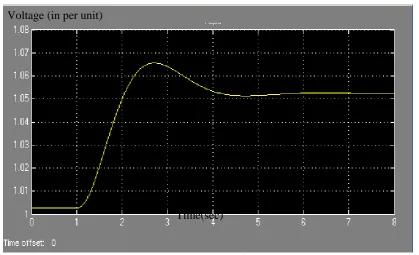
test results for the two excitation systems. Fig. 1. 2 shows the excitation response curve

obtained from the stage tests. As the figure shows, the stage test involves applying a step

change in the set point of the excitation system, which determines the terminal voltage of the

generator, and the response obtained is the output, the terminal voltage of the generator. This

test is referred in practice as the “bump test”. The problem hence is to estimate the

parameters of the selected model such that the response of the model will match the stage test

(14)

Fig. 1. 1 Type AC1A excitation system (Alternator-rectifier excitation system with non-control rectifiers and feedback from exciter field current)

Fig. 1. 2 The excitation response from the stage test

1.3 Related Work

The AC excitation system models represented in IEEE standard 421.5 are nonlinear system

models. Most previous work of parameter estimation of the models was either using linear Time(sec)

(15)

model to approximate the given models, such as the Autoregressive (AR) model, or applying

frequency response techniques to identify the parameters of specific exciters [3 5 6 7].

However, most of these approaches require the output of exciter, which cannot be obtained in

a brushless excitation system. And errors can come from the process of transferring the

parameters in approximated model to the ones of given model. Besides, most of previous

work addressed on their own system models rather than the IEEE standard models.

In [3], a time domain approach has been developed to identify the parameters of AC1A in

IEEE standard 421.5[1]. They used ARX model, a linear discrete time model, to approximate

the transfer function of the system, which is a nonlinear model. ARMAX (Autoregressive

moving average with exogenous input model) model is one of the ARX models. The model

ARMAX(p,q,d) can be represented as

∑

= − = − − = + + + = q i b i i t i i t i i t p i i t

t X d

X 1 1 1 η ε θ ϕ

ε , where

i i i θ η

ϕ , , are parameters, Xt−i is the past value of the signal, εt−i is the error which is

generally assumed to be independent identifically-distributed random variables (i.i.d)

sampled from a normal distribution with zero mean, and d_t−_i is known as the exogenous

input. So a model ARMAX(p, q, d) contains the AR(p) and MA(q) models and a known

external time series d_t. Besides ARMAX model, basic ARX model also includes BJ

(Box-Jenkins) and OE (Output-Error) model, which will be used in different cases.

There are two methods to estimate the coefficients in ARX model structure: Lease square

and Instrumental variables. The author used the least-square method to obtain the parameters

of approximated model. For the optimization algorithm, a Gauss-Newton method was

(16)

the ARX model, the parameter values of AC1A model were estimated.

The advantage of the method is that after getting the linear expression of the system,

many approaches can be used for estimating the parameters of it. They are to increase the

speed of calculation and reduce the cost of it. But the disadvantage is that the approach may

bring more errors when both approximating the system model with the linear one and

transferring the parameters back from the approximated model to the system model.

In [4], a program was developed by using Simulink and Optimization Toolbox in

MATLAB. Simulink allows an easy implementation of the model, in which the system

models are represented in Laplace frequency domain. And the Optimization Toolbox is a

collection of optimization algorithms with graphic user interface. For the least-square curving

fitting problem, the algorithm can be Gauss-Newton and Levenberg Marquardt. Optimization

algorithm determines new parameters and passes it to the Simulink, Simlink then gives the

corresponding response. “A comparison of the simulation output and the desired one is

displayed for each successive pass of the optimization process.” Hence, the users can see

how the response changed to fit the given response during the solution process. The author

gave an example of implementation of IEEE type 1 excitation system.

Simulink is a convenient graphical tool to implement different excitation models. The

user can change a part of the model or the desired curve freely. However, the algorithms are

limited to the ones provided in Optimization Toolbox. Besides, MATLAB is interpretive

language which takes much more time when running the programs in MATLAB, rather than

the compiler languages like C. We tried to use the approach at the beginning of the research,

(17)

Marquardt. In the thesis, we programmed in MATLAB for it have a good communication

with the system model which we have built in MATLAB/Simulink. But for the following

step, we will transplant the program into C or JAVA and have it communicate with the

developed model in PSS/E, which is commercial simulation software.

In [5], a time domain method has been developed to identify IEEE- DC1 and IEEE-

AC1A model parameters. Similar to the approach in [3], the author used a discrete time

model to approximate the system model. Then the least-square method was used to construct

the objective function of the problem. But the difference is that in this paper, they use

stochastic approximation (SA) to find the point at which the objective function can be

minimized to get the parameters. The optimization theory includes two branches known as

deterministic optimization and stochastic optimization. And the stochastic approximation

(SA) is a cornerstone of stochastic optimization. SA methods are used whenever the noise in

the data cannot be ignored. So the SA method creates stochastic equivalents to the classical

conjugate gradient methods. An implementation of SA method is shown in the paper to

estimate the parameters of AC1 type excitation system. In our case, the noises of signals are

in tolerance, so that we did not get into SA methods.

In [6], the discrete-time ARMA (Autoregressive moving average) model was used to

approximate each block of the model by matching the frequency response of them. ARMA

model is also known as Box-Jenkins models, which is one of the ARX models. The model

consists of two parts, autoregressive (AR) part and a moving average (MA) part. [14] The

former part is to represent the signal by itself and the later part is to represent the signal by

(18)

(i.i.d.), sampled from a normal distribution with zero mean (εt ~ N(0,σ2) ). In the paper,

the author obtained parameters of approximated ARMA model of each system block and

then transferred them back the ones of excitation system model. The approach is similar with

the one in reference [3], but the ARMA model would be simpler in this paper, for the author

approximated the block of the excitation system separately. We did not choose it because

both the approximated model may bring more error and we cannot have so much real data

from industry, especially for the brushless machines.

In [7], parameter estimation was performed in frequency-domain. The author utilized

FFT and complex curve fitting technique to estimate the parameters of a excitation system

model, which is a model developed by Taiwan Power Company. About the curve fitting, the

main topics include scatter plot, least square regressions (linear and nonlinear), correlation,

normal probability plots and residual plot. Among them, the nonlinear least square regression

is widely used, which nicely integrates algebra and statistics. A modified weighted least

square (WLS) is described in the paper to obtain the objective function of the curve fitting

problem. Then the author performed Fourier Transformation on the time domain responses

to an injected wide-bandwidth signal of the system to obtain the frequency response data, in

order to estimate the parameters of the model. We did not choose the method for we did not

consider the noise of the signal in the problem.

To sum up, the main considerations of choosing algorithms are the speed of convergence,

the cost of calculations and the accuracy of the results. And for adopting the algorithm, we

have to consider the limitation of tool and data available. Therefore, we plan to develop an

(19)

which, when we got data from stage test, we can get the appropriate parameters of the model

correspondingly.

1.3.1 Scope of the Thesis:

The study involved first getting a general understanding of each component of the model.

Then, models have been implemented in Simulink and verified by using PSS/E. Then a

literature review has been conducted. After the review of related work on this problem, we

adopted the least square approach to estimate the model parameters. Two optimization

methods have been adopted and implemented to solve the least square problem. Two

excitation systems have been used to test and assess the performance of the proposed method.

1.4 Abbreviation

IEEE Institute of Electrical and Electronics Engineering

NERC North American Electric Reliability Council

AC Alternating Current

ARMAX Autoregressive Moving Average with Exogenous input model

BJ Box-Jenkins

OE Output-Error

SA Stochastic Approximation

ARMA Autoregressive Moving Average

GLS Generalized Least Square

(20)

Chapter 2 AC Excitation System Model

2.1 Overview

To capture the behavior of synchronous machine accurately in power system stability studies,

it is essential that their excitation systems are modeled in sufficient detail. The models must

be suitable for representing the actual excitation equipment performance for large, severe

disturbances as well as for small perturbations. [8] Based on excitation power source,

excitation systems are categorized into three groups showing as follows, in which the AC

excitation systems are what we are concerning in the thesis.

Type DC Excitation Systems which utilized a direct current generator with a

commutator as the source of excitation system power. [9]

Type AC Excitation Systems which use an alternator (ac machine) and either

stationary or rotating rectifiers to produce the direct current needed for the generator field.

Type ST Excitation Systems in which excitation power is supplied through

transformers and rectifier.

(21)

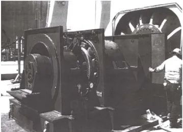
Fig. 2. 1 The real generator and excitation system

Fig. 2. 2 Inside of the excitation system part

(22)

Fig. 2. 3 The structure of Mark III Brushless exciter

Brushless Exciter

Main Generator

(23)

Fig. 2. 4 The circuit of Generator excitation system

In figure 2.5 there is a general functional block diagram, which shows various

synchronous machine excitation subsystems with a common nomenclature performed in

IEEE std 421.5. Showing in the diagram, the terminal output voltage is sent to the excitation

control elements as a feedback signal (V_C and V_S). So when V_T is unstable, the control

elements provide VR to control the output of exciter, i.e. adjust the field voltage and field

current to have VT back to steady state. VREF is an important input of the control part of

excitation systems. Dynamic responses will be recorded, when a step signal is input to the

REF

V port. And comparing dynamic responses of simulation output and the ones from real

machine is the method which is used to ensure the accuracy of models. VOEL and VUEL

describe the output signals from overexcitation limiters and underexcitation limiters,

respectively, the modeling of which have become a very popular topic recently. [1] V_R,

which is the output of voltage regulator, controls the field voltageE_FD, in order to control the

(24)

Fig. 2. 5 Functional block diagram of a detailed excitation system model [1]

To simplify the problem, the “terminal voltage transducer and load compensator” and

“power system stabilizer and supplementary discontinuous excitation controls” are not

considered in the thesis. We can simply represent the block as shown in figure 2.6, in which

the excitation system includes both excitation control elements and exciter.

Fig. 2. 6 Simplified functional block

2.2 Per Unit System

The per-unit system is the expression of system quantities as fractions of a defined base unit

quantity. [10] i.e. the signals in per-unit systems are normalized to some defined bases. Generator

Excitation System VREF

(25)

Firstly, we can define one per unit generator voltage as rated voltage. One per unit exciter

output voltage is that voltage required to produce rated generator voltage on the generator air

gap line.

Also, excitation system models must interface with the synchronous machine model at

both the field terminals and armature terminals. The input control signals to the excitation

system are the synchronous machine stator quantities and rotor speed. The per-unit systems

used for expressing these input variables are the same as those used for modeling the

synchronous machine. Thus, a change of per unit system is required only for those related to

the field circuit.

2.3 AC Excitation System Model Examples

The AC1A excitation model and AC8B excitation model are shown in Figure 2.7 and Figure

2.8, respectively.

AC1A Excitation System

Fig. 2. 7 A partial AC1A Excitation System Block Diagram Showing Major Functional Blocks

Excitation Control Elements

Exciter

(26)

AC8B Excitation System

Fig. 2. 8 A partial AC8B Excitation System Block Diagram Showing Major Functional Blocks

2.4 Model Details for the Excitation Systems

2.4.1 Terminal Voltage Transducer and Load Compensator Models

These are the components that transmit the terminal voltage back to the input of the

excitation systems.

Fig. 2. 9 Terminal Voltage Transducer and Optional Load Compensation Elements

VT: Terminal voltage

T

I : Terminal current

C C jX

R + : Load compensator impedance

R

T : Regular input filter time constant

Exciter

(27)

2.4.2 Amplifier

Amplifier, represented as the main regulator transfer function, may be the magnetic,

electronic or rotating type. The first two types can be represented by the block diagram of

figure 2.10.

Fig. 2. 10 Amplifier model [10]

A

K : Voltage Regular Gain

A

T : Voltage amplifier time constant

max

R

V : Maximum value of VR

min

R

V : Minimum value of VR

Non-windup limiter

(28)

and implementation of which is shown in Figure 2.11 and Figure 2.12, respectively. Then in

principle, we have:

f= Vi−V0 /TA

if V0 ₌VRmax _{, and f > 0, then}dy/dt _{is set to 0}

if V0 ₌VR min_{, and f < 0, then}dy/dt _{is set to 0}

otherwise, VR min_<V0 _<VRmax _{, then}dy/dt _{= f.}

Fig. 2. 11 Non-windup limiter with sample time constant [1]

Fig. 2. 12 Implementation of non-windup limiter

2.4.3 Exciter

The exciter is the part in excitation system which connects to generator. It is the component

who provides the field current to excite the generator. Among the blocks, the vx =VESE(VE)

(29)

always approximated by BEXEX

EX X E X

X E S E A e

V = * ( )= .

Fig. 2. 13 Block diagram of an AC exciter

E

T : Exciter time constant

E

V : Exciter internal voltage

E

S : Saturation function

E

K : Exciter constant related to self-excited field

FD D I

K * : Armature reaction demagnetizing effect.

D

(30)

2.4.3.1 Saturation Function

Saturation function (per unit):

B B A E

SE X

− =

) (

Fig. 2. 14 AC exciter saturation characteristic

2.4.4 Rectifier

Rectifier is to transfer the Alternative current to direct current, which is required for the field

(31)

Fig. 2. 15 Rectifier regulation model [10]

EFD: exciter output voltage(applied to generator field)

EFD = FEX * VE: a function of commutation voltage drop

IFD: generator field current

IN: exciter internal current

FEX = f(IN): the three modes of rectifier circuit operation

Mode 1: f(IN)=1.0−0.577IN, if IN ≤0.433

Mode 2: f(IN)= 0.75−IN2,if0.433<IN <0.75

Mode 3: f(IN)=1.732(1.0−IN),if0.75≤IN ≤1.0

N

I should not be greater than 1.0, but if it is, F_EXshould be set to zero.

2.5 Summary

There are three basic elements of an excitation system: excitation control components,

exciter and rectifier. Besides, terminal voltage transducer and compensator components, and

power system stabilizer are additional ones to keep terminal output voltages stable. To know

the typical structure of each functional block and understand the function of each suite of

blocks in typical models is important in modeling an accurate excitation system and

(32)

Chapter 3 Parameter Estimation using Least Square Method

Since we want the simulation output of excitation model to follow the measured response at

each time point, we can model the problem as a least square problem. To solve this least

square problem, we tried the Damped Gauss Newton method and Levenberg Marquardt

method, which are two basic method for non-linear optimization problems, to get the local

solution of the least square problem.

3.1 Objective function

Let’s restate the problem. It is a nonlinear least squares problem with an objective function

of the form

) ( ) ( 2 1 ) ( 2 1 ) ( 1 2 t R t R x r x f T M i i = =

∑

= (3.1)

in which ri(x)=vi(t:x)−~vi(t),1≤i≤M,t =1,2,..., the vectors viand v~ are the simulation i

output of an nonlinear model and the measured output of the terminal voltage of the

generator, respectively, the vector R=(r₁,r₂,...,r_M)is called the residual,

andx=(p1,p2,...,pN)Tis the vector of unknown parameters. M is the number of

observations and N is the number of parameters. For these problems, M>N, so we say the

problem is an overdetermined problem.

(33)

measure data with model function vi(x), which has nonlinear dependence on variables x.

The best approximation means that the sum of squares of residuals ri(x) is the lowest

possible.

The M×N Jacobian R'of R is defined by

N j M i x r x R j i

ij _∂ ≤ ≤ ≤ ≤

∂

= 1 , 1 ))

( '

( (3.2)

With this notation, it is easy to show that

N T R x R x R x

f = ∈

∇ ( ) '( ) ( ) (3.3)

The necessary conditions for optimality imply that at the minimizerx*,

0 ) ( ) (

' x* R x* =

R T (3.4)

There are two main algorithms for solving least square problems, Gauss-Newton method

and Levenberg-Marquardt method, which will be introduced as follows.

3.2 Gauss Newton method [12]

Steps of Gauss-Newton method

• set xc =x0.

• While ∇f(x_c)>τ_rτ₀ +τ_a & iteration < iteration_max. (τ =(τ_r,τ_a)is the termination

criteria)

(a) Compute the step s

(b) x_t =x_c+s

(34)

The Gauss-Newton(GN) algorithm computes the step s as ) ( ) ( ' )) ( ' ) ( ' ( ) ( )) ( ' ) ( '

( 1 1 c

T c c T c c c T

c R x f x R x R x R x R x

x R

s=− − ∇ =− − (3.5)

where R' is the Jacobian of R.

3.3 Calculating the Jacobian numerically

Since the GN method requires computing the gradient∇f(x), we need to get Jacobian, since

) ( * ) ( ' )

(x_c R x_c R x_c

f =

∇ (3.6)

Since we have the model simulated in MATLAB simulink, rather than a formula expression

of the system, we used the Finite Difference Method to obtain an approximated Jacobian.

There are three forms of the method, which include forward difference method (formula 3.7),

backward difference method (formula 3.8), and central difference method (formula 3.9). The

central difference method is chosen, for in principle it will bring less errors than either of the

other two does.

Forward difference method :

h x f h x f x

f'( ) ( 0 ) ( 0)

0

− +

= (3.7)

Backward difference method :

h h x f x f x

f'( ) ( 0) ( 0 )

0

− −

= (3.8)

Central difference method:

h h x f h x f x f 2 ) ( ) ( ) (

' 0 0

0

− −

+

= (3.9)

Verification of getting Jacobian using central difference method

(35)

identify the two unknown parameters (k and a) of a system a s

k

+ (Figure 3.1) by minimizing

the difference of a numerical prediction and measured data.

Fig. 3. 1 a simple system for Jacobian approximation test (k=xtest(1), a=xtest(2))

Let x=(k,a)T be the vector of unknown parameters. When the dependence on the

parameters needs to be explicit, we will write v(t:x) instead ofv(t). If the outputs are

sampled at M

j j

t } ₁

{ ₌ , wheret_j =(j−1)T/(M−1), then the observation for output will be M j j

v } ₁ { ₌ ,

then the object function is

) ( ) ( 2 1 ) : ( 2 1 ) ( 1 2 x R x R u x t u x f T M j j = − =

∑

= (3.10)

on the interval [0,T], where R(x)=

[

u(1:x)−u1, u(2:x)−u2, L u(M:x)−uM

]

T

The Jacobian of f is

⎥ ⎥ ⎥ ⎥ ⎥ ⎥ ⎥ ⎦ ⎤ ⎢ ⎢ ⎢ ⎢ ⎢ ⎢ ⎢ ⎣ ⎡ ∂ ∂ ∂ ∂ ∂ ∂ ∂ ∂ ∂ ∂ ∂ ∂ = a x M u k x M u a x u k x u a x u k x u x R ) : ( ) : ( ) : 2 ( ) : 2 ( ) : 1 ( ) : 1 ( ) ( ' M M (3.11) Where h h k t u h k t u k x t u 2 ) : ( ) : ( ) : ( ₌ + − − ∂ ∂

,t=1,2,...,M

(36)

Jac_true = 0 0 0.0906 -0.0175 0.1648 -0.0616 0.2256 -0.1219 0.2753 -0.1912 0.3161 -0.2642 0.3494 -0.3374 0.3767 -0.4082 0.3991 -0.4751 0.4174 -0.5372 0.4323 -0.5940 0.4446 -0.6454 0.4546 -0.6916 0.4629 -0.7326 0.4696 -0.7689 0.4751 -0.8009

Absolute error:

Jac_true – Jac_approx =

0 0 -0.0000 -0.0002 -0.0001 -0.0003 -0.0001 -0.0003 -0.0001 -0.0002 -0.0001 -0.0001 -0.0001 0.0001 -0.0001 0.0003 -0.0001 0.0006 -0.0001 0.0009 -0.0001 0.0013 -0.0000 0.0017 -0.0000 0.0022 -0.0000 0.0026 -0.0000 0.0031 -0.0000 0.0035

Relative error: true Jac approx Jac true Jac _ _ _ − =

NaN NaN -0.0004 0.0108 -0.0003 0.0046 -0.0003 0.0024 -0.0003 0.0013 -0.0002 0.0005 -0.0002 -0.0002 -0.0002 -0.0007 -0.0002 -0.0012 -0.0001 -0.0017 -0.0001 -0.0022 -0.0001 -0.0027 -0.0001 -0.0031 -0.0001 -0.0036 -0.0001 -0.0040 -0.0001 -0.0044

) ( ) ( ' ) ) ) : ( ( ) : ( ) ) : ( ( ) : ( ( ) ( 1 1 x R x R u x t u a x t u u x t u k x t u x f j M j j M j = − ∂ ∂ − ∂ ∂ = ∇

∑

= = (3.12)

By using the time domain solution of the system a s

k

+ , we have the function analytically:

f(t) = (1 at) e a

k ₋ −

(3.13)

As a result, the exact Jacobian can be calculated.

Selecte k=4 a=2 as the optimum parameters and use k=5 a=2.5 as the initial points in

simulation. The results are as follows:

Jac_approx= 0 0 0.0907 -0.0173 0.1649 -0.0613 0.2257 -0.1216 0.2754 -0.1910 0.3161 -0.2641 0.3495 -0.3374 0.3768 -0.4085 0.3991 -0.4757 0.4174 -0.5381 0.4324 -0.5953 0.4446 -0.6471 0.4547 -0.6937 0.4629 -0.7352 0.4696 -0.7720 0.4751 -0.8044

As listed above, the errors are very small, so that we can use approximated Jacobian instead

(37)

3.4 Damped Gauss-Newton method

The Gauss-Newton (GN) direction is a descent direction, but the GN method do not have a

good global convergence performance. When the initial iteration is near the solution, it dose

not suffer from poor scaling of f and converges rapidly. However, when far away from the

solution, the Hessian of GN may not be positive definite and the method will fail. To apply

the Newton method to a global convergence problem, the combination of

Gauss-Newton direction with Armijo rule is made, which is called damped Gauss-Gauss-Newton.

Armijo rule

The Armijo rule is based on a general convergence theorem showing that modified steepest

descent algorithms converge under some conditions.

Principal: If λ is an arbitrarily assigned positive number, λm =λ/2m−1,m=1,2,...,and

) (

1 k m k

k x f x

x

k∇

− =

+ λ , where mk is the smallest positive integer for which

,... 2 , 1 , 0 , ) ( ) ( )) (

(x − ∇f x − f x < ∇f x 2 k =

f k λm_k k k αλm_k k (3.14)

Then the sequence {xk}∞k₌0 converges to the point *

x which minimizes f.

Steps of Damped Gauss-Newton method

1 xc =x0.

2 While ∇f(x_c)>τ_rτ₀+τ_a & iteration < iteration_max. (τ =(τ_r,τ_a)is the termination

(38)

(a) Compute the direction of a new step dc.

(b) Set the step size λ=1

(c) x_t =x_c+λd_c.

(d) Compute ∇f(xt)

(i) Apply Armijo rule to find an appropriate λm

(ii) Update x_t and ∇f(x_t)

3.5 Levenberg-Marquardt Method

The damped Gauss Newton algorithm is effective when used for solving zero residual and

small residual problems. But it may fail when the condition number of the matrix

)} ( ' ) ( '

{ T _c

c R x

x

R is too small. Therefore, for the medial residual problems,

Levenberg-Marquardt method is chosen.

The Levenberg-Marquardt methods add a regularization parameter v>0to

)} ( ' ) ( ' { c T c R x

x

R in determining the step s

s=−(v_cI+R'(x_c)TR'(x_c))−1R'(x_c)TR(x_c) (3.15)

where Iis the N×N identity matrix. The matrix v_cI+R'(x_c)TR'(x_c) is positive definite.

And again, if combining the Levenberg-Marquardt with Armijo rule, it become a globally

convergent method for the overdetermined least squares problems.

3.6 Approach I: MATLAB/Simulink Parameter Estimation Toolbox

(39)

Gauss-Newton (GN) and Levenberg-Marquardt (LM) methods to solve the least square

problem. The Gauss-Newton method is given as the “fast” option that provides more precise

results, but it may fail when the initial guess for the parameters are far from the solution. It

quits when the condition number of matrices in the algorithm is too low or the step length is

too small. The condition number is a ratio of the largest singular value to the smallest. The

toolbox offers also the “robust” option which uses the Levenberg-Marquardt when

Gauss-Newton quits [14]

To facilitate modeling of the system, the toolbox has interface with the simulink.

Hence, the model can be developed in simulink. During iterations, the PE toolbox sends the

adjusted parameters to the simulink and gets the simulation results from it. The iterations will

be terminated generally when either the difference between two curves is smaller than the

tolerance that we set before, or the algorithm quits as mentioned before.

3.6.1 Simulink in MATLAB

Simulink is a graphical tool for modeling, simulation and analysis of dynamic systems, in

which the systems can be represented by blocks in frequency domain as the ones shown in

IEEE std 421.5[1]. Most of the blocks with certain functions can be found in Simulink library,

a database in MATLAB, and users can write their own ones by using the “s-function” blocks.

With the initial parameters, when the structure of a system is decided, the simulation can be

implemented by simply drawing the blocks from the library to Simulink window, connecting

(40)

3.6.2 Parameter Estimation (PE) toolbox in MATLAB

Optimization Tool box is a collection of routines that extend the capability of MATLAB for

problems as nonlinear minimization, equation solving and curve fitting. [3] And the PE

toolbox is actually an interface which has the optimization toolbox and the system model in

Simulink communicate to each other. (Figure 3.2) Moreover, both of PE toolbox and

Simulink have a good communication with workspace in MATLAB. For nonlinear least

squares and curve-fitting problems, the desired curve data and initial parameter values can

be saved in workspace and input to the toolbox by selecting the names of the vectors

correspondingly. The algorithms are mentioned in the previous section. And the output

results, which will be shown in the interface of PE toolbox, include the solutions that

minimize the difference of between simulation output and desired curve data, and a record of

cost function and step size of each iteration.

Fig. 3. 2 A sketch map showing how PE toolbox works

3.7 Approach II : Parameter estimation using LM & DGN

Instead of of Simulink and the existed methods in Optimization toolbox in MATLAB, we

would like to use other simulation tools. At this rate, we may be able to simulate the system

faster using software developed for power system simulation such as PSS/E, and implement

more algorithms to efficiently and accurately estimate the parameters.

The interaction between the simulation tool and optimization tool is shown in Figure 3.3. PE Toolbox

Simulink system model

(41)

With initial parameters, simulation output will be obtained from simulation box, which will

be entered into some optimization programs, in which the difference of simulation output and

desired output will be calculated. If the difference does not satisfy the requirement, the

program will adjust the parameter values and get a set of new parameters. With the new

parameters, the system simulates again and produces another suite of outputs.

Fig. 3. 3 Optimization environment

As the first step of the implementation, we will use the simulink for simulation, and

implement the optimization algorithms in Matlab. Later on, after making sure the program do

perform well, we will transplant the program into other computer languages, such as Java or

C and use other simulation tool like PSS/E or ETAP to provide the simulation output.

In this thesis, we tried to program the codes of damped Gauss Newton method, which is a

typical global optimization method for the nonlinear parameter identification. The results of

the implementation of the program on AC1A and AC8B excitation system will be given in

the next chapter.

3.8 Summary

We have got two algorithms and two approaches for solving the least squares problem in

order to estimate the parameter of excitation system. The algorithms used for least square SIMULATION

(Simulink) (PSS/E)

OPTIMIZATION (Optimization Toolbox)

(42)

problems are Gauss-Newton (GN) method and Levenberg-Marquardt (LM) method. GN is

effective when there is a good initial guess, but may quit when the initial guess is bad, while

LM will always gives a result when the initial guess is far from the solution, but not as

effective as GN does. By combining either of the algorithm with Armijo rule, it can be

applied to a global convergence problem, for the Armijo rule is for making sure that the step

sizes sufficiently decrease.

For solving the parameter estimation problem, we developed two approaches. One is to

estimate the parameter of excitation system with MATLAB/Simulink and Parameter

Estimation (PE) Toolbox in MATALB, which already has a collection of functions for

solving the least square problem. The other one is to do parameter estimation with

MATLAB/Simulink and the program developed by ourselves. We are using the same

algorithms with the ones used in PE Toolbox, so that we can compare the results of them.

And then, in the following work, we can transplant the algorithm to C or Java to increase the

speed of operation. Moreover, we may try to implement other algorithms other than the two

(43)

Chapter 4 Case Studies and Validations

Progress Energy gave us the data from “bump test”, we are using the data to test the method

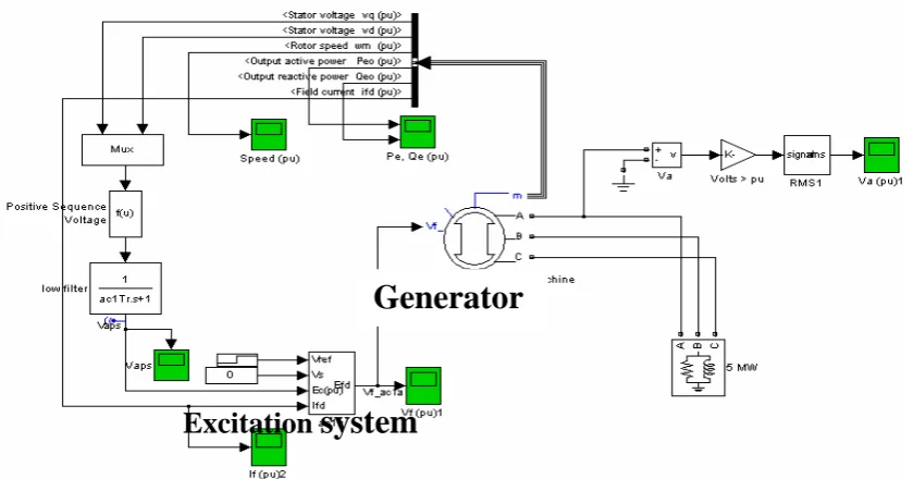
for parameter estimation. As mentioned in Chapter 1, the system consists of a generator and

its excitation system, shown in Figure 4.1. The generator is set to rotate as the speed of 1 p.u.

(per unit). The excitation system gets the terminal voltage as the feedback from generator and

provides the excitation voltage to the generator.

Fig. 4. 1 Test system for estimating parameters of AC1A excitation system

Our project sponsor, Progress Energy, has provided two sets of data for the two excitation

systems they had performed the bumped test recently. Both of these excitation systems are

of AC type and hence, we choose AC1A and AC8B models to represent them, as suggested

by the manufacturer and the Progress Energy.

Generator

(44)

4.1 Case 1: AC1A with typical parameters

Before doing the parameter estimation, the excitation system has been simulated in

MATLAB/Simulink, which is shown in Fig. 4.2.

Fig. 4. 2 Implementation of AC1A excitation system in MATLAB/Simulink

There are 6 parameters of this system: ac1Ka, ac1Ta, ac1Te, ac1Kf, ac1Tf, ac1Kc, ac1Kd

Progress Energy has provided the initial values for them, which are basically the typical

values given for this type of exciter:

Regulator gain: ac1Ka = 766 Regulator time constant: ac1Ta = 0.0200 Exciter time constant: ac1Te = 1.3000 Damping filter gain: ac1Kf = 0.0240 Damping filter time constant: ac1Tf = 1.0000 Rectifier loading factor: ac1Kc = 0.4860 Demagnetizing factor: ac1Kd = 0.3556

Fig. 4.3 compares the simulation response with these initial values with the actual

(45)

Fig. 4. 3 Model response with typical parameters of AC1A excitation system

4.1.1 Parameter Estimation Using Matlab PE Toolbox

Firstly, the Matlab PE Toolbox has been used to estimate the parameters based on the bump

test results given in Fig. 4.3. (Blue line) The robust option has been used for the solution.

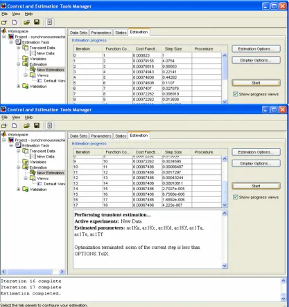
Figure 4.4, shows the iterations that were taken and, cost function and step size of each

iteration. Cost function shows the difference between the simulation output and measured

output. And the step size shows convergence speed. As shown in the figure, the optimization

terminated for the step size is too small, which means the program cannot find a good enough

(46)

Fig. 4. 4 Cost function and step size of each iteration with typical parameters of AC1A excitation system

The Parameters obtained are as follows:

Fig. 4. 5 Estimated parameters of AC1A excitation system starting from typical parameters

(47)

Figure 4.6 compares the simulation response using the estimated parameters with the

measured response.

Fig. 4. 6 Final terminal output of generator with typical parameters of AC1A excitation system (Grey - Desired curve, Blue – Simulation output)

Parameter Trajectory

Sensitivity of parameters is another important issue. With knowing the sensitivity of each

parameter, when manually adjusting the parameters, the engineer can adjust the one who has

the most sensitivity. It will increase the efficiency of the work. From figure 4.5, we can see

(48)

They can be considered as the main factors for the curve fitting, which means that they have

the most sensitivity. There is another plot provided by the PE toolbox, which can also be

used to estimate the sensitivity. That is the parameter trajectory plot (figure 4.7), from which

we can see the changes of parameters by iteration.

(49)

4.1.2 Parameter Estimation using Damped Gauss Newton

As the second option, the damped Gauss Newton Method which has been implemented

in MATLAB codes has been used to estimate the parameters, using the same initial

parameter values. In table 1 listed the iteration history of the operation.

Table 1 Iteration history of parameter estimation of AC1A starting from typical parameters using DGN

Norm(gc) f(xc) Armijo iter. Iteration

0.0034 0.0023 0 0

0.0033 0.0018 9 1

0.0086 0.0018 0 2

0.0036 0.0006 0 3

0.0016 0.0003 0 4

0.0005 0.0002 0 5

0.0002 0.0001 0 6

0.0004 0.0001 0 7

0.0003 0.0001 0 8

0.0004 0.0001 0 9

0.0004 0.0001 0 10

This method yielded the following values:

Xmodel_GN=

ac1Ka ac1Kf ac1Te ac1Tf ac1Ta ac1Kc ac1Kd 669.3898 0.0502 3.0419 1.7159 0.0339 0.5123 -0.3254

Fig. 4.8 compares the simulation response with the test data. As it indicates, it is a good

fit. The method did converge, but did not converge to the best solution. Since we did not

(50)

Fig. 4. 8 Final terminal output of generator starting from typical parameters using DGN

4.1.3 Parameter Estimation using LM and DGN

For improving the result, we choose the combination of Levenberg Marquardt method and

Damped Gauss Newton method. The LM method has been used to get the better start point

L

P first and then DGN method has been used to get the solution. The initial parameters are

the same as the previous case, which is

X0 =

ac1Ka ac1Kf ac1Te ac1Tf ac1Ta ac1Kc ac1Kd 766 0.0200 1.3000 0.0240 1.0000 0.4860 0.3556

4.1.3.1 Levernberg Marquardt

(51)

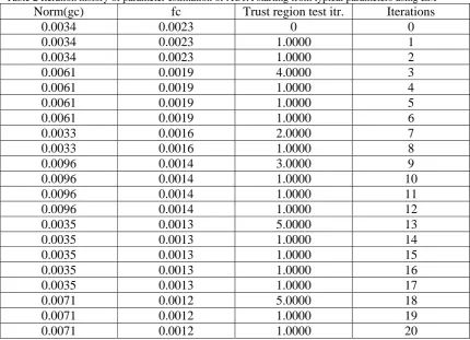
Table 2 Iteration history of parameter estimation of AC1A starting from typical parameters using LM

Norm(gc) fc Trust region test itr. Iterations

0.0034 0.0023 0 0

0.0034 0.0023 1.0000 1

0.0034 0.0023 1.0000 2

0.0061 0.0019 4.0000 3

0.0061 0.0019 1.0000 4

0.0061 0.0019 1.0000 5

0.0061 0.0019 1.0000 6

0.0033 0.0016 2.0000 7

0.0033 0.0016 1.0000 8

0.0096 0.0014 3.0000 9

0.0096 0.0014 1.0000 10 0.0096 0.0014 1.0000 11 0.0096 0.0014 1.0000 12 0.0035 0.0013 5.0000 13 0.0035 0.0013 1.0000 14 0.0035 0.0013 1.0000 15 0.0035 0.0013 1.0000 16 0.0035 0.0013 1.0000 17 0.0071 0.0012 5.0000 18 0.0071 0.0012 1.0000 19 0.0071 0.0012 1.0000 20

Xmodel_LM =

ac1Ka ac1Kf ac1Te ac1Tf ac1Ta ac1Kc ac1Kd 500.8150 0.0271 2.0854 1.0073 0.0186 0.4747 0.3537

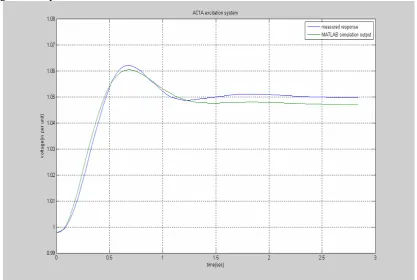
According to the values of cost functions, the iterations converged. It terminated due to

the maximum iteration limit, which means that the program stopped before finding the best

solution. As indicated in the Fig. 4.9, the curves did not match to each other well, for the

(52)

Fig. 4.9 compares the result with data.

Fig. 4. 9 Final terminal output of generator starting from typical parameters using LM

4.1.3.2 Damped Gauss Newton

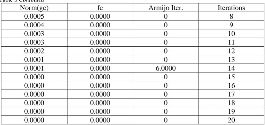
In Table 3 shows the history of the iteration when using Gauss Newton starting from the

parameters getting from Levenberg Marquardt method PL, which is

xstart =

ac1Ka ac1Kf ac1Te ac1Tf ac1Ta ac1Kc ac1Kd 500.8150 0.0271 2.0854 1.0073 0.0186 0.4747 0.3537

Table 3 Iteration history of parameter estimation of AC1A starting from PL using DGN

Norm(gc) fc Armijo Iter. Iterations

0.0006 0.0004 0 0

0.0008 0.0002 0 1

0.0011 0.0001 0 2

0.0011 0.0001 0 3

0.0010 0.0001 0 4

0.0008 0.0001 0 5

0.0007 0.0000 0 6

(53)

Table 3 Continued

Norm(gc) fc Armijo Iter. Iterations

0.0005 0.0000 0 8

0.0004 0.0000 0 9

0.0003 0.0000 0 10

0.0003 0.0000 0 11

0.0002 0.0000 0 12

0.0001 0.0000 0 13

0.0001 0.0000 6.0000 14

0.0000 0.0000 0 15

0.0000 0.0000 0 16

0.0000 0.0000 0 17

0.0000 0.0000 0 18

0.0000 0.0000 0 19

0.0000 0.0000 0 20

xcurrent =

ac1Ka ac1Kf ac1Te ac1Tf ac1Ta ac1Kc ac1Kd

1.0e+003 *

1.0427 0.0001 0.0050 0.0018 0.0001 0.0003 -0.0002

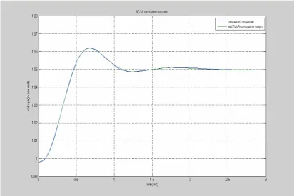
The method did converge. Fig. 4.10 shows that the model response matches the

(54)

Fig. 4. 10 Final terminal output of generator when estimating AC1A excitation starting from PL using DGN

4.2 Case 2: AC1A with good initial paramters

When started with typical parameter values, the two methods did not reach the same solution.

To find a better solution, John O’connor who is the expert on using these models in Progress

Energy, adjusted the parameter values manually to find a better initial point. This new initial

parameters have been given as:

(55)

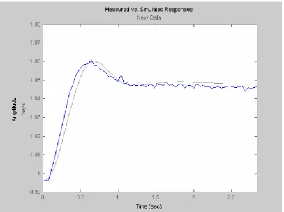
As Fig.4.11 shows these values indeed yield a simulation response that is much closer to the

actual response than that of the original parameter values.

Fig. 4. 11 Model response with good parameters of AC1A excitation system (Grey - Desired curve, Blue – Simulation output)

4.2.1 Parameter Estimation Using Matlab PE Toolbox

For the case, again we tried Matlab PE Toolbox first to estimate the parameters. The fast

option has been used for the solution, for it has good initial points. Figure 4.12 shows the

iterations that were taken and, cost function and step size of each iteration. The program may

not find a good enough solution before it converge, for the optimization terminated for the

(56)

(57)

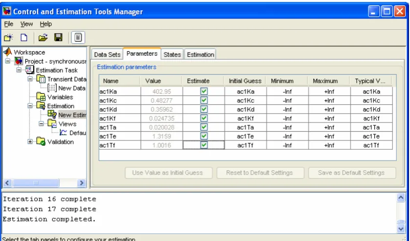
Parameters obtained are:

Fig. 4. 13 Estimated parameters of AC1A excitation system starting from good initial parameters

We get: Initial value: Regulator gain: ac1Ka = 402.95 ac1Ka = 400 Regulator time constant: ac1Ta = 0.020028 ac1Ta = 0.0200 Exciter time constant: ac1Te = 1.3159 ac1Te = 1.3000 Damping filter gain: ac1Kf = 0.024735 ac1Kf = 0.0240 Damping filter time constant: ac1Tf = 1.0016 ac1Tf = 1.0000 Rectifier loading factor: ac1Kc = 0.54693 ac1Kc = 0.4860 Demagnetizing factor: ac1Kd = 0.35962 ac1Kd = 0.3556

Figure 4.14 compares the model response using the estimated parameters with the

(58)

Fig. 4. 14 Final terminal output of generator when estimating AC1A excitation system starting from good parameters (Grey - Desired curve, Blue – Simulation output)

4.2.2 Damped Gauss Newton

The damped Gauss Newton Method implemented in Matlab has also been used to estimate

the parameters using the same initial parameter values. Here we also only use DGN method,

rather than use the combination of GN method and LM method. In Table 4 listed the iteration

history of the operation.

Table 4 Iteration history of parameter estimation of AC1A starting from PL using DGN

Norm(gc) f(xc) Armijo iter. Iteration

0.0237 0.0066 0 0

0.0035 0.0001 0 1

0.0025 0.0001 0 2

0.0012 0.0000 0 3

0.0005 0.0000 0 4

0.0007 0.0000 0 5

(59)

Xmodel=

ac1Ka ac1Kf ac1Te ac1Tf ac1Ta ac1Kc ac1Kd

364.1523 0.0413 1.6724 1.4580 0.0542 0.4860 0.4039

cost: fc = 1.0498e-005

The method converged fast(only 6 iterations) and sufficiently reduced the residuals to 1e-5,

which can tell us DGN method works well. When starting from a good initial points, using

DGN, the iteration converges well and provides good results The terminal output curve is

shown in Fig. 4.15.

Fig. 4. 15 Final terminal output of generator when estimating AC1A excitation starting from a good initial point

4.3 Case 3: AC1A with Low Parameters

To test the method, we tried two more cases using the combination of LM and DGN. One of

(60)

X0 = ac1Ka ac1Kf ac1Te ac1Tf ac1Ta ac1Kc ac1Kd

383.0000 0.0100 0.6500 0.0120 0.5000 0.2430 0.1778

Fig 4.16 shows the simulation with the initial parameters.

Fig. 4. 16 Model response with low parameters of AC1A excitation system

4.3.1 Levernberg Marquardt

Table 5 shows the history of the iteration when using Levenberg Marquardt.

Table 5 Iteration history of parameter estimation of AC1A starting from low parameters using LM

Norm(gc) fc Trust region test itr. Iterations

0.0378 0.0244 0 0

0.0378 0.0244 1.0000 1

0.0378 0.0244 1.0000 2

0.0378 0.0244 1.0000 3

0.0286 0.0096 2.0000 4

0.0286 0.0096 1.0000 5

0.0286 0.0096 1.0000 6

0.0102 0.0046 2.0000 7

Parameter Estimation of Exciation Systems

ABSTRACT

Parameter Estimation of Exitation Systems

BIOGRAPHY

ACKNOWLEDGMENTS

TABLE OF CONTENTS

LIST OF TABLES

LIST OF FIGURES

Chapter 1

Introduction

1.1 Background

1.2 Problem Description

1.3 Related Work

∑

∑

∑

1.4 Abbreviation

Chapter 2

AC Excitation System Model

2.1 Overview

2.2 Per Unit System

2.3 AC Excitation System Model Examples

Excitation Control Elements

Exciter

2.4 Model Details for the Excitation Systems

Exciter

2.5 Summary

Chapter 3

Parameter Estimation using Least Square Method

3.1 Objective function

∑

3.2 Gauss Newton method [12]

3.3 Calculating the Jacobian numerically

∑

[

]

∑

∑

3.4 Damped Gauss-Newton method

3.5 Levenberg-Marquardt Method

3.6 Approach I: MATLAB/Simulink Parameter Estimation Toolbox

3.7 Approach II : Parameter estimation using LM & DGN

3.8 Summary

Chapter 4

Case Studies and Validations

Generator

4.1 Case 1: AC1A with typical parameters

4.2 Case 2: AC1A with good initial paramters

4.3 Case 3: AC1A with Low Parameters