Molecular Characterization of Local Adaptation of Natural Flowering Dogwood Populations (C. florida) to Fungal Pathogens and Environmental Stress

ABSTRACT

PAIS, ANDREW LABEL. Molecular Characterization of Local Adaptation of Natural Flowering Dogwood Populations (C. florida) to Fungal Pathogens and Environmental Stress. (Under the direction of Dr. Qiu-Yun (Jenny) Xiang).

Molecular Characterization of Local Adaptation of Natural Flowering Dogwood Populations (C. florida) to Fungal Pathogens and Environmental Stress

by

Andrew Label Pais

A dissertation submitted to the Graduate Faculty of North Carolina State University

in partial fulfillment of the requirements for the degree of

Doctor of Philosophy

Plant Biology

Raleigh, North Carolina 2017

APPROVED BY:

_______________________________ _______________________________ Dr. Qiu-Yun (Jenny) Xiang Dr. William A. Hoffmann

Committee Chair

_______________________________ _______________________________

Dr. Xu (Sirius) Li Dr. Jean B. Ristaino

DEDICATION

iii BIOGRAPHY

Andrew Pais was born in Atlanta, GA, raised in Knoxville, TN, and has since lived in several towns along I-40. One notable stop was Nashville, TN, where Andrew received a Bachelor’s degree at Vanderbilt University in 2009 and became an enviable talent of the underground country music scene. However, music was not enough to satisfy Andrew’s wonder of the world so he dedicated the remainder of his attention to science—first teaching biology in Greensboro, NC and then specializing in Plant Biology as part of Dr. Jenny Xiang’s lab at North Carolina State University.

According to Andrew’s parents, Andrew acquired an inquisitive mindset very early in life that concerned the true order of the world—often frustrating them with probing questions such as “Can God create a boulder that he cannot lift?” Andrew’s obnoxious questions gradually evolved into an acquired liberal smugness as an undergraduate studying

ACKNOWLEDGMENTS

I’d like to thank my wife Brittany, my constant when everything was variable. Brittany, thank you for loving me at my worst and always encouraging me to go beyond my best.

My gratitude extends to my advisor, Dr. Jenny Xiang, for providing me outstanding opportunities to grow as a researcher and also allowing me to independently develop the foci of my dissertation. I am extremely grateful to have her as a source of unwavering support, and she has always gone out of her way to ensure my success. She has been patient and thorough in helping me revise my chapters, and she has connected me with a series of professional contacts and mentors, whom also deserve my thanks regarding the development of my dissertation project. Dr. William Hoffmann provided valuable advice for collecting and analyzing physiological trait data. Dr. Jean Ristaino provided thorough feedback about the metagenomics analyses conducted. Dr. Sirius Li provided the resources and counsel to implement untargeted metabolomics profiling and various phytochemical analyses. Dr. Ross Whetten provided many resources for preparing and sequencing libraries, and he also trained me in bioinformatics.

v The following people also deserve my appreciation for sharing resources and expertise as part of collaborative projects: William Kohlway, Zhe-Chen (Andres) Qi, Jason Lattier, and Kim Shearer Lattier.

I thank Dr. Margo Daub, Dr. Richard Blanton, the Department of Plant and Microbial Biology, and NC State for providing me opportunities such as the Teaching Assistantship to further my training as a scholar and teacher. Dr. Phillip Wadl and Dr. Jim Leebens-Mack, representing the University of Tennessee (now in USDA ARS) and the University of Georgia respectively, are owed a great deal of gratitude for providing resources and counsel as part of the Dogwood Genome Project, a broader collaborative team warranting my gratitude. The Genome Science Lab at NC State has also been very helpful in sequencing many of our genomic libraries. NC Forest Service, the Nature Conservancy, and land stewards from many national and state parks are owed a great deal of gratitude for the services they provide to researchers such as myself.

In addition, I dedicate immense gratitude to former and current staff from the

Department of Plant and Microbial Biology. Special thanks to Sue Vitello for helping me sort through the University’s administrative paper work. Rachel Clark and Donna Wright were indispensable for helping me collect suitable plant specimens for my teaching

responsibilities, and both helped to train and prepare me for setting up and teaching labs independently. Moreover, I very much enjoyed working with them.

TABLE OF CONTENTS

LIST OF TABLES………...……… ix

LIST OF FIGURES………...……. xii

Chapter 1: Ecological genomics of local adaptation in Cornus florida L. by genotyping by sequencing………. 1

Abstract……….… 2

Introduction………... 2

Materials and Methods……….……... 4

Results………... 8

Discussion………... 11

Conclusions and Future Directions………. 23

Acknowledgements………. 24

References………... 24

Supporting information………... 26

Chapter 2: Discovering variation of secondary metabolite diversity and its relationship with disease resistance in Cornus florida L.………...…… 27

Abstract………... 28

Introduction………. 29

Materials and Methods……….……….….. 32

Results………. 43

vii

References………... 58

Tables………..… 68

Figures……….……… 71

Chapter 3: Congruent patterns of disease and genetic variation along the range of Cornus florida L. ……….………... 79

Abstract………80

Introduction………. 81

Materials and Methods……….…….….. 85

Results………. 96

Discussion……….………… 106

Acknowledgements………..…………. 114

References………..…………... 115

Tables………..……..… 121

Figures………...………… 129

Chapter 4: Fungal community composition of Cornus florida L. revealed by genotype by sequencing and metagenomics………...………... 138

Abstract………..…………139

Introduction………..………. 140

Materials and Methods………...…….….. 142

Results………..………. 149

Discussion……….………… 153

References………..……... 159

Tables………..……..… 164

Figures………...…… 166

Appendices………...……. 173

Appendix A: Chapter 2 supplementary data………...…… 174

ix LIST OF TABLES

Table 2.1 Chart of all predictors considered in current study accompanied with abbreviations used in main text..……….……...68 Table 2.2 Mantel tests of correlations between subpopulation-level metabolic, genetic, and environmental distances. Chemical distance matrix obtained through Analysis of Similarities (ANOSIM) using 377 metabolites. Genetic distance matrix consists of linearized Fst values calculated from 1,171 reference (putatively neutral) SNPs. Site-level means of temperature at collection (Tcol) and precipitation of driest month (Bio14) used for matrices of Euclidean distances, and geographic distance among sites calculated from a X, Y coordinate system. Vertical bar denotes partial Mantel test controlling for third matrix right of “|”..…………...69 Table 2.3 Mixed logistic regression of individual metabolite effects (integrated intensity of chromatogram peak) on log odds of being healthy vs. diseased. Model controls for

inbreeding coefficient (F), temperature at collection (Tcol), and random effect of sites. Reporting six significant features of the 377 chemical features after retaining highest

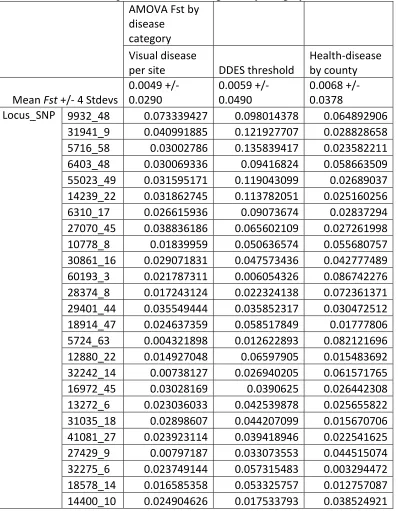
Table 3.3 SNP-specific Fst estimates showing degree of genetic differentiation between a group with no evidence of disease occurrence and a group with evidence of disease

occurrence, depending on the classification system for defining groups. For comparison to each SNP, the mean Fst value of the distribution (plus or minus four standard deviates) is listed in second row. Top 25 (based on average Fst by category) results shown.…...…....125 Table 3.4 Description of Fst outlier loci deviating from a hierarchical null model distribution of expected heterozygosity and Fst. Three hierarchical clusters were defined based on genetic structure results, and eight populations with a sampling of ten or more trees were nested within each cluster (Cluster one: KS-GAL, MO-PC, MO-LO, and MO-CC; Cluster two: MI-BD and MI-FC; Cluster three: NC-RW and SC-PE). Fst outlier analysis was done with the program Arlequin, specifying 20,000 simulations, 100 demes, and 10 groups. After

xi Table 3.6 BLAST hits and annotations for select GBS loci and genome scaffolds of interest featured in discussion.………...………...……..128 Table 4.1 Summary of location, sampling, and conditions of each collection site sampled for Cornus florida leaf tissue. ………...………..…164 Table 4.2 Summary of multivariate linear regression with the proportion of total GBS

LIST OF FIGURES

Figure 2.1 Subset of collections from broader study of C. florida (top) applied to metabolic study of chemical diversity in North Carolinian populations (bottom). Red counties have known incidence of dogwood anthracnose disease. For subset of populations sampled in this study, differences in mean monthly rainfall, length of growing period, soil type, and county occurrence of dogwood anthracnose are visualized to demonstrate the heterogeneity in environment that exists among the mountain, Piedmont, and Coastal Plain ecoregions of North Carolina.………....71 Figure 2.2 Comparison of subpopulation means of (A) observed and (B) expected

heterozygosity, (C) nucleotide diversity, (D) rarefied-allelic richness, (E) inbreeding

xiii Figure 2.3 (A) Medians of individual-level chemical richness values (calculated from 377 metabolites) by health score categories (coded 1-5 with 5 being healthiest). (B) Also depicted are calculations of chemical richness from 377 metabolites, including fragments and adducts (2,785 chemical features). Boxplots depict minimum and maximum values (whiskers), outliers (dots), first quartile, median, and third quartile. The notches in each box correspond to the 95% confidence interval of each median value, and the width of each box is

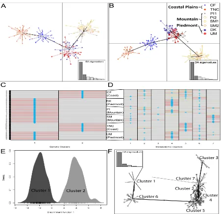
proportional to the square root of each groups’ sample size...73 Figure 2.4 Plots of discriminant analyses of principal components (DAPC) derived from (A) 1,171 reference SNPs or (B) 377 chemical features (highest intensity metabolite per peak group). Dots of different colors and shapes represent individual trees belonging to different collection sites as indicated by legend. Mountain sites are: Smoky Mountains (SM1 and SM2) and Pisgah Forest (PI1 and PI2). Piedmont sites are in Duke Forest (DK) and Umstead State Park (UM), and Coastal Plain sites are in the Croatan forest (CF) and the Nature

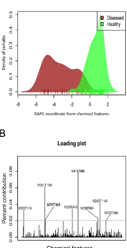
xv Figure 2.7 Density plot of samples representing discriminant analysis of principal

components (DAPC) results with groups defined as samples that are healthy (green) or diseased (red). (B) Loading plot showing metabolites contributing most for distinguishing healthy vs. diseased plants.………..77 Figure 2.8 Top results of biomarkers indicative of healthy or diseased plants from three distinct analytical methods: (A) Partial least squares discriminant analysis (PLS-DA), (B) support vector machines (SVM), and (C) random forests (RF). Metabolites past solid black line on each plot were considered for biomarker selection. Panel right of each support index panel for biomarker tests indicates relative expression of each compound in healthy vs. diseased plants with black shades representing higher expression and white shades

representing lower expression.……….……….…...78 Figure 3.1 Map flowering dogwood range with location of sampling sites indicated in

Figure 3.2 Multiple correspondence (MCA) results and summary of sites with evidence of dogwood anthracnose. (A) MCA was done on categorical data of dogwood anthracnose occurrence (i.e. contaminant sequence thresholds, visual observation of disease per site, and county reports) to obtain reduced-dimension scores spanning low (negative) and high

xvii Figure 3.4 STRUCTURE and discriminant analyses of principal components (DAPC) plots (left and middle columns) with spatial context of the latter genetic structure results (right column). Each row corresponds to four best genetic cluster models (K=2, K=3, K=4, and K=5). STRUCTURE plots show cluster assignment probabilities per individual. Using the same color for each corresponding cluster, middle panel depicts the genetic distance relationships between estimated clusters. According to mean DAPC probabilities of membership per site (as seen on right panels), much of yellow cluster overlaps with populations near or west of the Mississippi Valley (Fig. 3.1) while the blue cluster

Figure 3.6 Comparisons of genetic diversity between samples in areas with no (blue) or some evidence of disease occurrence (red), as defined by different disease occurrence categories (i.e. contaminant sequence thresholds, visual observation of disease per site, and county reports). Genetic diversity characterized by estimates of (A) observed heterozygosity, (B) expected heterozygosity, and (C) nucleotide diversity. Genetic diversity of all samples (grey) also represented for each comparison. While trends indicate that samples in areas with no evidence of dogwood anthracnose disease often have higher genetic diversity, overlapping 95% confidence intervals indicate no significant differences among groups.………...134 Figure 3.7 Discriminant analyses of principal components (DAPC) based on definition of healthy (blue) and diseased (red) groups. Definitions of health-disease categories include a sample (A) occurring in a site with visual absence-presence of disease, (B) occurring in a site that has record of contaminant sequences below-above the designated threshold of 0.1%, or (C) a sample existing in a county with absence or verified occurrence of dogwood

xix Figure 3.8 Gradient forest plots of allelic turnover patterns along (A) latitude, (B) longitude, and (C and D) an incidence gradient of disease estimated from multiple correspondence analysis of three categorical variables of disease occurrence evidence. The cumulative

importance (response variable) is graphed for each line function representing an allele and its turnover pattern along a given gradient. Allele functions are calculated using minor allele frequencies of collection sites from genetic diversity analyses (A, B, and C) or (D) are calculated by presence-absence of the minor allele for all 289 samples. Interesting candidate SNPs—highly predictive for assigning samples into areas of disease absence-occurrence or significantly associated to the MCA disease gradient or other abiotic covariates (LFMM and EMMAX results)—were highlighted different colors in parts A, B, C, and D if they had notable patterns of allelic transition. In panel E, the cumulative importance pattern of all 72 candidate SNPs (orange) is contrasted to patterns of cumulative importance inferred from all 1,078 SNPs (black). Transition zones of particular candidate SNPs are visualized in a spatial context (panel F) corresponding to the colors of highlighted candidate SNPs in panels

A-D……….………...136 Figure 3.9 Illustration of candidate GBS loci alignment to C. florida genome scaffold

Figure 4.1 (A) Map of sampling locations across Flowering Dogwood (Cornus florida) range (gray), including: Ozark/Ouachita gallery forests (Missouri; maroon), Mixed Wood Plains (Michigan and Ohio; yellow), Appalachian mountains (North Carolina; red), Piedmont subpopulations (North Carolina and South Carolina; green), and eastern Coastal Plains (North Carolina, South Carolina, and Florida; orange). Counties highlighted in red have verified reports of dogwood anthracnose, according to US Forest Services whereas sites with visual observation of anthracnose disease (e.g. leaf blotting and necrosis) are indicated with triangular arrows. Climatic relationships of sampling sites depicted as (B) PCA of

xxi Figure 4.3 Notched boxplot representing differences in the proportion of GBS sequences uniquely aligned to either (A) the genome of Erysiphe pulchra (powdery mildew) or (B) Discula destructiva (dogwood anthracnose). Boxplots depict minimum and maximum values (whiskers), outliers (dots), first quartile, median, and third quartile. The notches in each box correspond to the 95% confidence interval of each median value, and the width of each box corresponds to the square root of the sample size for each collection site.………...…168 Figure 4.4 Comparison of fungal species-level operation taxonomic units (OTUs) between (A) 64-128bp GBS sequence matches to UNITE ITS database, (B) 64-128bp GBS sequence matches to Warcup ITS database, and (C) Megablast results from Real-time PCR of ITS region from Miller et al. 2016. Taxonomic ranks from this study (A and B) underlined in crimson if presence of fungi taxa confirmed in literature.……...…169 Figure 4.5 Genus-level fungal operational taxonomic units (OTUs) and their relative

Figure 4.6 Bar graphs depicting fungal community composition differences between Cornus florida sampling sites with any visual evidence of anthracnose disease in early spring and summer (i.e. leaf blotting, necrosis, or branch dieback) and sites with no visual evidence of anthracnose disease. (A) we particularly note proportional differences in class-level operation taxonomic units (OTUs) for Leotiomycetes (blue) and Sordariomycetes (orange) since those taxa include powdery mildew and dogwood anthracnose, respectively. (B) Comparison of the mean proportion of total GBS sequences per sample aligned exclusively to either Erysiphe pulchra (powdery mildew; blue) or Discula destructiva (dogwood anthracnose; orange)...171 Figure 4.7 Regressions of the proportion of total sequences aligning uniquely to Discula destructiva vs. either predictors: (A) mean temperature of month sampled or (B) PCA component 1 scores derived from set of bioclim variables (envPC1;

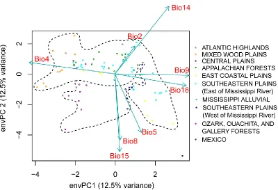
http://www.worldclim.org) reduced of collinearity (VIF < 10). Both predictors were incorporated into best multivariate model (based on AIC) to predict proportion of total sequences aligning uniquely to Discula destructiva (untransformed response) vs. either (C) mean temperature of month sampled or (B) envPC1. For prediction plots of the best

1 Chapter 1: Ecological genomics of local adaptation in Cornus florida L. by genotyping by

sequencing

Andrew L. Pais1, Ross W. Whetten2, and Qiu-Yun (Jenny) Xiang1

1

Department of Plant and Microbial Biology, North Carolina State University, Raleigh, NC 27695-7612

2

Department of Forestry, North Carolina State University, Raleigh NC 27695-8001

Published in Ecology and Evolution, available at

27 Chapter 2: Discovering variation of secondary metabolite diversity and its relationship with

disease resistance in Cornus florida L.

Andrew L. Pais1* (ALP), Xu (Sirius) Li1,2, and Qiu-Yun (Jenny) Xiang1

1

Department of Plant and Microbial Biology, North Carolina State University, Raleigh, NC 27695-7612

2

Plants for Human Health Institute, North Carolina State University, Kannapolis, NC 28081

Abstract

Understanding intraspecific relationships between genetic and functional diversity is a major goal in the field of evolutionary biology and is important for conserving biodiversity. Linking intraspecific molecular patterns of plants to ecological pressures and trait variation remains difficult due to environment-driven plasticity. Next-generation-sequencing,

untargeted LC-MS profiling, and interdisciplinary approaches integrating population genomics, metabolomics, and community ecology permit novel strategies to tackle this problem. We analyzed six natural populations of the disease-threatened Cornus florida L. from distinct ecological regions using genotype-by-sequencing markers and liquid

chromatography–mass spectrometry (LC-MS) based untargeted metabolite profiling. We tested the hypothesis that higher genetic diversity in C. florida yielded higher chemical diversity and less disease susceptibility (screening hypothesis) or if ecological factors induced the majority of chemical variation in plant response. We also determined if genetically similar subpopulations were similar in chemical composition. Lastly, we

29 association suggested that a putative iridoid glucoside was associated to SNPs under

selection.

Introduction

Plant secondary metabolites are closely tied to ecological functions and greatly affect community interactions (Dixon & Paiva 1995; Moore et al. 2014). Certain secondary

metabolites may provide plants with specialized functions like deterrence to herbivory or infection (Harborne & Turner 1984). Identifying the genetic basis of secondary compounds for such functions is of interest to the field of evolutionary ecology. Even small changes in genetic diversity may yield exceptionally large changes in secondary metabolism—

Secondary metabolite richness and relative abundance—referred to as

chemodiversity—are informative yet understudied metabolome properties helpful for understanding evolutionary and ecological processes (Hilker 2014; Kellerman et al. 2014). Promising work has investigated broader patterns of natural metabolome variation in the context of natural genetic variation. Significant correlations between metabolic and genetic distances were detected in nine Arabidopsis thaliana accessions exposed to different environments (Houshyani et al. 2012). Multi-generational lines inbred from different Drosophila melanogaster populations were found to remain distinguishable in general lipid composition, and approximately one fifth of the lipid compounds had clear concentration differences between male and female genotypes (Scheitz et al. 2013). In a more recent study, environmental and bud-leaf metabolome analyses of Pinus pinaster (ten European

provenances in common garden) revealed two distinct regional groups (Meijón et al. 2016). These researchers used distance measures based on a reduced-dimensionality of abundance differences for targeted compounds instead of explicitly calculating and comparing diversity indices (Appendix A), which account for both chemical compounds presence-absence and relative abundances within each sample.

31 al. 2013) with adoption of these chemical diversity indices would further demonstrate the power of this approach to understand the role genetics (i.e. locally adapted genes), plant functional diversity (i.e. chemodiversity), and environment play in influencing plant health.

We use a multidisciplinary approach to characterize and evaluate how properties of genetic diversity and chemodiversity contribute to susceptibility or resistance to disease in Cornus florida (L.), the flowering dogwood tree. This species naturally occurs throughout much of eastern North America and is ecologically important partly because of calcium it delivers to food chains in deciduous forests (Holzmueller et al. 2006; Baird 1980; Blair 1982; Linzey & Brecht 2003; Borer et al. 2013; Lovenshimer & Frick-Ruppert 2013). In addition, the plant is a cultural icon, serves as the emblem of three southern US states (Jordan 2010), and is valued in the horticulture industry at 30 million dollars in annual sales (NASS, USDA; 2007 Census of Agriculture). In the past three decades, C. florida populations have

experienced major declines in health due to the introduction of a fungal pathogen (Discula destructiva) to North America (Miller et al. 2016), the causal agent of dogwood anthracnose (Redlin 1991). Northern and montain populations have been hardest affected with up to 98% mortality occurring in monitored stands (Sherald et al. 1996; Hiers & Evans 1997; Williams & Moriarity 1999; McEwan et al. 2000; Rossell et al. 2001; Jenkins & White 2002). As dogwood anthracnose disease progresses southward along the Appalachian Mountains, populations of C. florida continue to decline (Jones et al. 2012). Whether or not the range of dogwood anthracnose (Fig. 2.1) will expand to the southeast overtime is uncertain.

evidence from multivariate analyses of flowering dogwood tree metabolomes, reduced genome sequences from genotype-by-sequencing (Peterson et al. 2012; Pais et al. 2016), and environmental data to address the following questions: (I) What is the relationship between genetic diversity and chemodiversity? (II) Is dogwood disease constrained primarily by abiotic factors? (III) Is there evidence from candidate SNPs and metabolites for local adaptation, and are there particular chemical biomarkers differentially expressed between diseased and healthy plants? (IV) Do healthy plants exhibit greater chemodiversity, and what environmental factors are inducing changes in chemodiversity the most?

Materials and Methods Plant material

Natural populations of C. florida were sampled from the mountain, Piedmont, and Coastal Plain regions of North Carolina during the summer of 2012 (Pais et al. 2016). Each region contained two populations, and each population consisted of one or two collection sites, or subpopulations, of 30 to 15 individual trees respectively, for a total of 180 mature and unique trees. Leaves were dried and stored in silica gel under standardized conditions. All samples were given an extended period to dry before extracting thermally stable metabolites from leaves.

Metabolite extraction

33 to avoid sampling metabolites unique to fungi. During the drying period, eight samples developed mold growth, which prohibited their use for metabolic study—leaving 172 remaining samples. Leaf tissue was ground with liquid nitrogen in a Retsch MM 400 oscillating mill for one min at 25 Hz. After grinding, two ml of 50% methanol were

immediately applied to samples. Samples were then incubated in a water bath for 30 min at 60oC and allowed to cool one hour at 4oC to minimize potential precipitate (soluble in warm solution) from being transferred to final vials. After centrifuging for one min, remaining supernatant was transferred to a new vial via a filtered syringe tube.

Untargeted metabolite profiling

LC-MS data processing

Raw data files obtained from LC-MS experiments were converted to the mzData format using Agilent Masshunter software, grouped into directories by population, and then uploaded to the XCMS Online platform (Tautenhahn et al. 2012) for automatic metabolite detection and alignment. Metabolite features—peaks defined by mass-to-charge ratio (m/z), retention time (RT), and intensity—were extracted with optimized parameters: centWave method, minimum-maximum peak width = 8 and 30, signal to noise threshold = 30, mzdiff = 0.01, prefilter peaks = 3, prefilter intensity = 2000, and noise filter = 0. Since retention time variation between runs was minimal, the peaks were aligned across all the samples without RT correction, using the following parameters: bw = 5, mzwid = 0.025, and minfrac = 0.75. A list of 2,785 aligned peaks/features from 172 individuals was then exported from XCMS Online as a tab separated file. A preliminary PCA using auto-scaled distances of individual peak areas and a distance to model (DModX) test (implemented in XCMS) detected

35 Chemodiversity index calculation

We calculated six diversity indices (Appendix A), similarly adopted for metabolic analyses in Morris et al. (2014), using R packages vegan (Oksanen et al. 2016) and

BiodiversityR (Kindt 2016). Calculation of the richness diversity index (S; Whittaker 1972) is primarily described in this study since its results have straightforward and biologically-meaningful interpretations, which can be easily re-conceptualized from the study of species diversity to the study of chemodiversity. Since several different diversity indices may be useful as indicators of biodiversity (Hurlbert 1971) and chemodiversity (Morris et al. 2014), Appendix A provides detailed calculations, explanations, and results for the remaining five diversity indices [Shannon’s index (H’; Shannon 1948), Simpson’s index of diversity (D1; McCune & Grace 2002), Simpson’s inverse or dominance index (D2; McCune & Grace 2002), Evenness (E), and Berger-Parker’s dominance index (BP; Berger & Parker 1970)].

α-richness (Whittaker 1972). In contrast, γ-α-richness assesses total number of unique

metabolites within a given subpopulation. Since exploratory findings showed that γ-richness was equal among subpopulations, we hereinafter refer to α-richness when reporting chemical richness.

Genetic marker data

To examine chemical-genotype associations, we first used genotype-by-sequencing (GBS; Peterson et al. 2012) of two Illumina Hiseq libraries, de novo assembly into 90 bp GBS tags with STACKS (Catchen et al. 2011), latent factor mixed modeling [a genotype-environment association (GEA) method; Frichot et al. 2013], and two Fst outlier methods (Foll & Gaggiotti 2008; Excoffier et al. 2009) to classify putatively neutral SNPS and SNPs exhibiting varying support for being under selection (Pais et al. 2016). Putatively neutral reference SNPs were used to calculate marker-based inbreeding coefficients (F; Keller et al. 2011) and identity-by-state matrices using PLINK (Purcell et al. 2007). We added an

inbreeding coefficient (F) variable into logistic models characterizing plant health and disease (see details below) because we recognized that greater heterozygosity (fewer

homozygous loci than expected) within an individual could affect plant health (Ouborg et al. 2000) by yielding more unique metabolites and raising plant potential to respond to novel pathogen effectors (screening hypothesis; Jones et al. 1991). GBS samples were also

37 Environmental-functional traits

We correlated climate-soil variables (obtained through collection site measurements and GIS extrapolation; Pais et al. 2016) and temperature-precipitation estimates at time of collection (daily-monthly; PRISM Climate Group; extracted 30 Jan 2015) with

chemodiversity indices (Table 2.1). Similarly, plant health scores were plotted against chemodiversity levels. Visual health-disease estimates were taken using the procedure of Mielke & Langdon (1986) based on the percent of tree canopy affected by leaf blotting, necrosis, or branch dieback. Additionally, five categorical scores obtained from this method were converted into a binary variable. Plants with scores of four and five were considered healthy while plants with scores of three and below were considered diseased. This recoded binary variable served as the response for mixed model logistic regressions. For further description how environmental variables were selected for multivariate modeling of

chemodiversity levels, see Appendix A and additional justification of mixed logistic models as described further in methods.

Characterizing general relationships of chemical structure and diversity to plant health and genetic diversity

components (PC) to maximize among-population variation and minimize within-population variation. We estimated and analyzed PC scores separately from two different datasets (both scaled): reference SNPs aligning to the C. florida draft genome and abundance data (log-transformed) for 377 metabolites. We conducted DAPC both by defining groups by collection sites and by allowing the program clustering algorithm to find optimal cluster number (K) without priors. DAPC does not require assumptions on a population genetic model (e.g. linkage equilibrium of markers) in contrast to programs like STRUCTURE (Pritchard et al. 2000) so DAPC has been widely adopted in recent population genetic studies (Grünwald & Goss 2011; Buchalski et al. 2016; Cahill & Levinton 2016). Its use for

metabolic study is recent, but its efficacy in discriminating different biologically meaningful chemotype classes has been demonstrated and favored over other discriminant analysis methods under certain circumstances (Scheitz et al. 2013; Gromski et al. 2015).

Next, we estimated average genetic diversity and chemodiversity of each

39 derived from 377 metabolites (or all 2,785 chemical features to better compare between-sample differences) were calculated per between-sample and averaged by subpopulation for

correlation analyses, and subpopulations were compared with 95% confidence intervals for each genetic-chemical diversity estimate.

We next tested for correlations between environmental gradients, genetic differentiation, and chemical distance using Mantel tests and linear regression. Full and partial Mantel tests (Legendre & Fortin 1989) were implemented in the R package ecodist (Goslee 2007) with 9,999 permutations and 500 bootstraps to determine the strength and significance of association between population-level metabolic distance, genetic distance, and mean euclidean distances of spatial and environmental variables [i.e. displacement of collection sites, precipitation of driest month (Bio14), and temperature at day of collection (Tcol); see Environmental-functional traits continued in Appendix A for justification of environmental variables tested]. For these correlation analyses, we employed Arlequin (Excoffier & Lischer 2010) and reference SNPs (putatively neutral SNPs from Pais et al. 2016) to create a matrix of linearized Fst values between subpopulations. We then correlated this Fst matrix to an analogous matrix describing population similarities and dissimilarities using metabolite data. To compare metabolic distances between subpopulations, we

constructed an ANOSIM (Analysis of Similarities) R matrix from inter-sample euclidean distances following the approach of Houshyani et al. (2012) and Kabouw et al. (2009), 377 log-transformed metabolites, and the program PAST (Hammer et al. 2001). An ANOSIM matrix is a reduced-dimension matrix describing the similarity between pairs of

the Fst matrix to the ANOSIM R matrix of population-level metabolic distances were assessed using one-tailed Mantel tests of Pearson’s r coefficient.

The significance of simple linear regressions between individual-specific

chemodiversity levels, inbreeding coefficients, and all available environmental predictors was also assessed. In addition, we determined the best multivariate models describing general chemodiversity as the response (Appendix A). For these initial regression models, we used chemodiversity indices based on all 2,785 chemical features as this allowed us to more reliably detect differences in chemical richness among samples.

Biomarker analyses

For identifying biomarkers associated with healthy vs. diseased trees, we used random forests (RF), DAPC, partial least squares discriminant analysis (PLS-DA), support vector machines (SVM), and a logistic mixed model predicting disease states based on abundance of each metabolite (latter model controlling for inbreeding coefficient,

41 Predicting metabolite-SNP networks

To understand patterns between chemical data and individual loci while controlling for sample structure and environmental variability, we employed a linear mixed model implemented in EMMAX (Kang et al. 2010). This model has been used in genome-wide-association (GWA) studies of Arabidopsis thaliana (Li et al. 2010; Fournier-Level et al. 2011;Li et al. 2014; Bac-Molenaar et al. 2015; Strauch et al. 2015)because of its

computational efficiency and ability to handle population stratification (Price et al. 2010). We corrected for population structure by entering an identity-by-state matrix (created from neutral reference SNPs to describe pairwise relationships between individuals) into our model. For SNP association, we log-transformed metabolite abundances prior to association study. For each corresponding GBS tag of a SNP, we noted any BLAST result, gene

annotation (SWISS-PROT, TAIR, or UNI-PROT), and alignment match to the transcriptome (Zhang et al. 2013) or draft genome of C. florida.

Chemical-genotype associations were calculated in EMMAX with: (1) no covariates present; (2) the Bio14 covariate present; (3) the Tcol covariate present; or (4) both covariates present (see Environmental-functional traits continued in Appendix A for justification of covariates specified). P-value distributions from output files were plotted using R package Haplin (Wilcox et al. 1998) to assess Q-Q plots for each metabolite. Results were considered significant for genotype-metabolite associations passing a Bonferroni correction with an alpha value of 5%. Only results from normally distributed Q-Q plots were considered.

coefficients to test for correlation between two metabolites while removing other metabolite effects. Justifications and additional considerations of GGM are further discussed in

Appendix A (Gaussian graphical modelling continued).

Modeling health vs. disease: logistic mixed modelling with chemodiversity of a specific set of biomarkers

43 collection, we consistently found the interaction effects to be insignificant. The same applied when testing interactions to inbreeding coefficient. Thus, we removed interaction terms from our models.

Results

Genetic markers

Of 1,631 GBS tags (containing 2,118 SNPs) consistently genotyped from two Hiseq libraries in Pais et al. (2016), we selected 1,860 SNPs for studying chemical-genotype associations. These SNPs passed a 5% minor allele frequency filter, a locus genotyping rate in 80% or greater of all samples, and Hardy-Weinberg exact tests implemented in Genepop (Rousset 2008) indicating allele equilibrium in over half of subpopulations. We selected one SNP per GBS tag to reduce linkage disequilibrium in our dataset, parsing final SNP number to 1,446. For GBS tags showing no evidence of being under selection from Pais et al. (2016), SNPs occurring closest to the PstI cut-site were selected, leading to 1,171 SNPs as the

neutral reference. For GBS tags showing any evidence of being under selection (Pais et al. 2016), SNPs with the highest estimated Fst were included in the 1,446 SNP dataset for GWA to metabolites. Of those 1,446 SNPs, 1,163 SNPs occurred within GBS-tags aligning to the C. florida draft genome and were applied to DAPC analyses.

General patterns of chemical-genetic structure and diversity

but subsequent comparisons of rarefied-allelic richness showed that Piedmont subpopulations had higher mean rarefied-allelic richness than mountain and coastal subpopulations—

especially in comparison to mountain subpopulation SM2, which had the lowest rarefied-allelic richness (Fig. 2.2D); contrasts of chemodiversity between subpopulations were most apparent for richness measures—with mountain subpopulations SM1 and SM2 having significantly lower chemical richness on average compared to Piedmont and coastal subpopulations (Fig. 2.2F and G; see Fig. A.2 for subpopulation means of other

chemodiversity indices). Levels of rarefied-allelic richness and chemical richness were similar and significant correlations between subpopulation means were observed (Fig. 2.2G). When grouping individual trees into healthy or diseased categories based on a one to five scoring system (Mielke & Langdon 1986), the relationship of disease status to

chemodiversity indices (derived from either 377 metabolites or all 2,785 chemical features) varied depending on the index (Fig. A.3). In particular, chemodiversity measured by richness highly overlapped among the five disease-state groups (Fig. 2.3), but showed slight trends of chemodiversity medians increasing with increasing health states of individual trees,

especially for chemical richness of the 377 metabolites (Fig. 2.3A).

45 subpopulations, DAPC using genetic distances only supported two clusters—one cluster consisting of samples from mountain-Piedmont ecoregions and another cluster consisting of samples from the Coastal Plains ecoregion (Pais et al. 2016; Fig. 2.4C and Fig. 2.4E). In contrast, DAPC for metabolite data (without restricting samples to group by sampling location) supported up to seven clusters related to geography and conditions at collection sites (Fig. 2.4D and Fig. 2.4F). Clusters with high membership of mountain individuals (i.e. cluster seven and three) were located in the upper ordination space while cluster five

(consisting of individuals primarily from the coast) and cluster four (including Piedmont samples and samples from the PI mountain subpopulation) were located lower along the ordination space (Fig. 2.4F). Cluster one had relatively few coastal individuals; cluster six included no members of the SM mountain subpopulations; and cluster seven consisted primarily of SM mountain samples (Fig. 2.4D).

Mantel test results showed strong collinearity between site-specific effects on chemical differences between subpopulations (Table 2.2). Isolation by distance tests using either genetic distances or metabolic distances for Mantel tests were both significant (r > 0.5 and p < 0.05). The relationship between metabolic distance and genetic distances of

When analyzing environmental predictors in simple linear regression, several predictors had significant correlations to at least three or more chemodiversity indices

derived from 2,785 chemical features (Fig. A.4). Such predictors were considered in variable selection for best multivariate models describing general chemodiversity. Our best

multivariate model indicated that higher inbreeding coefficients in individuals were

predictive of smaller chemical richness after controlling for other abiotic effects (Estimate = -47.276 chemical features, p = 0.007; Fig. A.5). Supplementary results of simple linear regressions and other multivariate models are presented in Table A.1 and Table A.2.

Candidate metabolite-SNP network

To understand the connections between genetic polymorphism and metabolite variation, we performed GWA analyses on the 2,785 features of 377 metabolites. With and without covariates, we identified 975 unique chemical features significantly associated with 347 unique SNPs. Overlapping chemical feature and SNP results among the various GWA tests (different covariates specified) are presented in Fig. 2.5 and summarized here

47 of similarities and differences in results among the various covariate-dependent GWA tests for all chemical features and SNPs available in Appendix A.

We performed GGM to construct metabolite networks based on partial correlation. This analysis, combined with the GWA results, revealed SNP-metabolite connections for a putative terpenoid glucoside network (Fig. 2.6A). We noted GGM connections of three metabolites consisting of an annotated iridoid glucoside/Eleganoside C (M435T576; Bailleul et al. 1981; Ali et al. 2000; Xu et al. 2008), an aglycone/Cornolactone C (M227T630; He et al. 2014), and a possible intermediate (M451T432). Moreover, several SNPs were repeatedly found to be significantly associated with chemical features of these three metabolites (Fig. 2.6A). SNP loci with multiple significant associations (labelled yellow; Fig. 2.6) within this network were: B506_11, B1401_69 (aligned to gene encoding for oligomeric Golgi complex; Ostertag et al. 2013), B447_54, B977_86, B982_75 (aligned to gene encoding for lectin-domain receptor kinase; Singh & Zimmerli 2013), B536_31, B1327_41, and B440_76 (aligned to gene encoding for a protein sensitive to rhizotoxicity; Sawaki et al. 2009; Fan et al. 2016). Several of these SNPs (B1401, B982_75, B440_76, B1401_69, B447_54, and B977_86) also showed evidence of being under selection in Pais et al. (2016).

Predicting disease status from metabolite markers

were few overlaps between the biomarkers detected by different methods (Fig. A.7A). Logistic mixed modeling of individual metabolites showed that six metabolites were significantly correlated with the log odds of being healthy vs. diseased (Table 2.3) after controlling for temperature at collection, inbreeding coefficient, and collection site random effects. Out of the 39 biomarker metabolites, five had significant associations with SNPs as revealed from GWA analysis (Fig. A.7A). The hypothesized networks for these metabolites constructed from GWA and GGM results were shown in Fig. 2.6 and Fig. A.8.

49 Ten other credible biomarkers not involved exclusively in the hypothesized glycoside network were shown to be strongly associated with plant disease status (Fig. A.6; Fig. A.7). Accumulations of these ten metabolites (including M435T576) were highly predictive of plant health and disease status, according to multiple biomarker test results (Fig. A.7). Chemodiversity patterns derived from these ten biomarkers also showed that the dominance of M435T576 (in relation to the relatively even expression of other biomarkers) was

associated with log odds of a plant being healthy vs. diseased (Table A.3; Appendix A; Other candidate biomarkers continued).

Discussion

Relationships of genetic diversity and chemodiversity

flavonoids, phenolics, terpenoids, etc. (Appendix A). Our analysis showed largely

concordant chemical-genetic distance clustering patterns (Fig. 2.4). For instance, mountain subpopulations (cooler in temperature and with higher disease severity) exhibited distinct chemical profiles and clustered together as in genetic analyses (excluding PI1), and two studied mountain subpopulations were lower in both metabolite richness (Fig. 2.2F and G) and genetic diversity (rarefied-allelic richness) than the studied Piedmont subpopulations (Fig. 2.2D). Moreover, trees with greater individual-level heterozygosity (i.e. smaller inbreeding coefficients) showed greater chemical α-richness after controlling for other abiotic effects (Fig. A.5). While chemical richness of 377 metabolites was not significantly correlated with means of allelic richness across subpopulations (r2 = 0.2017, p = 0.2643), a positive correlation between subpopulation means of rarefied-allelic richness and chemical α-richness of all 2,785 chemical features was detected (p = 0.05587; Fig. 2.2H). These findings suggest that chemical variation preserved in dried leaves may have a link to genetic variation and functional diversity within a species.

There is clear impetus to conserve genetically and chemically diverse plant

populations. It has been demonstrated that even small differences in genetic diversity (such as single amino acid substitutions) can yield large differences in chemical profiles

(Kampranis et al. 2007), and several studies have found that higher intraspecific genetic diversity reduces herbivory and disease in plant populations (Hughes et al. 2008). Moreover, emerging evidence has demonstrated how variation in intraspecific chemodiversity

51 between clustering patterns derived from genetic and metabolite data in addition to noting evidence that some diseased mountain subpopulations (Fig. 2.1; Fig. A.1) have lower genetic and chemical diversity. Namely, these findings suggest that genetic variation in conjunction with environment entails chemical variation, which indirectly influences plant robustness to environmental stress. Thus, there is probable disease-related differentiation in genetics and metabolites for these natural populations. This relationship between genetic diversity and chemodiversity found in C. florida validates promising efforts to conserve functional diversity (i.e. chemodiversity) by prioritizing genetic diversity.

Environmental and genetic factors on disease

One of the goals of this study is to gain insights into the question whether

(sampled in this study; Fig. 2.1, Fig. A.1). These observations (or lack thereof) suggest disease may be primarily affected by abiotic factors.

However, as previously discussed, C. florida also exhibits a gradient of variation in genetics and metabolites among North Carolina’s coast, Piedmont, and mountain ecoregions (Fig. 2.2; Fig. 2.4; Fig. A.1), which corresponds to a variation in health scores (Fig. A.1; Fig. A.4; Pais et al. 2016). Furthermore, relatively high chemodiversity estimates among 377 metabolites or all 2,785 chemical features are observed in healthier plants (Fig. 2.3; Fig. A.3). Since healthy plants occur in all environments from the Coastal Plains to mountains, this finding suggests that dogwood anthracnose may not necessarily be constrained by only abiotic factors (e.g. cooler and moister habitats) but instead may also be affected by both genetic and metabolite diversities. Genetic and metabolite diversity may be important to disease variation. High levels of metabolic and genetic diversity intrinsic to the host may benefit individual trees in staving off disease infection (Jones & Firn 1991). Alternatively, low genetic diversity in mountain populations can also be a consequence of dogwood anthracnose disease effects (Hadziabdic et al. 2012). Although the co-occurrence of these patterns in C. florida presents challenges to distinguish relative roles of abiotic, genetic, and chemical factors, available evidence supports an influence of genetics on disease as

elaborated below.

Previous ecological genomic analysis using GBS data (Pais et al. 2016) has identified SNPs under selection for local adaption in the species, and a few of these SNPs are

53 genes associated with plant-chemical responses to disease pressure after controlling for environment. SNP loci B1401, B982_75, B440_76, B1401_69, B447_54, and B977_86 [previously identified to be under selection in Pais et al. (2016)] were found to be associated with a notable iridoid glucoside that was identified as a positive RF biomarker of health vs. disease (M435T576; Fig. 2.6; Fig. 2.8; Fig. A.6; Fig. A.7). Several of these candidate SNPs occurred on loci with predicted functions related to disease resistance. Some SNP loci such as B1401 may encode for proteins (i.e. an oligomeric Golgi complex) that facilitate

glycosylation to inhibit disease (Ostertag et al. 2013). Other loci such as Fst outlier B982 (Pais et al. 2016) are predicted to encode for signaling receptors like lectin-domain receptor kinases, which have been previously implicated in plant immunity responses among other signaling processes (Singh & Zimmerli 2013), and recent functional experimentation on resistance genes encoding for such receptors in Solanaceous plants has provided evidence for Phtophthora resistance (Wang et al. 2015). Other SNP loci like B440 may encode regulatory proteins (Sawaki et al. 2009; Fan et al. 2016), which similarly respond to stress by regulating transcription of genes involved in pathways such as immunity response. Biomarker

It must be stated that candidate SNPs and biomarkers identified in our analyses require additional resources and work to validate their chemical identities, but these

unverified chemical compounds serve as an important guide for prioritizing which SNPs and biomarkers to further test in future research. The abundance and inducibility of certain secondary metabolites such as flavonoids, other phenolics, and glycoside derivatives have been found to be heritable and mediated by herbivore-pathogen pressures (Johnson et al. 2009; Li et al. 2014). Determining the specific genetic factors regulating such adaptive metabolites remains an important goal, and this study adds to emerging efforts to integrate large secondary metabolite concentration data with information from genome scans (Eckert et al. 2012; Jensen et al. 2016; Talbot et al. 2016).

Herbivore/pathogen interactions influencing chemodiversity in plants

Explanations for natural variation of secondary metabolism have long been debated (Fraenkel 1959). Intraspecific variation of plant chemodiversity can be attributed to

55 sesquiterpene lactone diversity (herbivory deterrent) in populations further away from the equator, which was explained as a result of selection for lower toxicity due to fewer

herbivore-plant interactions in areas far from the equator (Salazar & Marquis 2012; Aráoz et al. 2016). This variation of sesquiterpene lactone diversity in the species may well have a genetic basis, which has not been investigated. In C. florida, a subset of the species

distribution occurs from the southern Appalachians to southeastern Coastal Plains where an elevational-temperature gradient spans eastward through the Piedmont, and we have found a decreasing trend of chemodiversity and genetic diversity in subpopulations more embedded in the Appalachian Mountains (Fig. 2.2D, F, and G). While lower temperatures may possibly be related to lower secondary plant metabolism of trees in the mountains, lower

chemodiversity levels in mountain populations may be a result of lower genetic variation or a consequence of the disease infection, as mountain populations are in general less healthy. While diseased plants may show deficiencies in metabolism due to necrosis, our standardized method for extracting visibly unaffected tissue from both diseased and healthy plants makes the infection scenario less likely. The less healthy plants may possess genotypes that mediate metabolism of biosynthetic pathways in ways contributing to less constitutively expressed products— increasing plant susceptibility to initial infections. Higher genetic diversity in certain individuals (e.g. less homozygous genotypes; Fig. A.5) or subpopulations (e.g. higher rarefied-allelic richness; Fig. 2.2D) can confer a greater range of gene products (e.g.

On the other hand, herbivory and infection on plants can also induce greater

57 Conclusions

Our study demonstrates untargeted metabolite profiling is a useful tool for understanding biodiversity in a new dimension. Secondary metabolites preserved in C. florida dried leaves from natural populations provided data for evaluating chemodiversity and identifying potential disease biomarkers. We found congruent patterns of chemical and genetic variation and identified several biomarkers indicative of disease and health. From those results, a select candidate SNP-metabolite group (i.e. iridoid glucosides) of clear ecological importance was identified to guide future study. Additional investigation of chemical diversity with increased sampling across the species range may provide more details on the relationship among genetics, metabolites, and dogwood anthracnose in C. florida, which in turn may shed light on forest diseases in general.

Acknowledgements

References

Ali MS, Uzair SS, Krebs HC, Jahangir M, Habermehl GG (2000) Eleganoside-A, B and C from Pseudocalymma elegans, a native of Brazil. Phytochemistry, 55, 359-362.

Alonso A, Marsal S, Julià A (2015) Analytical methods in untargeted metabolomics: state of the art in 2015. Frontiers in bioengineering and biotechnology, 3.

Anderson JT, Willis JH, Mitchell-Olds T (2011) Evolutionary genetics of plant adaptation. Trends in Genetics, 27, 258-266.

Aráoz MVC, Mercado MI, Grau A, Catalán CA (2016) Intraspecific variation of

sesquiterpene lactones associated to a latitudinal gradient in Smallanthus macroscyphus (Heliantheae: Asteraceae). Chemoecology, 1-9.

Bac-Molenaar JA, Fradin EF, Rienstra JA, Vreugdenhil D, Keurentjes JJ (2015) GWA Mapping of Anthocyanin Accumulation Reveals Balancing Selection of MYB90 in Arabidopsis thaliana. PloS one, 10, e0143212.

Bailleul F, Leveau AM, Durand M (1981) Nouvel Iridoide des Fruits de Lonicera alpigena. Journal of Natural Products 44 (5), 573-575.

Baird NA, Etter PD, Atwood TS, et al (2008) Rapid SNP discovery and genetic mapping using sequenced RAD markers. PloS one, 3, e3376.

Baldwin IT, Halitschke R, Kessler A, Schittko U (2001) Merging molecular and ecological approaches in plant–insect interactions. Current opinion in plant biology, 4, 351-358.

Barbosa P, Hines J, Kaplan I, Martinson H, Szczepaniec A, Szendrei Z (2009) Associational resistance and associational susceptibility: having right or wrong neighbors. Annual review of ecology, evolution, and systematics, 40, 1-20.

Bartel J, Krumsiek J, Theis FJ (2013) Statistical methods for the analysis of high-throughput metabolomics data. Computational and structural biotechnology journal, 4, 1-9.

Bartsch M, Bednarek P, Vivancos PD, et al (2010) Accumulation of isochorismate-derived 2,3-dihydroxybenzoic 3-O-beta-D-xyloside in arabidopsis resistance to pathogens and ageing of leaves. The Journal of biological chemistry, 285, 25654-25665.

Benard C, Bernillon S, Biais B, et al (2015) Metabolomic profiling in tomato reveals diel compositional changes in fruit affected by source-sink relationships. Journal of experimental botany, 66, 3391-3404.

59 Blair RM (1982) Growth and nonstructural carbohydrate content of southern browse species as influenced by light intensity. Journal of Range Management, 756-760.

Bolnick DI, Amarasekare P, Araújo MS, et al (2011) Why intraspecific trait variation matters in community ecology. Trends in ecology & evolution, 26, 183-192.

Borer CH, Sapp SG, Hutchinson LH (2013) Flowering dogwood (Cornus florida L.) as mediator of calcium cycling: new insights are revealed by analysis of foliar partitioning. Trees, 27, 841-849.

Buchalski MR, Sacks BN, Gille DA, et al (2016) Phylogeographic and population genetic structure of bighorn sheep (Ovis canadensis) in North American deserts. Journal of mammalogy, gyw011.

Cahill AE, Levinton JS (2016) Genetic differentiation and reduced genetic diversity at the northern range edge of two species with different dispersal modes. Molecular ecology, 25, 515-526.

Calcagno V (2013) glmulti: Model selection and multimodel inference made easy. R package version, 1.

Caplan J, Padmanabhan M, Dinesh-Kumar SP (2008) Plant NB-LRR immune receptors: from recognition to transcriptional reprogramming. Cell host & microbe, 3, 126-135.

Caspi R, Altman T, Billington R, et al (2014) The MetaCyc database of metabolic pathways and enzymes and the BioCyc collection of Pathway/Genome Databases. Nucleic acids research, 42, D459-D471.

Catchen JM, Amores A, Hohenlohe P, Cresko W, Postlethwait JH (2011) Stacks: building and genotyping loci de novo from short-read sequences. G3: Genes, Genomes, Genetics, 1, 171-182.

Chambers MC, Maclean B, Burke R, et al (2012) A cross-platform toolkit for mass spectrometry and proteomics. Nature biotechnology, 30, 918-920.

Chang J, Xuan L, Xu Y, Zhang J (2001) Seven new sesquiterpene glycosides from the root bark of Dictamnus dasycarpus. Journal of natural products, 64, 935-938.

Eckert AJ, Wegrzyn JL, Cumbie WP, et al (2012) Association genetics of the loblolly pine (Pinus taeda, Pinaceae) metabolome. New Phytologist, 193, 890-902.

Ennos RA (2015) Resilience of forests to pathogens: an evolutionary ecology perspective. Forestry, 88, 41-52.

Excoffier L, Hofer T, Foll M (2009) Detecting loci under selection in a hierarchically structured population. Heredity, 103, 285-298.

Excoffier L, Lischer HE (2010) Arlequin suite ver 3.5: a new series of programs to perform population genetics analyses under Linux and Windows. Molecular ecology resources, 10, 564-567.

Fraenkel GS (1959) The raison d'etre of secondary plant substances. Science, 129, 1466-1470.

Fan W, Lou HQ, Yang JL, Zheng SJ (2016) The roles of STOP1-like transcription factors in aluminum and proton tolerance. Plant signaling & behavior, 11, e1131371.

Firn RD, Jones CG (2000) The evolution of secondary metabolism–a unifying model. Molecular microbiology, 37, 989-994.

Foll M, Gaggiotti O (2008) A genome-scan method to identify selected loci appropriate for both dominant and codominant markers: a Bayesian perspective. Genetics, 180, 977-993. Fournier-Level A, Korte A, Cooper MD, Nordborg M, Schmitt J, Wilczek AM (2011) A map of local adaptation in Arabidopsis thaliana. Science, 334, 86-89.

Frichot E, Schoville SD, Bouchard G, François O (2013) Testing for associations between loci and environmental gradients using latent factor mixed models. Molecular biology and evolution, 30, 1687-1699.

Glassmire AE, Jeffrey CS, Forister ML, et al (2016) Intraspecific phytochemical variation shapes community and population structure for specialist caterpillars. New Phytologist. Gomez-Casati DF, Zanor MI, Busi MV (2013) Metabolomics in plants and humans: applications in the prevention and diagnosis of diseases. BioMed research international, 2013.

Goslee SC, Urban DL (2007) The ecodist package for dissimilarity-based analysis of ecological data. Journal of Statistical Software, 22, 1-19.

61 Gromski PS, Muhamadali H, Ellis DI, et al (2015) A tutorial review: Metabolomics and partial least squares-discriminant analysis–a marriage of convenience or a shotgun wedding. Analytica Chimica Acta, 879, 10-23.

Grünwald NJ, Goss EM (2011) Evolution and population genetics of exotic and re-emerging pathogens: novel tools and approaches. Annual Review of Phytopathology, 49, 249-267. Hadziabdic D, Wang X, Wadl PA, Rinehart TA, Ownley BH, Trigiano RN (2012) Genetic diversity of flowering dogwood in the Great Smoky Mountains National Park. Tree genetics & genomes, 8, 855-871.

Hammer Ø, Harper D, Ryan P (2001) PAST: Paleontological Statistics Software Package for education and data analysis.Palaeontolia Electronica 4.

Harborne JB, Turner BL, Harborne J (1984) Plant chemosystematics.

He Y, Peng J, Hamann MT, West LM (2014) An iridoid glucoside and the related aglycones from Cornus florida. Journal of natural products, 77, 2138-2143.

Hiers JK, Evans JP (1997) Effects of anthracnose on dogwood mortality and forest composition of the Cumberland Plateau (USA). Conservation Biology, 11, 1430-1435. Hilker M (2014) New synthesis: parallels between biodiversity and chemodiversity. Journal of chemical ecology, 40, 225.

Hill MO (1973) Diversity and evenness: a unifying notation and its consequences. Ecology, 54, 427-432.

Holzmueller E, Jose S, Jenkins M, Camp A, Long A (2006) Dogwood anthracnose in eastern hardwood forests: what is known and what can be done? Journal of Forestry, 104, 21-26. Houshyani B, Kabouw P, Muth D, de Vos RC, Bino RJ, Bouwmeester HJ (2012)

Characterization of the natural variation in Arabidopsis thaliana metabolome by the analysis of metabolic distance. Metabolomics, 8, 131-145.

Hughes AR, Inouye BD, Johnson MT, Underwood N, Vellend M (2008) Ecological consequences of genetic diversity. Ecology Letters, 11, 609-623.

Hurlbert SH (1971) The nonconcept of species diversity: a critique and alternative parameters. Ecology, 52, 577-586.

Jenkins MA, White PS (2002) Cornus florida L. mortality and understory composition changes in western Great Smoky Mountains National Park. Journal of the Torrey Botanical Society, 194-206.

Johnson MT, Agrawal AA, Maron JL, SALMINEN J (2009) Heritability, covariation and natural selection on 24 traits of common evening primrose (Oenothera biennis) from a field experiment. Journal of Evolutionary Biology, 22, 1295-1307.

Jombart T (2008) adegenet: a R package for the multivariate analysis of genetic markers. Bioinformatics, 24, 1403-1405.

Jombart T, Devillard S, Balloux F (2010) Discriminant analysis of principal components: a new method for the analysis of genetically structured populations. BMC genetics, 11, 1. Jones CG, Firn RD, Malcolm S (1991) On the evolution of plant secondary chemical diversity [and discussion]. Philosophical Transactions of the Royal Society of London B: Biological Sciences, 333, 273-280.

Jones WE, Smith WD, Twardus DB (2012) Tracking population loss in Cornus florida since discovery of Discula destructiva, causal agent of dogwood anthracnose, in eastern North America.

Jordan R. State Tree and State Flowers. State Tree and Flower. The United States National Arboretum, 14 July 2010. Web. 7 June 2016

Kabouw P, Biere A, van der Putten, Wim H, van Dam NM (2009) Intra-specific differences in root and shoot glucosinolate profiles among white cabbage (Brassica oleracea var.

capitata) cultivars. Journal of Agricultural and Food Chemistry, 58, 411-417.

Kampranis SC, Ioannidis D, Purvis A, et al (2007) Rational conversion of substrate and product specificity in a Salvia monoterpene synthase: structural insights into the evolution of terpene synthase function. The Plant Cell, 19, 1994-2005.

Kang HM, Sul JH, Service SK, et al (2010) Variance component model to account for sample structure in genome-wide association studies. Nature genetics, 42, 348-354. Keller MC, Visscher PM, Goddard ME (2011) Quantification of inbreeding due to distant ancestors and its detection using dense single nucleotide polymorphism data. Genetics, 189, 237-249.

Kellerman AM, Dittmar T, Kothawala DN, Tranvik LJ (2014) Chemodiversity of dissolved organic matter in lakes driven by climate and hydrology. Nature communications, 5.

Kindt R, Kindt MR (2016) Package ‘BiodiversityR’.

63 Krumsiek J, Suhre K, Illig T, Adamski J, Theis FJ (2011) Gaussian graphical modeling reconstructs pathway reactions from high-throughput metabolomics data. BMC systems biology, 5, 1.

Legendre P, Fortin MJ (1989) Spatial pattern and ecological analysis. Vegetatio, 80, 107-138.

Li X, Svedin E, Mo H, Atwell S, Dilkes BP, Chapple C (2014) Exploiting natural variation of secondary metabolism identifies a gene controlling the glycosylation diversity of

dihydroxybenzoic acids in Arabidopsis thaliana. Genetics,198, 1267-1276.

Li Y, Huang Y, Bergelson J, Nordborg M, Borevitz JO (2010) Association mapping of local climate-sensitive quantitative trait loci in Arabidopsis thaliana. Proceedings of the National Academy of Sciences, 107, 21199-21204.

Linzey D, Brecht C (2003) American beavers (Castor canadensis)—biodiversity of Great Smoky Mountains National Park. Discover Life in America, Gatlinburg, Tennessee, 37738. Lovenshimer J, Frick-Ruppert J (2013) Nutritional values of six native and introduced fall-ripening fruit species in western North Carolina. BIOS, 84, 218-226.

Marak HB, Biere A, Van Damme JM (2002) Systemic, genotype-specific induction of two herbivore-deterrent iridoid glycosides in Plantago lanceolata L. in response to fungal infection by Diaporthe adunca (Rob.) Niessel. Journal of chemical ecology, 28, 2429-2448. McCune B, Grace JB, Urban DL (2002) Analysis of ecological communities.

McEwan R, Muller R, Arthur M, Housman H (2000) Temporal and ecological patterns of flowering dogwood mortality in the mixed mesophytic forest of eastern Kentucky. Journal of the Torrey Botanical Society, 221-229.

Meijón M, Feito I, Oravec M, et al (2016) Exploring natural variation of Pinus pinaster Aiton using metabolomics: Is it possible to identify the region of origin of a pine from its

metabolites? Molecular ecology.

Meng J, Lu H, Li H, Yang L, Tan R (1999) A new antibacterial sesquiterpene glycoside and other bioactive compounds from Biebersteinia heterostemon. Spectroscopy Letters, 32, 1005-1012.

Mielke M, Langdon K (1986) Dogwood anthracnose fungus threatens Catoctin Mountain Park. Park Science, 6.