Multi-Level Reduced Order Modeling Equipped with Probabilistic Error Bounds.

(1)

ABSTRACT

ABDO, MOHAMMAD GAMAL MOHAMMAD MOSTAFA. Multi-Level Reduced Order Modeling Equipped with Probabilistic Error Bounds. (Under the direction of Hany S. Abdel-Khalik, Dmitriy Y. Anistratov, Ilse C. F. Ipsen and Ralph C. Smith).

Over the past few decades, engineering analysts have increased their reliance on high fidelity modeling to better emulate, i.e., simulate, the behavior of complex engineering systems, such as nuclear reactors. While this approach has a tremendous benefit in terms of developing a better understanding of system behavior under the broad range of conditions expected during normal and off-normal conditions, it comes at a significant computational cost that may not be feasible for day-to-day engineering calculations. This follows because high fidelity simulation is typically based on extremely detailed models with tightly coupled physics which require substantial computing resources as compared to phenomenological models that are more suited for routine engineering analyses. In order to reap the benefits of high fidelity simulation, significant improvements in the computational efficiency are warranted to allow execution of computationally taxing engineering analyses such as uncertainty quantification, sensitivity analysis, and design optimization.

(2)

strategy typically employed for computationally taxing models such as those associated with the modeling of nuclear reactor behavior. Second, the discrepancies between the original model and ROM model predictions over the full range of model application conditions are upper-bounded in a probabilistic sense with high probability.

ROM techniques may be classified into two broad categories: surrogate construction techniques and dimensionality reduction techniques, with the latter being the primary focus of this work. We focus on dimensionality reduction, because it offers a rigorous approach by which reduction errors can be quantified via upper-bounds that are met in a probabilistic sense. Surrogate techniques typically rely on fitting a parametric model form to the original model at a number of training points, with the residual of the fit taken as a measure of the prediction accuracy of the surrogate. This approach, however, does not generally guarantee that the surrogate model predictions at points not included in the training process will be bound by the error estimated from the fitting residual.

(3)

determined using a given set of snapshots, generated either using the full high fidelity model, or other models with lower fidelity, can be assessed, which provides insight to the analyst on the type of snapshots required to reach a reduction that can satisfy user-defined preset tolerance limits on the reduction errors.

(4)

(5)

Multi-Level Reduced Order Modeling Equipped with Probabilistic Error Bounds

by

Mohammad Gamal Mohammad Mostafa Abdo

A dissertation submitted to the Graduate Faculty of North Carolina State University

in partial fulfillment of the requirements for the degree of

Doctor of Philosophy

Nuclear Engineering

Raleigh, North Carolina 2016

APPROVED BY:

_______________________________ _______________________________ Dr. Hany S. Abdel-Khalik Dr. Dmitriy Y. Anistratov

Committee Co-Chair Committee Co-Chair

_______________________________ _______________________________ Dr. Ilse C. F. Ipsen Dr. Ralph C. Smith

(6)

DEDICATION

“Read in the Name of your Lord Who created; Created man, out of a clot;

Read, and your Lord is the Most Generous; Who taught by the Pen;

Taught man that which he knew not.” (Holly Quraan, Chapter 96, Verses 1-5.)

This work is dedicated to my devoted mother Aleya, inspiring father Gamal, precious sister

Shaimaa, lovely wife Haydaa and adorable sons: Ewan and Rayan. Throughout my journey they

(7)

BIOGRAPHY

Mohammad Abdo was born in Alexandria, Egypt on May 8th, 1977 to Gamal M. Abdo (a lawyer) and Aleya M. Abderabbo (a homemaker). He has a younger sister Shaimaa G. Abdo. He was married to Haydaa Zayed A. Selmy (a school teacher) on July 9th, 2003. He was blessed with his first son Ewan M. G. Abdo on December 5th_{, 2004 and his second son Rayan M. G.} Abdo on August 5th, 2010.

(8)

ACKNOWLEDGMENTS

(9)

TABLE OF CONTENTS

LIST OF TABLES ... ix

LIST OF FIGURES ...x

CHAPTER 1. INTRODUCTION ...1

1.1 Overview ...1

1.2 Literature review ...2

1.2.1 Surrogate Model Construction (SC) ...3

1.2.1.1 Statistics-based Surrogate Construction ...4

1.2.1.2 Physics-based Surrogate Construction ...7

1.2.2 Dimensionality Reduction (DR) ...8

1.2.2.1 Mathematical Representation of LDR Methods ...12

CHAPTER 2. NUCLEAR REACTOR CALCULATIONS ...16

2.1 Design Calculations ...16

2.1.1 Neutron Transport Equation(Boltzmann Transport Equation) ...20

2.1.2 Multi-group Cross-section Generation ...23

2.1.3 Lattice Cell Calculations ...24

2.1.3.1 Homogenization ...26

2.1.3.2 Few-Group Cross-section Generation...27

(10)

CHAPTER 3. REDUCED OREDER MODELING ...30

3.1 Introduction ...30

3.2 Literature Review...31

3.3 Reduction Algorithms ...33

3.3.1 Active Input Subspace Identification Algorithm (AISIA) for a scalar-valued function ...33

3.3.2 Active Input Subspace Identification Algorithm (AISIA) for a vector-valued function ...37

3.3.2.1 The pseudo-response trick ...37

3.3.3 Active Response Subspace Identification Algorithm (ARSIA) ...40

CHAPTER 4. PROBABILISTIC ERROR BOUNDS ...43

4.2 Literature Review...44

4.2.1 Subspace Containment ...46

4.2.2 Angle between Subspaces ...47

4.2.3 Small-Sample Statistical Estimation [1994] ...48

4.2.3.1 Averaged Statistical Estimator ...49

4.2.3.2 Subspace Statistical Estimator ...50

4.3 Supporting Theories ...52

(11)

4.3.1.1 Finding the Exact Probability for Rank-one Matrices ...56

4.3.2 Tensor-Free Expansion ...60

4.3.3 Numerical Inspection of Different Distributions used to construct Error Bounds ...62

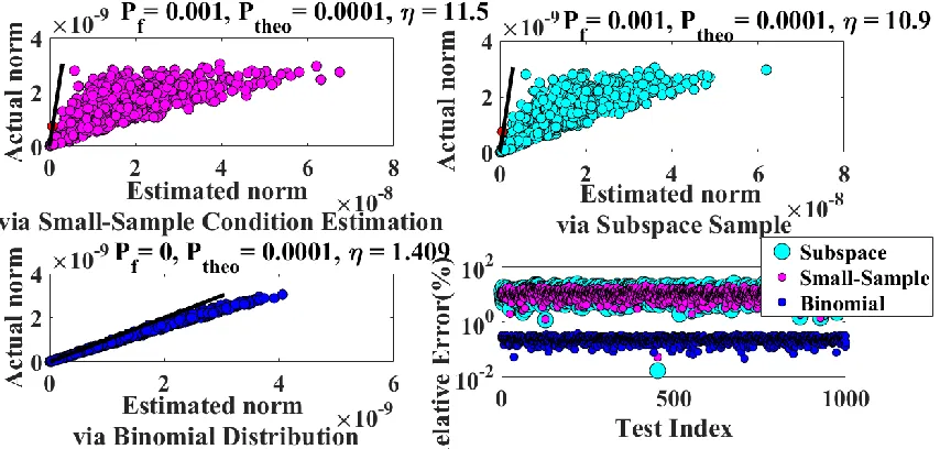
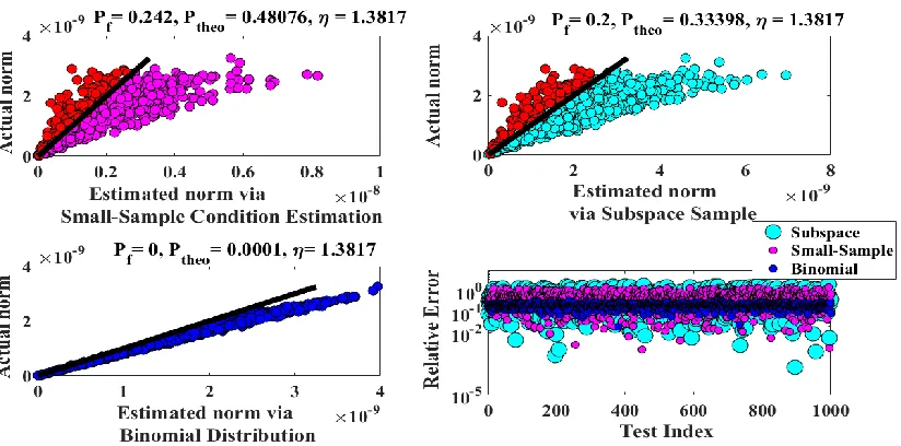
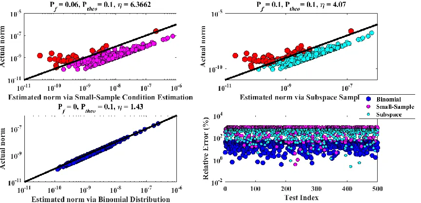
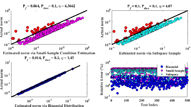
4.3.4 Proposed Binomial Estimator ...65

4.4 Propagating Error Bounds across Different Interfaces ...69

4.5 Numerical Experiments and Results ...71

4.5.1 Case Study 1: Comparison between Small-Sample Estimation and Binomial Estimator ...72

4.5.2 Case Study 2: Bounding a Nonlinear Vector-Valued Function ...79

4.5.3 Case Study 3: Propagation of Error Bounds ...102

4.6 Conclusions ...118

CHAPTER 5. MULTI-LEVEL REDUCED ORDER MODELING (MLROM) ...120

5.2 MLROM Methodology ...121

5.2.1 Mathematical Description ...122

5.3 Numerical Experiments and Results ...123

(12)

5.3.2 Case Study 2: Finding the dominant fuel (UO2 or MOX) in the Active

Parameter Subspace ...130

5.3.3 Case Study 3: Finding most Informative Pin Cell(s) in a Full Assembly ...136

5.3.4 Case Study 4: Construction of the Domain of Validity of Active Subspace using MLROM ...145

5.4 Conclusions ...155

(13)

LIST OF TABLES

(14)

LIST OF FIGURES

1-1 ROM Methods ...2

2-1 Core Calculation Levels ...18

2-2 Computational Sequence ...19

2-3 Cross Sections Discretization Over Energy ...22

3-1 Active Parameter Subspace Identification ...39

3-2 Active Response Subspace Identification ...42

3-3 Active Parameter and Response Subspaces Identification ...42

4-1 Uniform Distribution ...64

4-2 Normal Distribution ...64

4-3 Binomial Distribution ...65

4-4 Multiplier Values vs. N ...67

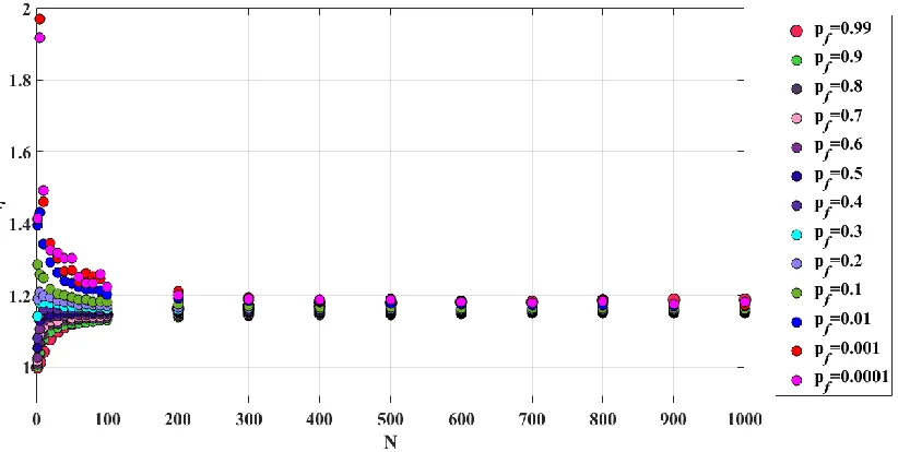
4-5 Binomial Multiplier vs. N for different probabilities of failures ...68

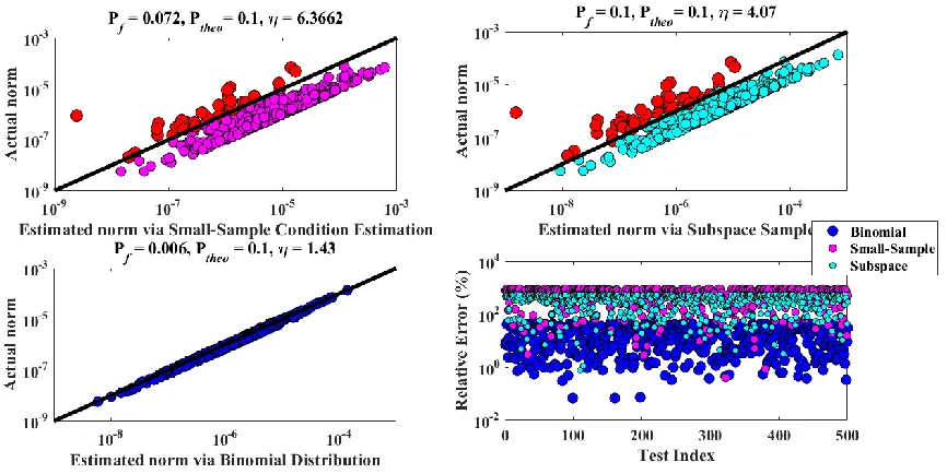
4-6 Comparison between norm estimation methods (Pf = 0.1, s = 1) ...73

4-9 Comparison between norm estimation methods ( 5 , s = 1) ...77

4-10 Comparison between norm estimation methods ( 1.241 , s = 1) ...78

4-11 Comparison between norm estimation methods (1.3817 , s = 4) ...79

4-12 Comparison of Errors in y₁ ...81

4-13 Comparison of Errors in y2 ...81

(15)

4-16 Comparison of Errors in y₅ ...83

4-17 Comparison of Errors in y₆ ...83

4-19 Comparison of Errors in y₈ ...84

4-20 Comparison of Errors in y₉ ...85

4-21 Comparison of Errors in y₁₀ ...85

4-23 Comparison of Errors in y₁₂ ...86

4-24 Comparison of Errors in y₁₃ ...87

4-25 Bounds of y1at different runs. ...88

4-26 Bounds of y₂at different runs. ...88

4-27 Bounds of y₃at different runs. ...89

4-29 Bounds of y₅at different runs. ...90

4-30 Bounds of y₆at different runs. ...90

4-31 Bounds of y₇at different runs. ...91

4-33 Bounds of y₉at different runs. ...92

(16)

4-36 Bounds of y₁₂at different runs. ...93

4-37 Bounds of y₁₃at different runs. ...94

4-38 Errors in y1due to Projection onto all subspaces. ...95

4-39 Errors in y₂ due to Projection onto all subspaces. ...95

4-40 Errors in y₃ due to Projection onto all subspaces. ...96

4-41 Errors in y₄ due to Projection onto all subspaces. ...96

4-42 Errors in y5 due to Projection onto all subspaces. ...97

4-43 Errors in y₆ due to Projection onto all subspaces. ...97

4-44 Errors in y₇ due to Projection onto all subspaces. ...98

4-46 Errors in y₉ due to Projection onto all subspaces. ...99

4-47 Errors in y₁₀ due to Projection onto all subspaces. ...99

4-49 Errors in y₁₂ due to Projection onto all subspaces. ...100

4-50 Errors in y₁₃ due to Projection onto all subspaces. ...101

4-51 Active subspaces from individual responses and from the pseudo response...102

4-52 Thermal collision rates errors - parameter reduction only (3GWd/MTU, Hot). ...104

4-53 Fast collision rates errors - parameter reduction only (3GWd/MTU, Hot). ...104

4-54 Thermal collision rates errors - response reduction only (3GWd/MTU, Hot). ...105

(17)

4-56 Thermal collision rates errors - both reductions (3GWd/MTU, Hot). ...106

4-57 Fast collision rates errors - both reductions (3GWd/MTU, Hot). ...107

4-58 Thermal collision rates errors - parameter reduction only (24GWd/MTU, Cold). ...108

4-59 Fast collision rates errors - parameter reduction only (24GWd/MTU, Cold)...108

4-60 Thermal collision rates errors - response reduction only (24GWd/MTU, Cold). ...109

4-61 Fast collision rates errors - response reduction only (24GWd/MTU, Cold)...110

4-62 Thermal collision rates errors - both reductions (24GWd/MTU, Cold). ...110

4-63 Fast collision rates errors - both reductions (24GWd/MTU, Cold). ...111

5-1 2x2 Mini PWR assembly. ...125

5-2 Maximum and Mean Error Bounds for UO2 flux (LF Model). ...126

5-3 Maximum and Mean Error Bounds for MOX flux (LF Model). ...127

5-4 Errors in UO2 Fast Flux (HF Model). ...128

5-5 Errors in UO2 Thermal Flux (HF Model). ...128

5-6 Errors in MOX Fast Flux (HF Model). ...129

5-7 Errors in MOX Thermal Flux (HF Model). ...129

5-8 15 Pins row of a PWR assembly (HF Model)...131

5-9 UO2 pin cell with large reflector region (LF Model). ...131

5-10 Maximum and mean error bounds in the material flux of UO2 from the (LF Model). ....132

5-11 Errors in fast UO2 material flux (HF Model). ...133

5-12 Errors in thermal UO2 material flux (HF Model). ...134

5-13 Errors in fast MOX material flux (HF Model)...135

5-14 Errors in thermal MOX material flux (HF Model). ...135

(18)

5-16 Fuel Pellet, Fuel Rod, and Fuel Assembly. ...138

5-17 Fast Flux Error (15 GWd/MTU). ...140

5-18 Thermal Flux Error (15 GWd/MTU). ...141

5-25 Scatter Visualization for the 9 pin cells’ Active Subspaces. ...146

5-26 Fast Flux Error (2.93% UO2 Pin Cell, 3% gd.). ...148

5-27 Thermal Flux Error (2.93% UO2 Pin Cell, 3% gd.). ...148

5-28 Mixture 500, LF. ...149

5-29 Mixture 4, LF. ...149

5-30 Mixture 1 (30 GWd/MTU, Hot Conditions). ...150

5-36 Mixture 203 (20 GWd/MTU, Cold Conditions). ...153

5-37 Mixture 212 (20 GWd/MTU, Cold Conditions). ...154

(19)

CHAPTER 1

INTRODUCTION

To understand the behavior of real-world complex systems, one must be able to model in detail the various phenomena affecting the system’s macroscopic behavior. For systems that are sufficiently complex like nuclear reactors, the associated models can be extremely expensive which may render their use computationally impractical for routine engineering calculations. To overcome this challenge, some level of reduction is typically required to allow repeated execution for routine engineering calculations and engineering-oriented studies such as design optimization, sensitivity analysis, and uncertainty quantification. The computational framework employed to introduce the reduction is typically referred to as reduced order modeling (ROM). ROM entails any process by which the complexity of the calculations can be reduced. The complexity can be measured in terms of the computational cost required to execute the model, the dimensionality of the state variables, and the input and output data interfaces.

1.1 Overview

In the next few subsections, we provide a short overview of different ROM methods. Our goal is to highlight the salient features of each method and its associated challenges. This is to motivate the two primary objectives of this thesis, outlined below and will be referenced later in the discussion.

(20)

 Further development of existing ROM methods to allow for a more efficient rendition of the reduced model when the original model is too expensive to execute as required by existing ROM methods.

1.2 Literature Review

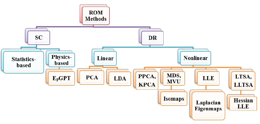
ROM methods may be classified into two categories: Surrogate Construction methods (SC) (also referred as function approximation) and Dimensionality Reduction methods (DR), as highlighted in Fig. 1-1.

To help motivate the pros and cons of ROM methods, we employ a generic model to describe the original model for which a reduction is sought. Consider a model with y responses, and x input parameters, where f is a general smooth nonlinear function, i.e., y f x

 

.

(21)

1.2.1 Surrogate Model Construction (SC)

Surrogate construction (SC) or function approximation methods aim to use an approximate representation f (also known as meta-model) as a substitute for the original function f to approximate the relationship between the input data (parameters) and the responses of interest via analytic functions with undetermined coefficients or features. This can be mathematically described as:

 



 



f x  f x (1.1)

where x n is the original feature, while

 

x is a linear or a nonlinear map that maps

x to a different n-dimensional space via transformations that preserve either local or global properties depending on the algorithm used, but gets rid of the correlation between the original variables. These algorithms aim to reduce dimensionality, reduce complexity and try to reveal the so-called latent variables necessary to describe the system after de-correlating the original n

variables. In nuclear applications x can be the cross sections which are known to have noticeably high degree of correlation resulting from constraints dictated by either the physics or the designer herself.

(22)

1.2.1.1 Statistics-based Surrogate Construction

In this category, the surrogate functional form is heuristically selected, relying either on the modeler’s experience gleaned from a large number of model executions conducted over a wide range of operational conditions or dictated by techniques such as Guassian Processes. Analysis of these executions provides observable trends that enable the modeler to identify a palette of mathematical functions that she believes are representative of the model behavior over the range of conditions of interest to the application.

A wide variety of methods falls under this category such as linear regression, polynomial chaos expansion, stochastic collocation, Lagrange polynomial expansion, polynomial response surface (PRS), radial basis function (RBF), radial basis neural network (RBNN), kriging (KRG), support vector machines (SVMs), etc.[1, 2].

(23)

build a response surface of a Rosenbrock function. Chen et al. (2006) [8] developed a surrogate using tensor product basis functions to perform sensitivity analysis and uncertainty quantification to optimize the design of an engine piston. Liem (2007) [9] developed a multi-agent collective method on an aviation system for environmental impact by estimating aircraft emissions. Bliznyuk et al. (2008) [10] hybridized RBF and Gaussian Processes interpolants with Markov Chain Monte Carlo. Of course the RBF and the GPs interpolants aimed to reduce the computational cost and hence lend feasibility to the MCMC integrals.

(24)

Finally, Yankov (2015) presented a full analysis of reactor simulations using non-intrusive techniques to build the surrogate models such as kriging and anchored-ANOVA decomposition [19] coupled with collocation techniques.

Polynomial Chaos techniques were born from the stochastic finite elements and had been conducted in nuclear applications, aiming to expand variables from the governing partial differential equations in terms of orthogonal polynomials usually followed by some sort of orthogonal projection such as Galerkin projections. Nuclear engineers often look at this from the same perspective as expanding scattering cross sections in terms of Legendre polynomials. Similar to other spectral methods, this enables the collocation of Uncertainty Quantification (UQ) under the generality of stochastic sampling but still inherit the accelerated convergence of the deterministic methods. In (2007) Williams [20] used polynomial chaos to trace how random material properties can affect radiation transport through a slab. In (2011) Fichtl and Prinja [21] employed polynomial chaos-collocation to draw a picture of how the uncertainties in total cross sections reflect in the scalar flux probability density function in both absorbing and diffusive media. Nonlinear polynomial chaos was conducted by Ayres and Williams (2013) [22] to relate uncertainties in cross sections to uncertainties in eigenvalue, they leveraged the use of linear methods against the non-linear conventional polynomial chaos by performing some sort of simultaneous diagonalization of matrices which yielded accurate results yet faster than the nonlinear PC with a factor that sometimes reaches more than 100.

(25)

wider range of operational conditions. This is because many of these surrogate model forms are selected statistically, i.e., not informed by the physics of the simulation. This limits the use of surrogate models constructed in this fashion to be used for interpolation purposes only, typically done at points in the parameter space which are close to the training points used to determine the unknown coefficients/features of the surrogate model. The second challenge facing SC methods is that the number of model executions required for training can be overwhelmingly high for complex models such as those encountered in reactor analysis problems. This is because the number of required model executions is a function of the number of parameters as well as the order of the nonlinearity of the model, that is to say, if the modeler is building a linear surrogate for a model with n parameters then, at a minimum n executions of the original model are required. This could be prohibitive in reactor physics where the number of parameters could be in the order of 106_{. For higher order models, e.g., 2}nd_{order, the number of model executions} typically grow exponentially, which is often referred to as the curse of dimensionality.

1.2.1.2 Physics-based Surrogate Construction

(26)

et. al., 2013 [23], where he combined reduced basis methods, range finding algorithms with generalized perturbation theory to construct a unified framework that enables the reduction of high overhead computations involved in reactor calculations with errors that are within the machine precision and hence came the terminology Exact-to-precision generalized perturbation theorem (EPGPT). Another example would be the work of Mickus et al. (2014) [24] work which proposed an approach to physics-based surrogate for application with Integrated Deterministic Probabilistic Safety Assessment. In this method, the authors chose not to use the well-known Neural Networks methods since there is no actual physics modeling rendered, in addition to the huge number of data points required for the fitting process. This leads to some lack of reliability and robustness of the surrogate model outside the experimental domain given that any extrapolation will acquire no physics reasoning. Instead, the authors selected the most important physical phenomena to be resolved by the surrogate model and then calibrated the model to capture parameters that were not directly modeled in the surrogate and hence arrived at an intermediate stage between pure neural networks and analytical solutions.

1.2.2 Dimensionality Reduction (DR)

(27)

 



 



f x  f x (1.2)

where n

x is the original n-dimensional feature and

 

x is again either a linear (LDR) or a nonlinear map (NDR) that maps the original feature to a world of non-correlated variables.

If the relationship between the reduced variables and original variables is linear, the reduced variables are described by subspaces, denoted hereinafter by “active subspaces”, and the reduction methods are referred to as linear DR or LDR for short. The use of subspaces provides two advantages, a geometric advantage which allows one to provide an intuitive understanding of the mechanics of reduction, and a mathematical advantage wherein linear algebra and matrix theory methods may be leveraged to describe the reduction [25-28].

In LDR, all variables variations that are orthogonal to the active subspaces are considered to have a negligible impact on the model behavior as measured in terms of its key responses of interest. This implies that the physics model as applied to the engineering application of interest constraints the variables variations to the active subspace, and/or that variables variations that are orthogonal to the active subspace have very low sensitivities for the responses of interest.

The implication of LDR is that one can recast many engineering analyses whose cost directly depends on the number of input parameters and/or output responses into a reduced form that is described by the reduced variables.

(28)

in the order of 104-109 whereas the number of reduced variables is in the order of 102 variables only. This dramatic reduction can enable these analyses to be computationally tractable.

For LDR methods to be reliable, one must be able to characterize the errors resulting from constraining the variables variations to the active subspaces only. This represents one of the objectives of this thesis where the aim is to develop upper-bounds on the LDR errors when the reduction is rendered at some or all of the models interfaces, including the parameters and the responses for single and multi-physics models.

(29)

Another important extension of the basic LDR idea is the work by Fisher on Linear Discriminant Analysis (LDA) in 1936 for classification [31]. LDA expands the dependent variables as a linear combination of measured features by searching for a linear map to maximize some measure of separability between data points to allow for credible classification.

Before ending this section, we note that DR may be rendered in a nonlinear manner as well, meaning that the relationship between the original and reduced variables may be selected to be nonlinear, implying nonlinear dimensionality reduction or NDR for short. NDR methods are categorized into three families depending on what the method preserves while searching for the required map (i.e., the linear or nonlinear transformation of the original and the reduced variables): methods that preserve local properties such as Local Linear Embedding (LLE) [32], Laplacian Eigen Maps [33], and Hessian Local Linear Embedding (HLLE) [34], methods that preserve global properties such as Multidimensional Scaling (MDS) [35], Isomaps [36], Kernel PCA [37], diffusion maps [38], Generalized Discriminant analysis (GDA) [39, 40], Multilayer Autoencoder [41], Stochastic Neighbor Embedding (SNE) [42]. Or methods that perform global alignment of local properties like Locally Linear Coordination (LLC) [43].

(30)

And finally, because NDR usually succeeds on tailored highly nonlinear problems such as the well-known Swiss roll dataset, while the real applications success for NDR is scarce, especially that a vast number of NDR techniques flourish with complex topologies, high curvatures, clustered, noisy, or sparse data, which is not the case in nuclear applications [48].

1.2.2.1 Mathematical Representation of LDR Methods

A nonlinear function f with n input parameters and m output responses is said to be reducible and of parameters intrinsic dimension r_x(0 r_x n) and response intrinsic dimension

(0 )

y y

r  r m if there exists an nn operator

P

xwith a rank of rx and an mm operator

y

P with a rank of r_ysuch that r_x and r_y are the smallest integers satisfying:

 

y x .

f x f x

x S

f x 



  

P P

(31)

In our context, P_xand P_yare projector operators onto the parameter space and response

space respectively, such that T

x  x x

P U U and T

y  y y

P U U where n rx

x





U and m ry

y





U are

matrices containing the orthonormal columns spanning the active parameter and response subspaces respectively. The intrinsic dimensionalities of these operators, i.e.

 





dim R P_z r_z; zx y, - with R being the range of the operator Pz - are typically much

smaller than the original dimensions of the parameters and responses spaces, i.e.

max( , )r r_x _y min( , n)m . The algorithms to construct these matrices are discussed in details in Chapter 3. Further, we show that this inequality condition may be satisfied in a probabilistic sense with a high probability of 1-10-s, where s is a small integer representing an additional number of model executions, referred to as over-samples, more details about this will be presented in Chapter 4.

We make several remarks about this LDR definition. First, note that the definition makes no assumptions about the properties of the function f, implying that while the relationship between the reduced and original variables is linear, as given by the above equation, the function

f being reduced can, in general, be nonlinear.

(32)

models, the original model dimensions are in the order of millions, whereas the reduced model dimension is sought to be in the order of few hundred variables only. With limited model evaluations of the order of the reduced dimension r,

Third, if the inequality condition can indeed be satisfied with small r and acceptable tolerance, the implication is that a limited number of degrees of freedom r in the active space is sufficient to characterize to a high level of accuracy all possible response variations, whose original dimensionalities are often much larger than r. Mathematically, this means that parameter perturbations belonging to the active parameter subspace are the ones responsible for the observed model response variations, whereas all parameter perturbations that are orthogonal to the active subspace induce negligible variations in the responses, which can be bounded by the tolerance.

Finally, to gain computational efficiency in subsequent engineering analyses requiring multiple model executions, ROM confines all parameter perturbations to the active subspace, since its dimensionality is much smaller than the original parameter space. For example, one can recast all engineering analyses, such as UQ and SA, in terms of the reduced variables

 r T rx

x

x U x , premised on the assumption that they describe all important parameters variations.

(33)

cross-sections used in downstream core calculations as functions of a wide range of conditions, such as the assembly type, fuel burnup, fuel and coolant temperature, poison content, etc. This requires several thousands of flux evaluations which could be rendered more efficiently using ROM methods.

(34)

CHAPTER TWO

NUCLEAR REACTOR CALCULATIONS

2.1 Design Calculations

Nuclear reactor physics calculations, representing the focus of our work, are overviewed in this chapter. Reactor physics calculations model the transport of neutrons inside the reactor core and the change in fuel isotopics and other core materials due to radioactive transmutation over the expected range of reactor operational conditions. The fundamental equations employed are the Boltzmann equation which describes the transport of neutrons and the Bateman equation which describes the transmutation of fuel and other core materials isotopics. The salient features of these equations are described here to set the stage for the discussion of ROM methods.

The primary source of heat in fission reactors is due to the scission of heavy nuclei by slow (i.e., thermal) or energetic (i.e., fast) neutrons. Shortly after the scission of a nucleus, two lighter nuclei, called fission fragments, few neutrons, called prompt neutrons, and few gamma rays, called prompt gamma, are released. The majority of the mass defect, the difference between the mass of the original heavy nucleus and the combined mass of lighter fission fragments and prompt neutrons, is released in the form of kinetic energy imparted to the fission fragments and prompt neutrons. One typical fission reaction is described by the following equation:

235 140 94

92 54 38 2 200

n U  Xe Sr n MeV

(35)

primarily by the newly born neutrons. The goal of reactor core design is to ensure that the number of neutrons born in a given generation is equal to the number born in the previous generation to ensure the reaction is sustainable and controllable. When this balance is established, the reactor is said to be critical, with the criticality described using the multiplication factor k which measures the ratio of neutrons production to neutron loss by parasitic absorption and leakage. Parasitic absorption implies a neutron capture event that does not lead to fission, e.g., the capture of neutron under the low-lying resonances of U-238, captured by special materials, called neutron absorbers, deliberately introduced into the reactor to control criticality. The goal is to keep k at a value of 1.0 throughout operation by continually balancing neutron loss and production terms. When k < 1.0 or k > 1.0, the number of neutrons will decrease or increase forming subcritical or supercritical reactors, respectively. When the reactor power is to be increased, k is increased for a short period of time by reducing neutron loss until the desired power level is reached, then k is returned back to a value of 1.0.

(36)

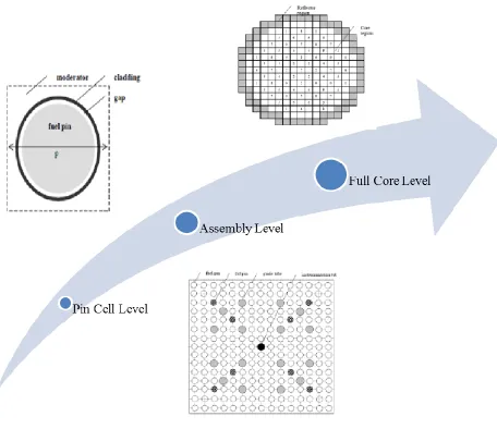
Fig. 2-1. Core Calculation Levels.

(37)

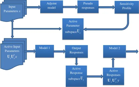
Cross-sections are the basic nuclear parameters that characterize the probability of interaction between neutrons and various core materials. Given the complicated dependence of cross-sections and the heterogeneous core design, the neutron flux becomes a complicated function of space, energy, angle, and time. The first two level focus in detail on the energy, and angle dependence of the neutron flux, whereas the third level describes in details the spatial and temporal dependence. This separation of dependencies has proven to be an effective approach for reactor physics calculations. Before explaining these levels, we introduce the neutron transport equation to highlight some of the challenges associated with its solution for reactor problems. Figure. 2-2 depicts the flow diagram for the calculation procedure.

Fig. 2-2. Computational Sequence.

(38)

2.1.1 Neutron Transport Equation (Boltzmann Transport Equation)

The equation governing the neutrons distribution in a reactor core is referred as the Neutron Transport Equation (also known as the Boltzmann Equation) can be written in various forms due to the assumptions and simplifications that can be carried out to render the equation suitable for the required application and analytically solvable if possible. In most forms the dependent variable is the angular neutron flux in [#/cm2 /sterad/ MeV/sec]









t



 







Leakage rate density Total Collision rate External source generation rate rate of change

0

1 _ˆ _ˆ _ˆ _ˆ _ˆ _ˆ

, , , , , , Σ r,Ω,E,t ψ r,Ω,E,t , , ,

ˆ ˆ

, ,

ext

s

r E t r E t S r E t

v t dE r     _ _{  } _ _ _ _    

_





  

 



 

_

_

_

_

4 scattering Rate 0 4 Fission rate ˆ ˆ , , , , ˆ ˆ , , , , , 4 f

E E t r E t d

E

dE r E t r E t d

                    



 

(2.1)

where  is the angular neutron flux [neutrons cm-2 sec-1 sterad-1 MeV-1], and _f are the macroscopic total and fission cross sections, respectively in [cm-1]; v is the average neutrons speed in [cm sec-1];  is the average number of neutrons produced per fission reaction. The

angular variable ˆ v

v

  is a unit vector in the direction of the neutron travel and r is the

position vector of the neutron.  is the fission spectrum and finally _s is the double differential macroscopic scattering cross section in energy and direction.

(39)

another equation, that describes the change in various materials concentrations, assumed to be input to the Boltzmann equation. For example, the macroscopic cross sections depend on the number densities, i.e., isotopic concentrations. Number densities are calculated using the Bateman equation which is a system of ordinary differential equations that are used to update the nuclei concentrations based on their respective production and loss terms. The production and loss terms depend on the neutron flux which is calculated by the Boltzmann equation. To decouple the Boltzmann and Bateman equation, the quasi-static assumption is typically used, where the reactor core is assumed to operate at steady state for a short period of time during which the number densities are assumed constant to solve for the flux; then the flux is used to calculate the production and loss rates for the various nuclei which are used to update the nuclei via the Bateman equation.

Given the steady-state assumption, the Boltzmann equation is assumed to have a solution, which is only possible if the reactor is critical. To overcome this, the k-eigenvalue is introduced as a knob that determines the deviation from criticality. The designers can change the various model features to ensure k is as close to 1.0 as possible throughout the core life. Eq. (2.1) can then be written as:







 





 



 

_

_

_

_

t 0 4 0 4 ˆ ˆ

ˆ _{, ,}ˆ _{Σ r,Ω,E ψ r,Ω,E} _, ˆ ˆ_, _{, ,}ˆ ˆ

1 _ˆ _ˆ

, , , 4

s

f

r E dE r E E r E d

E

dE r E r E d

k                                     

 

(2.2)

here the k-eigenvalue is the multiplication factor.

(40)

render numerical solutions, the energy range is split over multiple ranges, where the cross-section is assumed constant over each range. These ranges are called neutron groups, and the corresponding constant values are referred to as group cross-sections. In the group representation, the Boltzmann equation may be re-written as:

 

   



  

 

t,g , 1 4 , 0 4 ˆ ˆ

ˆ _, ˆ _Σ _{r,Ω ψ} _r,Ω _,ˆ ˆ _, ˆ ˆ

1 _ˆ _ˆ

, 4

Ng

g g s g g g

g

g f g g

r r r d

dE r r d

k                                   

 

 

(2.3)

This equation is achieved by integrating eq. (2.2) w.r.t to energy over the gth_{energy group (i.e.,}

1 g g E E dE  



) where Ng is the total number of groups in the selected energy structure which is

dictated by the required accuracy. The figure below shows the continuous cross-section and the group cross-sections which are piecewise constants. The primary challenge of reactor physics calculations is the ability to calculate the group cross-sections in a manner that preserves the reaction rates and the multiplication factor.

(41)

2.1.2 Multi-group Cross-section Generation

In this step, the pointwise cross-sections are collapsed into a multi-group structure using assumed flux shapes. This structure is decided based on an educated trial and error relying on expert judgment attempting to resolve all aspects of the flux spectrum, expected to affect the integral quantities of interest such as eigenvalue, reaction rates, etc.

The uncertainties of the multi-group cross-sections can be estimated by propagating the uncertainties of the nuclear reaction model parameters using the standard sandwich relationship. The multi-group cross-sections contain essentially two different sources of uncertainties, one originating from the nuclear reaction parameters used to construct the continuous cross-sections, and the other from the assumed flux shape. Most tools account only for the first source of uncertainty (assuming linearity). Whereas the flux shape uncertainty is difficult to estimate because the real flux shape is unknown a priori. Therefore, assumed flux shape uncertainty must be treated as a source of modeling uncertainty. To estimate this source, one must be able to compare the predictions against a high fidelity model that directly uses the continuous cross-sections, i.e., without any collapsing. The discrepancies between the predictions of the low and high fidelity models can be used estimate the modeling bias, which has to be repeated to take into account its dependence on other modeling conditions, such as composition, temperature, etc., i.e., control parameters. The group averaged cross sections are computed as follows:

 





4

ˆ ˆ

, ,

E r E d



 



   (2.4)

 

1



,



g

E g

E

r E r dE

 



(42)



 



   

1 , , , g g E

x x g g

E

E r  E r dE r  r



  



(2.6)

  







1 1 , , , g g g g E x E

x g E

E

E E r dE E r dE

      



(2.7)

where x can be total, fission or absorption reaction.

  

 





 



1 1 , , , , g g g g E f E g E f E

v E r E r E dE

r E r E dE

       



(2.8)

  







1 1 1 , 1 , g g g g E E g E E

r E dE v E

v

r E dE

    



(2.9)



 







1 1 1 , , , , g g g g g g E E s E E

s g g E

E

dE dE r E E r E

r E dE

              



(2.10)

2.1.3 Lattice Cell Calculation

(43)

the entire lattice. The few-group cross-sections are subsequently used in core-wide calculations which are 3D models of the entire reactor core. The goal here is to model each assembly as a group of axial nodes, where each node is represented in core-wide calculations as a uniform region with few-group cross-sections. This requires the ability to smear all the energy and spatial dependence of the cross-sections at the lattice level prior to entering core-wide calculations. This smearing process is referred to as homogenization and is carried out as follows.

In this step, one calculates the few-group cross-sections for the cell lattices. These

calculations must be repeated every time a new cell lattice design is introduced. Cell lattice

calculations start with the multi-group cross-sections and calculate the few-group cross-sections

for a wide range of core conditions.

To provide an idea of the size of the data streams flowing through cell lattice

calculations, consider a typical transport code that is used to calculate the few-group

cross-sections. The code is to be executed a number of times equal to NB x NC x NL times,

where NB refers to the number of burnup steps, and NC is the number of branch cases required to

functionalize cross-section dependence on core conditions such as fuel and coolant temperature,

coolant voiding, boron content, etc., and NL is the number of cell lattice types in the core. To

propagate uncertainties, one would need to repeat these model executions N times, which is in

the order of few to several hundred. This results in in the order of 105 model executions which is

prohibitive in practical applications.

Further, if one is interested in identifying the dominant contributors to the propagated

uncertainties via an SA, one needs to execute the solver a number of times that is proportional to

(44)

cross-sections. This increases the number of required code runs to be in the order of 106 to 109

executions, which is overwhelmingly high despite the expected increase in computer power.

In this step, two sources of uncertainties are introduced, one from the multi-group cross-sections

propagated from the previous step, and the other resulting from the modeling assumptions, such

as the use of reflective boundary conditions, the use of a deterministic transport solver, and the

use of multi-group instead of continuous cross-sections. The first source is again straightforward

to account for. The computational cost becomes impractical when sensitivity information is

required, i.e., to understand the contribution of the individual multi-group cross-sections on the

propagated few-group uncertainties.

The second source depends on the modeling decisions taken and therefore must be

treated as a source of modeling errors. First, regarding the use of deterministic transport solver

and multi-group cross-sections, this source could be identified by comparing model predictions

against a high fidelity continuous cross-section Monte Carlo model. The second source is more

difficult to account for because it depends on the type of neighboring bundles in the reactor core.

Finally, similar to the previous step, the correlations between the multi-group

uncertainties and the modeling uncertainties (resulting from the transport model, multi-group

cross-sections, and neighbors’ approximations) are to be investigated.

This step can be accomplished through two sub-steps: Homogenization and Few-group Cross-section generation.

(45)

, ,

g j j g j j

j j h g h j j V V V V    







(2.11)

Then cross sections can be computed such that:

, , , ,

h h h

x g j g j j x g g j V V     



And hence: , , , , , , , , j

x g j g j j x g j g j j

j j

h

x g h h

g j g j V V V V        







(2.12)

Similar trend can be applied to the number densities:

; 1, 2,

i j j j h

i h nuclides

N V

N j N

V





 (2.13)

2.1.3.2 Few-Group Cross-section Generation. The homogenized values can then be used to prepare for the core calculations by collapsing the energies into a coarser structure. This will render the core calculations feasible with an acceptable error. This can be achieved using a similar procedure based on the conservation of reaction rates as follows:

; 1, 2,

i i h h G g g G i NG   





 (2.14)

, ,

i i

h h

x g g g G h

x G h

 





 



(46)

where NG<<Ng. This can be used in core calculation to speed it out in addition to some acceleration algorithms such as the coarse mesh finite difference acceleration (CMFD) that will not be in the scope of this report.

2.1.4 Downstream Core-wide Calculations

The last stage involves the calculation of core-wide power distribution during steady state and

transient conditions starting with the few-group cross-section data. The number of few-group

cross-sections is equal to NFG x NB x NC x NL where NFGis the number of few-group

cross-sections generated per a single transport model execution, which is in the order of 10,

representing the thermal and fast absorption sections, transport section, fission

cross-sections, prompt neutron yield, and energy release, and Xe and Sm fast and thermal absorption

cross-sections. If macroscopic depletion model for core calculations is used, the total number of

few-group cross-sections is in the order of 104. If microscopic depletion models are used, this

number is scaled by the number of nuclides tracked at the core level to account for the individual

nuclides’ cross-sections.

The sources of uncertainties in core-wide calculations include, uncertainties from the

few-group cross-sections; uncertainties from the radiation transport model employed (e.g., nodal

diffusion theory assumptions, and two energy-group cross-section representation); and

uncertainties from non-neutronic models, e.g., thermal-hydraulics models, and their associated

correlations used to describe the transfer of the heat from the fuel to the coolant, and the

corresponding feedback into neutronics calculations, e.g., fuel temperature feedback, coolant and

(47)

parameters such as the lattice dimensions, fuel composition, flow rates, inlet coolant

temperatures, etc.

The first source, i.e., few-group cross-section uncertainties, can be treated using a

standard UQ. The second source, i.e., the radiation transport model, can be estimated using the

UQ methodology via core-wide Monte Carlo models.

(48)

CHAPTER THREE

REDUCED ORDER MODELING

3.1 Introduction

(49)

3.2 Literature Review

As discussed in the introductory chapter, linear dimensionality reduction techniques have been employed by analysts to reduce the dimensionality of multi-dimensional data for over a century. In the past 15 years, interest in these techniques has been revived to support the surge witnessed in the area of predictive modeling, where high fidelity models utilizing the cheap and abundant computer power are sought to provide a better understanding of complex systems behavior such as nuclear reactors. In 2004, Abdel-Khalik [52] presented the idea of LDR under the name of efficient subspace methods (ESM), where the subspaces represent lower dimensional manifolds onto which the model variables are projected. Later, the terminology of ‘active subspaces’ was adopted by other researchers such as Russi in 2010 [54], Constantine in 2012 [56], and Webster in 2012 [57], and Abdel-Khalik in 2010 [58, 59], emulating the language of active constraints from optimization theory. The notion of active implies that variables variations along the subspaces impact the model behavior, whereas variations over the orthogonal complements, i.e., the “inactive”, as called by Abdel-Khalik in 2010, or “passive”, as called by Webster in 2012, subspaces, have negligible impact on the model behavior as measured in terms of a number of user-selected quantities of interest.

(50)

called ‘subspace methods of pattern recognition’ where he included rigorous mathematics along with interesting engineering applications for subspace methods.

Notice that in principle one can find an infinite number of active subspaces that meet a user-defined present tolerance, which bounds the discrepancies between the original functions predictions and the reduced function predictions. The goal is to find a subspace that is not necessarily unique, with a very small size rx to capture the dominant parameter variations. In our work, we show that one can find an active subspace with slightly larger size in a computationally efficient manner that outperforms existing algorithms attempting to find the smallest possible active subspace. This is possible using our proposed multi-level ROM strategy which employs approximate models, i.e., models of lower fidelity, or models constrained to sub-domains of the overall problem domain, to obtain an approximation for the active subspace.

(51)

3.3 Reduction Algorithms

This section is dedicated to providing a comprehensive overview of the theories and algorithms that form the basis for our rendition of reduced order modeling to general nonlinear models. In particular, the next 3 subsections will cover the following three subjects: identifying the active input subspace for a scalar valued function, identifying the active input subspace for a vector-valued function, and finally identifying the active response subspace algorithm [73].

3.3.1 Active Input Subspace Identification Algorithm (AISIA) for a scalar-valued function:

Let

f

:

n



be a scalar-valued nonlinear function that maps an n-dimensional input

vector of model parameters such as cross section into a single response such as the effective

multiplication factor keff. The goal is to determine the important directions in the parameter

space, i.e., directions along which a perturbation in the model parameters will cause a noticeable

impact on the response of interest. Notice that if the model is linear, there is only one such

direction, that’s the gradient of f with respect to the model parameters. For general nonlinear

models, however, there could be as many as n directions that affect the response. The goal of the

reduction is to identify rx directions that capture the response variations to a given preset

tolerance . Ideally, rx should be much less than n, the nominal dimension of the input

parameter space. The subspace forming the span of the rx directions is referred to as the active

subspace

 

_, _,

1

: rx ; n

act span ux i _i_ ux i , meaning that the original feature x can be written as the

(52)

       

variable variable

r T

r n r x r r T n r n r T

T

x x x x _{n r T} x x x x

x active inactive

x x_   _ x x    x

 _ _ U

U U U U U U U U

U

where  r n rx

x





U

is the matrix whose orthonormal columns span the active subspace, or in other

words: The active subspace is the range of U _xr , act 

 

U xr . The superscript indicates that

the new attribute  r  r x

x U x is a reduced input vector due to a linear projection of the original

feature x onto the active subspace. The matrix

U

 _xr contains rx columns which span the active

input subspace.

One may visualize this considering a two-dimensional function f that is intrinsically

one-dimensional (i.e., i1D) [74] such that:

 





1 2





 

1

T T

f x  f x x g u x ;

Then the Fourier transform of such a function will be:

 

  

1



2 1 1



T T

F w G u w  I u u w

where F, G are the Fourier transforms of f and g respectively. As follows:





 

 1 1 2 2

_

_

2

2 ₂

1 2 1 2 1 2

{ , } ,

T

i w x _i _{w x} _{w x}

f x x F w e  f x dx e  f x x dx dx

 

  

 

 





 

 

2  

_{ }

{g x } G w e i  wx g x dx;

 



(53)

and xu x₁T , wu w₁T are the reduced variables in both the original and the frequency domains. With  being the Dirac-delta function, the Fourier transform for f states that the function vanishes in the directions normal to u₁ and changes governed by the function G in the directions parallel to u₁. This can be generalized to the case where the nominal dimension is n and the

intrinsic dimensionality is r_x and f x

 

g



U _xr Tx



. In this case, the variation of the function in

the directions parallel to the subspace spanned by the r_xorthonormal columns of U _xr significant when compared to the negligible impact on f caused by an input vector that is perpendicular to that subspace. The identification of such active subspaces is accomplished using a gradient-based algorithm that constructs an active subspace in the input parameter space employing the adjoint model to calculate the first order derivatives of a general pseudo response with respect to input parameters. The pseudo-response is not a physical quantity but a mathematical abstraction representing a random linear combination of all model responses. For a justification of the use of pseudo-responses, the reader may consultsection 3.3.2.1. The algorithm may be described by the following steps:

Inputs:

x

_ref



nis the reference input vector (i.e., cross sections). x is the relative perturbation from the reference value.

f

:

n



is the forward model of interest.

f

adj

:

n



is the adjoint model (needed to compute the sensitivities).

(54)

2. Generate k random realization

 

_, _,

1; [ , ]

k _n

i i i ref i ref i

x _ x  x x x x .

3. Initialize: J[].

4. for i = 1 to k

5.

y

_i



f x

 

_i

6.

 





T

i i

j x  y

7.

J



[ ,

J

j x

 

_i

]

.

8.



U

_x

,



_x

,

V

_x





svd

 

J

.

9.







 







:,1: T :,1:

test x x test

test

f f i i

f



 X U U X

E

X .

10.



b



Construct an error bound as shown in section (4.3.4).

11. If

 

_b



_user

12.

r

_x



i

.

13. U _xr U_x



:,1:i



.

14. Return

15. end if 16. end for

(55)

3.3.2 Active Input Subspace Identification Algorithm (AISIA) for Vecor-valued functions:.

For

f

:

n



m, the above algorithm can be intuitively repeated for each component in the response vector and hence find an individual active subspace for each of the m-components as presented by Russi (2010). This renders the process impractical for large number of responses and hence motivates for the pseudo-response trick.

3.3.2.1 The Pseudo-response Trick:

Earlier work [73] has shown that vector-valued functions can be tackled using the pseudo response which is a non-physical quantity and hence find an individual active subspace for each of the m-components. This starts to be impractical right after m exceeds 10. In a typical reactor physics application, m might be in the order (104-106) which motivates the need for a way to get around this obstacle and render the algorithm feasible even for huge response vectors.

Mathematically, the pseudo response is just a random linear combination of the response components R_ipseudo w y xT

 

_i where w is the weighting vector. This can be analogous to what is done in the input perturbation process since a random input perturbation reflects a movement in random directions in the input space, in the adjoint world a similar trend is to randomly perturb the response vector which can be accomplished via a random linear combination of the response vector.

In [73] the authors showed that one can extract the active subspace using the sensitivity profile of the pseudo response w.r.t. the input parameters. The procedure goes as follows:

Inputs:

x

_ref



nis the reference input vector (i.e., cross sections).

(56)

:

n m

f



is the forward model of interest.

:

adj n m

f



is the adjoint model (needed to compute the sensitivities).

1. Set 



x x:  n;x_ref



1x



 x x_ref



1x





is an n-dimensional hyperrectangle.

2. Generate k random realization

 

_, _,

1; [ , ]

k n

i i i ref j ref j

x _ x  x x x x .

3. Initialize: J[].

4. for i = 1 to k

5.

y

_i



f x

 

_i

6.

R

_ipseudo



w y

T _i , where w are some random weights.

7.

 



pseudo



T

i i

j x  R [using the adjoint model].

8.

J



[ ,

J

j x

 

_i

]

.

9.



U

_x

,



_x

,

V

_x





svd

 

J

.

10.







 







:,1: T :,1:

test x x test

test

f f i i

f



 X U U X

E

X .

11.



b



Construct an error bound as shown in section (4.3.4).

12. If

 

_b



_user

13.

r

x



i

.

14. U _xr U_x



:,1:i



.