Modeling the transmission of vancomycin-resistant enterococcus (VRE) in hospitals: A case study

(1)

Modeling the Transmission of Vancomycin-Resistant

Enterococcus (VRE) in Hospitals: A Case Study

A. R. Ortiz1_{, H. T. Banks}2_{, C. Castillo-Chavez}1_{, G. Chowell}1_, C. Torres-Viera3 _{and X. Wang}1

1 _{School of Human Evolution and Social Change} Arizona State University

Tempe, Arizona 85287-2402

2_{Center for Research in Scientiﬁc Computation} North Carolina State University

Raleigh, North Carolina 27695-8212 3_{South Florida Infectious Diseases}

8700 Tyndall Drive, Suite 100 Miami, Fl 33176

(2)

Abstract

Nosocomial, or hospital-acquired infections, the fourth cause of death in the US, are evidence that hospitals provide not only medical care but also harbor pathogens that pose serious, often fatal, risks of infection, particularly to the young, the el-derly, and immune-compromised individuals. Infection-control measures aimed at reducing their impact are being implemented with various degrees of eﬃciency at US hospitals. Data from general and oncology hospital units on Vancomycin-resistant Enterococcus (VRE), one of the most prevalent and dangerous pathogens involved, are used to highlight the importance of modeling nosocomial infection dynamics as a prelude to the testing and evaluation of control measures.

New mathematical models of the transmission dynamics of VRE in hospitals are introduced in order to identify and quantitatively assess the time evolution of nosocomial infections. Ordinary differential equation (ODE) and discrete delay dif-ferential (DDD) models in conjunction with statistical methods are used to estimate key population-level nosocomial transmission parameters. This framework is tested using unpublished surveillance data from two types of hospital units. The popu-lation is divided into uncolonized, VRE colonized, and VRE colonized-in-isopopu-lation categories and the use of constant and variable rates of isolation admitted with VRE or VRE-colonized during hospital stays is evaluated in models including health care workers’ hand-hygiene compliance. The process of model calibration detected irreg-ularities in the available surveillance data; these irregirreg-ularities that are most likely the result of the data recording-process. Efforts to fit data within our highly flex-ible dynamic-modeling framework suggest that clinical-trial level surveillance data is needed.

(3)

1 Introduction

People go to the hospital to be treated for their health problems, believing they will be discharged in better health than when they were admitted. Hospitals and health care professionals are committed to improve the health of their patients. However, there are risks associated with the provision of health care with one of the most important being the acquisition of infections at hospitals. The Centers for Disease Control and Prevention (CDC) estimates that 5% to 10% of patients, or more than two million patients each year will get an infection while in a United States hospital with about 90,000 of them dying from such infections [19]. These hospitals-acquired infections or nosocomial infections are infections not present or incubating in a patient at the time of admission to a hospital or health care facility. If symptoms ﬁrst appear 48 hours or more after a hospital admission or within 30 days after discharge, they are considered nosocomial infections. Studies reveal that about 70% of bacteria that cause nosocomial infections are resistant to at least one antibiotic commonly used to treat them [40]. Three decades ago infection-control measures were put in place to infection-control antibiotic-resistant nosocomial infections and yet these infections have continued to increase. Multidrug-resistant pathogens have become increasingly problematic, especially in the critical care setting, according to the CDC’s National Nosocomial Infection Surveillance System (NNIS System).

Nosocomial infections have been classiﬁed as: urinary-tract infections, surgical-incision infections, pneumonia infections, blood-stream infections, skin infections, gastrointestinal-tract infections, and central-nervous-system infections. The urinary-gastrointestinal-tract infections are the most prevalent type of nosocomial infection as they account for about 35% of all nosocomial infections [40]. Studies have demonstrated that these infections occur after urinary catheterization. The surgical-incision infections account for about 20% [40] of nosocomial infections. Pneumonia infections account for about 15% of nosocomial infec-tions [40] in which the most susceptible individuals are those with chronic obstructive pulmonary disease or those utilizing mechanical ventilation. Blood-stream infections account for another 15% of nosocomial infections [40].

Nosocomial infections may cause severe morbidity in patients leading to extended hospital stays. The average number of extra days a patient has to spend in the hospital varies depending on the type of nosocomial infection: 1 to 4 extra days for urinary-tract infections; 7 to 8 extra days for surgical-incision infections; 7 to 21 extra days for blood-stream infections; and 7 to 30 extra days for pneumonia infections [18]. Further, deaths due to nosocomial infections are the fourth leading cause of death following heart disease, cancer, and stroke [1].

(4)

1.1 VRE as an antibiotic resistant pathogen

Most of the nosocomial infections are primarily caused by antibiotic resistant pathogens, such as Vancomycin-resistant Enterococcus (VRE). VRE is the group of bacterial species of the genus enterococcus that is resistant to the antibiotic vancomycin and it can be found in the digestive/gastrointestinal, urinary-tracts, surgical-incision, and blood-stream sites. The CDC during 2006 and 2007 reported that enterococci caused about 1 of every 8 infections in hospitals and about 30% of these are VRE [21].

The bacteria responsible for VRE can be a member of the normal, usually commensal bacterial flora that becomes pathogenic when they multiply in normally sterile sites. Currently there are six different types of vancomycin resistance shown by enterococcus: Van-A, Van-B, Van-C, Van-D, Van-E and Van-F. Of these, only Van-A, Van-B and Van-C have been seen in general clinical practice so far. The significance is that Van-A VRE is resistant to both vancomycin and teicoplanin antibiotics, Van-B VRE is resistant to the antibiotic vancomycin but sensitive to antibiotic teicoplanin, and Van-C is only partly resistant to the antibiotic vancomycin, and sensitive to antibiotic teicoplanin. In addition, VRE has an enhanced ability to pass resistant genes to other bacteria.

1.1.1 Colonization and transmission.

There is a distinction between VRE colonized individuals and VRE infected individuals. The former means that the organism is present in or on the body but is not causing illness while the latter means that the VRE is present and causing illness. Colonization is a VRE carrier state preceding potential infections. This distinction is important in VRE screening [17] since VRE colony counts are similar in the stools of colonized and infected patients. A hospital facility may be adequately reporting its infection rate if its VRE rate is based solely on clinical cultures of VRE infected patients, but it may be underestimating the true burden (and therefore potential transmissibility) of VRE. Screening for patients colonized by VRE provides information about potential sources of illness. The goal of screening is to identify as many VRE colonized patients as possible so that infection control measures that decrease transmission and reduce the number of VRE infected patients can be put in place.

The duration of colonization could last from weeks to months. A study has shown that patients in a university hospital had a mean length of VRE colonization of 204 days (29 weeks) ranging from 4 to 709 days [14]. The factors most associated in predisposing VRE colonization to patients includes: a compromised immune system or nutritional status, the use of catheters (such as urinary or central venous), co-morbidities (e.g., diabetes, renal insuﬃciency, cancer), length of stay in the hospital, inadequate infection control practice among health care workers (HCW), and prolonged antibiotic used (>

10 days). Hence VRE patients admitted in hospital units such as intensive care and oncology have a greater colonization risk.

(5)

direct-contact transmission or indirect-contact transmission. Direct-contact transmis-sion involves direct physical contact (mostly hands) that results in the physical transfer of microorganisms between a susceptible host and a colonized agent such as a patient who is infected or carrying the organism. Indirect-contact transmission involves contact between a susceptible host and a contaminated institutional environment, that includes health care workers (human vectors).

1.1.2 Treatment and interventions

People who are colonized with VRE do not usually need treatment. Most VRE infections can be treated with antibiotics other than vancomycin. Laboratory testing of the VRE can determine which antibiotics will work.

A number of interventions have been proposed by CDC Hospital Infection Control Program to try to break the chain of transmission of nosocomial infections, [20]. The CDC Hospital Infection Control Program encourages hospitals to develop their own institution-speciﬁc plans particularly when it comes down to VRE, that should stress: prudent vancomycin use by clinicians, hospital staﬀ education regarding vancomycin re-sistance, early detection and prompt reporting of vancomycin resistance in enterococci by the hospital microbiology laboratory, and immediate implementation of appropri-ate infection control measures to prevent person-to-person VRE transmission (such as isolation). Isolation procedures consist mostly of frequently hand washing which is con-sidered as the single most important measure needed to reduce the risks of transmitting microorganisms from one person to another or from one site to another on the same patient. Although hand washing may seem like a simple process, it is often performed incorrectly. In addition to hand washing, the systematic use of gloves and gowns play an important role in reducing the risks of transmission of microorganisms. Gloves must be changed between patient contacts and hands should be washed after gloves are re-moved. Wearing gloves does not replace the need for hand washing, because gloves may have small, non-apparent defects or may be torn during use, that is, hands can become contaminated during the removal of gloves. Failure to change gloves between patient contacts is an infection control hazard.

1.2 The role of mathematical and statistical modeling

(6)

discharge brings bacteria back into the community.

The utility of these models have had as a goal to explain the spread of infections, specifically by studying the impact of infection control measures such as patient isolation, hand-washing, and bacterial-control among others. Lipsitch, et al., [35, 36] developed a mathematical model of the transmission and spread of antibiotic-resistance bacteria. His model considers colonization and infection by antibiotic-sensitive and resistant bacteria in a hospital setting, in which he tries to explain the rapid rate of change in response to interventions, the efficacy of control measures, and the use of one drug as an indi-vidual risk factor for the acquisition of resistance to other drugs. Also, Webb et al. [46] has proposed a model that describes transmission and spread of antibiotic-resistant bacteria by connecting two environmental levels: bacteria level in infected host where non-resistant and resistant strains are produced in the bodies of individual patients and patients’ level where susceptible patients are cross-infected by health care workers (who become contaminated by contact with infected patients). With this model Webb also tries to explain the efficacy of therapy regimens and hospital infection control measures. Recently, Chow, et al., [16], developed a mathematical model that looks at different strategies for curbing the prevalence of antibiotic resistance in nosocomial infections. Their model suggests that antimicrobial cycling and patient isolation may be effective approaches when patients are harboring dual-resistant bacteria. In fact, isolation of patients dramatically reduces the persistence of dual resistance. However, it was diffi-cult to control antimicrobial resistance through the exclusive use of integrated microbial management approaches that focus entirely on the prescription of antibiotics. These researchers, found that isolating individuals harboring multi-drug resistance infectious could be quite effective.

1.3 Objectives

Mathematical and statistical models are valuable tools to predict and explain the epi-demiology of nosocomial infections. The overall objectives of this research are to develop mathematical and statistical models with compatible methodology to improve the under-standing of the transmission of Vancomycin-Resistant Enterococcus (VRE) in hospitals. The development of plausible models is based on the epidemiological knowledge of VRE in a setting that allows for the implementation of infection control measures in hospi-tals. We focus in the connection of these models with unpublished VRE surveillance data from a hospital in order to estimate some of the parameters that govern the underlying transmission infection dynamics. The idea is to use these models as the foundation of a statistical model that can be used to probe the value of surveillance data and quantify the levels of VRE transmission.

(7)

We provide a discussion of the qualitative features of the ODE model. We calibrate this ODE model using the VRE surveillance data and the inverse problem methodology described in Section 2. In Section 4 we present simulations in which the MC and the ODE models are compared and discrepancies analyzed. In order to asses the impact of infection control measures, the eﬀect that health care worker hand-hygiene compliance has on the basic reproductive number (i.e., average number of secondary VRE colonized patients generated by a primary case of VRE colonized patient in a VRE-free hospital unit) is studied. In Section 5 a discrete VRE model with delay that incorporates more details about the infection control procedures that is employed in hospitals units is introduced. We calibrate this model using the available VRE surveillance data. We present in Section 6 the methodology used to estimate parameters when the surveillance data contains missing data. Finally, in Section 7 we collect the conclusions of this eﬀort.

2 Inverse Problem Methodology

Closely tied to the formulation of mathematical models is the need to estimate the pa-rameters (and initial conditions) involved. These papa-rameters often describe the stability and control behavior of the system. If these were to be known, we could investigate what is called a “forward” or simulation problem. Unfortunately not all parameters are directly measurable and ﬁnding these unknown parameters using data is an “inverse” or parameter estimation problems. Solutions to the inverse problem is one of the ways used to gain a deeper understanding of the system’s characteristics. Estimation of these pa-rameters from experimental data of the system is thus an important step in the analysis of dynamical systems. In this section we will be reviewing a well known inverse problem methodology for deterministic dynamical systems. The methodology is described for the “scalar case” in which only one type of data is used. Further, whether or not we can estimate these parameters with a speciﬁc set of experimental data is certainly of utmost relevance. Given an experimental data set, a mathematical model may be more sensitive to some parameters than others, the dependence between the parameters can impact the well-posedness of an inverse problem. Therefore, we limit the analysis to the subset of parameters for which the mathematical model is most sensitive. A priori analysis needed to identify the type of inverse problem formulation or the subset of parameters to be estimated from a given data set is based on the work done in [23], and is reviewed in Section 2.6.

2.1 Mathematical and statistical models

The mathematical model is described by

𝑑𝑥(𝑡)

𝑑𝑡 = 𝑔(𝑡, 𝑥(𝑡;𝜃), 𝜃)

(8)

with parameter vector 𝜃 ∈ ℝ𝑝, 𝑥(𝑡) = (𝑥1(𝑡), ..., 𝑥𝑁(𝑡))𝑇 ∈ ℝ𝑁, and an observational

process 𝑦(𝑡𝑗) = 𝐶𝑥(𝑡𝑗;𝜃) ∈ ℝ𝑚 for 𝑗 = 1, ..., 𝑛, where 𝐶 is an 𝑚×𝑁 matrix. The

mathematical model is assumed to be well-posed (i.e., the existence of unique solution that depends smoothly on the parameters and initial data).

Let 𝑌𝑗 for 𝑗 = 1, ..., 𝑛 be longitudinal data observations corresponding to the ex-perimental data of the observational process. Since in general 𝑌𝑗 is not assumed to be free of error (i.e., error in data collection process), 𝑌𝑗 will be not exactly 𝑦(𝑡𝑗). We can thus envision experimental data as generally consisting of observations from a “perfect” model plus an error component represented by

𝑌𝑗 =𝑓(𝑡𝑗;𝜃0) +𝜀𝑗 for 𝑗= 1, .., 𝑛, (2) where 𝜃0 corresponds to the “true” parameter that generate the observations 𝑌𝑗 for

𝑗 = 1, ..., 𝑛. The function 𝑓(𝑡𝑗, 𝜃) corresponds to the observation process of Model (1) and depends in the parameters𝜃in a nonlinear fashion. If the 𝜖𝑗’s are generated from a probability distribution 𝑃, then the statistical model has the following assumptions:

1. The measurement errors 𝜀𝑗 for𝑗 = 1, .., 𝑛 have mean zero, i.e.,𝐸(𝜀𝑗) = 0;

2. The measurement errors 𝜀𝑗 for 𝑗 = 1, .., 𝑛 are independent, i.e., 𝑃(𝜀1, ..., 𝜀𝑛) = ∏𝑛

𝑗=1𝑃(𝜀𝑗);

3. The measurement errors𝜀𝑗 for𝑗= 1, .., 𝑛 have same variance, i.e.,𝑣𝑎𝑟(𝜀𝑗) =𝜎02< ∞, and are identically distributed random variables for all 𝑡𝑗.

Assumption (1) ensures that the function𝑓(𝑡, 𝜃) for mean response is correctly speciﬁed. In other words, that Model (1) is a correct description of the process being modeled. Note that𝑌𝑗 in Model (2) is a random process implying that the solutions to the corresponding estimates are also random variables and are obtained with {𝑌𝑗} replaced by a given realization.

2.2 Maximum likelihood estimation (MLE)

Under the case that the error process is known and is normally distributed, i.e., 𝜀𝑗 ∼

𝑁(0, 𝜎₀2) and hence𝑌𝑗 ∼𝑁(𝑓(𝑡𝑗, 𝜃0), 𝜎20). We can then determine 𝜃0 and 𝜎02 by seeking the maximum of the likelihood function for𝜖𝑗 =𝑌𝑗−𝑓(𝑡𝑗, 𝜃) deﬁned by

𝐿(𝜃, 𝜎2∣𝑌) = 𝑛 ∏ 𝑗=1

1 √

2𝜋𝜎2exp{− 1

2𝜎2[𝑌𝑗−𝑓(𝑡𝑗, 𝜃)] 2_}

or equivalent

log𝐿(𝜃, 𝜎2∣𝑌) =−𝑛

2log(2𝜋)−

𝑛

2log(𝜎

2₎₋ 1 2𝜎2

𝑛 ∑ 𝑗=1

(9)

By diﬀerentiating (3) with respect to 𝜃 (with 𝜎2 ﬁxed), setting the resulting equation equal to zero, and solving for𝜃 we have that

𝑛 ∑ 𝑗=1

[𝑌𝑗−𝑓(𝑡𝑗, 𝜃)]∇𝑓(𝑡𝑗, 𝜃) = 0. (4)

Solving (4) is the same as the least square optimization

ˆ

𝜃𝑀 𝐿𝐸(𝑌) = arg min𝜃∈Θ 𝑛 ∑ 𝑗=1

[𝑌𝑗−𝑓(𝑡𝑗;𝜃)]2. (5)

Similarly, by diﬀerentiating (3) with respect to 𝜎2 (with 𝜃= ˆ𝜃𝑀 𝐿𝐸 ﬁxed) we have that

ˆ

𝜎_{𝑀 𝐿𝐸}2 = 1

𝑛

𝑛 ∑ 𝑗=1

[𝑌𝑗−𝑓(𝑡𝑗,𝜃ˆ𝑀 𝐿𝐸)]2. (6)

Finally, a second derivative test veriﬁes that the expression above for ˆ𝜃𝑀 𝐿𝐸 and ˆ𝜎𝑀 𝐿𝐸2 maximize (3).

2.3 Ordinary least squares (OLS) estimation

If the error distribution is unknown, an OLS optimization procedure is often employed. This method can be viewed as minimizing the distance between the data and the model were all observations are treated as of equal importance. The OLS method deﬁnes “best” as when the norm square of the residuals is a minimum

𝜃𝑂𝐿𝑆 =𝜃𝑛𝑂𝐿𝑆 = arg min𝜃∈Θ 𝑛 ∑ 𝑗=1

[𝑌𝑗−𝑓(𝑡𝑗, 𝜃)]2. (7)

This corresponds to solving for𝜃 in

𝑛 ∑ 𝑗=1

[𝑌𝑗−𝑓(𝑡𝑗, 𝜃)]∇𝑓(𝑡𝑗, 𝜃) = 0.

Since we do not know the distribution, under asymptotic theory we have

𝜃𝑂𝐿𝑆 =𝜃𝑂𝐿𝑆𝑛 ∼𝑁𝑝(𝜃0,Σ𝑛0) (8)

where the covariance matrix Σ𝑛₀ is deﬁned by Σ𝑛₀ ≡𝜎₀2[𝑛Ω]−1 with

Ω0≡lim𝑛→∞

1

𝑛𝜒

𝑛₍_𝜃

(10)

where𝜒𝑛(𝜃) ={𝜒𝑗𝑘}is the sensitivity matrix with

𝜒𝑗𝑘(𝜃) =

∂𝑓(𝑡𝑗, 𝜃)

∂𝜃𝑘

𝑗= 1, ..., 𝑛 and 𝑘= 1, ..., 𝑝.

The error variance 𝜎2

0 is approximated by

ˆ

𝜎_𝑂𝐿𝑆2 = 1

𝑛−𝑝

𝑛 ∑ 𝑗=1

[𝑌𝑗−𝑓(𝑡𝑗,𝜃ˆ𝑂𝐿𝑆)]2 (9)

as the bias adjusted estimate for 𝜎2₀. The covariance matrix Σ𝑛₀ is approximated by ˆ

Σ𝑛_𝑂𝐿𝑆 = ˆ𝜎_𝑂𝐿𝑆2 [𝜒𝑇(ˆ𝜃𝑂𝐿𝑆)𝜒(ˆ𝜃𝑂𝐿𝑆)]−1. (10) Therefore

𝜃𝑂𝐿𝑆 ∼𝑁𝑝(𝜃0,Σ𝑛0)≈𝑁𝑝(ˆ𝜃𝑂𝐿𝑆,Σˆ𝑛𝑂𝐿𝑆). (11) The standard errors for ˆ𝜃𝑂𝐿𝑆 can be calculated by taking the square roots of the

diagonal elements of the covariance matrix ˆΣ𝑛_𝑂𝐿𝑆, i.e. 𝑆𝐸(ˆ𝜃𝑂𝐿𝑆) = √

( ˆΣ𝑛_𝑂𝐿𝑆)𝑘𝑘 for

𝑘= 1, .., 𝑝. The sensitivity matrix can be calculated by solving the following sensitivity equations:

𝑑 𝑑𝑡

∂𝑥 ∂𝜃 =

∂𝑔 ∂𝑥

∂𝑥 ∂𝜃 +

∂𝑔

∂𝜃 (12)

where ∂𝑔/∂𝑥 is 𝑁 ×𝑁 and both, ∂𝑥/∂𝜃 and ∂𝑔/∂𝜃, are 𝑁 ×𝑝. Then the elements of

𝜒(ˆ𝜃𝑂𝐿𝑆) are computed as

𝜒𝑗𝑘(ˆ𝜃𝑂𝐿𝑆) =

∂𝑓(𝑡𝑗,𝜃ˆ𝑂𝐿𝑆)

∂𝜃𝑘

=𝐶∂𝑥(𝑡𝑗,𝜃ˆ𝑂𝐿𝑆) ∂𝜃𝑘

. (13)

2.4 Generalized least squares (GLS) estimation

If the error distribution is unknown and the assumption of constant variance of the error (3) in the longitudinal data does not hold, a generalized least square (GLS) optimization procedure should be employed. In this case we need to formulate a new statistical model to take into consideration the non-constant error variability. If we can assume that the size of the error depends on the size of the observed quantity, the statistical model (i.e, relative error model) is given by

(11)

“best” as ˆ𝜃𝐺𝐿𝑆 obtained after solving

𝑛 ∑ 𝑗=1

𝑓−2(𝑡𝑗, 𝜃𝐺𝐿𝑆)[𝑌𝑗−𝑓(𝑡𝑗, 𝜃𝐺𝐿𝑆)]∇𝑓(𝑡𝑗, 𝜃𝐺𝐿𝑆) = 0. (15)

The idea is to assign to each observation a weight that reﬂects the uncertainty of the measurement. Under asymptotic theory we ﬁnd

𝜃𝐺𝐿𝑆 =𝜃𝐺𝐿𝑆𝑛 ∼𝑁𝑝(𝜃0,Σ𝑛0) (16) where

Σ𝑛₀ ≈𝜎₀2[𝐹𝑇(𝜃0)𝑊(𝜃0)𝐹(𝜃0)]−1 with

𝐹(𝜃) = ⎡ ⎢ ⎢ ⎣

∂𝑓(𝑡1,𝜃)

∂𝜃1 ⋅ ⋅ ⋅

∂𝑓(𝑡1,𝜃)

∂𝜃𝑝

..

. ...

∂𝑓(𝑡𝑛,𝜃)

∂𝜃1 ⋅ ⋅ ⋅

∂𝑓(𝑡𝑛,𝜃)

∂𝜃𝑝

⎤ ⎥ ⎥ ⎦

and 𝑊−1(𝜃) =𝑑𝑖𝑎𝑔(𝑓2(𝑡1, 𝜃), ...,(𝑓2(𝑡𝑛, 𝜃)). Using the estimates we have the covariance matrix approximation

Σ𝑛₀ ≈Σˆ𝑛_𝐺𝐿𝑆 = ˆ𝜎_𝐺𝐿𝑆2 [𝐹𝑇(ˆ𝜃𝐺𝐿𝑆)𝑊(ˆ𝜃𝐺𝐿𝑆)𝐹(ˆ𝜃𝐺𝐿𝑆)]−1 (17) and the error variance approximation

ˆ

𝜎2_𝐺𝐿𝑆 = 1

𝑛−𝑝

𝑛 ∑ 𝑗=1

1

𝑓2₍_𝑡

𝑗,𝜃ˆ𝐺𝐿𝑆)

[𝑌𝑗−𝑓(𝑡𝑗,𝜃ˆ𝐺𝐿𝑆)]2. (18)

Therefore

𝜃𝐺𝐿𝑆 ∼𝑁𝑝(𝜃0,Σ𝑛0)≈𝑁𝑝(ˆ𝜃𝐺𝐿𝑆,Σˆ𝑛𝐺𝐿𝑆). (19) We can also calculate the standard errors for ˆ𝜃𝐺𝐿𝑆 by taking the square roots of the diagonal elements of the covariance matrix ˆΣ𝑛

𝐺𝐿𝑆. The sensitivity matrix 𝜒(ˆ𝜃𝐺𝐿𝑆) =

{𝜒𝑗𝑘} can be calculated using the sensitivity equations in (12). The estimate ˆ𝜃𝐺𝐿𝑆 can be solved directly or iteratively using following procedure:

1. Set𝑘= 0. Estimate the initial ˆ𝜃_𝐺𝐿𝑆(𝑘) by using the OLS estimate in (7);

2. Form the weights ˆ𝑤𝑗 =𝑓−2(𝑡𝑗,𝜃ˆ(𝐺𝐿𝑆𝑘) );

3. Estimate ˆ𝜃(_𝐺𝐿𝑆𝑘+1) by solving 𝑛

∑ 𝑗=1

ˆ

(12)

4. Set𝑘=𝑘+1 and return to 2. Terminate the process when two successive estimates for ˆ𝜃𝐺𝐿𝑆 are“close” to one another.

2.5 Residual analysis

Since there is no way of knowing beforehand which optimization procedure (OLS or GLS) needs to be employed, a residual analysis can be conducted to check which as-sumptions are satisfied. A plot of the residuals𝑟𝑗 =𝑦𝑗−𝑓(𝑡𝑗,𝜃ˆ) versus time𝑡𝑗, where𝑦𝑗 is a realization of𝑌𝑗, should appear random for the assumption of independency of error (2) to be satisfied. The constant variance assumption (3) of the errors can be checked by a random pattern in the plot of the residuals𝑟𝑗 =𝑦𝑗−𝑓(𝑡𝑗,𝜃ˆ) versus model𝑓(𝑡𝑗,𝜃ˆ). Confidence intervals can be misleading if using OLS procedure with nonconstant vari-ance as well as if using GLS procedure with constant varivari-ance. This is because in the OLS estimator (7) the sum of square deviations between the experimental data and the observational process receive equal weight in the minimization, which implies that all experimental observations are subject to the same degree of uncertainty. On the other hand, for the GLS estimator (15) each deviation is weighted in inverse proportion to the magnitude of the uncertainty. Therefore, if one uses OLS when GLS is indicated, one has that all deviations are weighted equally, resulting in measurements of lower quality being given too much importance in determining the fit.

2.6 Subset selection methodology

In order to identify the subset of parameters that has a high sensitivity to the mathemat-ical model, we use the identiﬁability analysis suggested in [23]. The parameter selection or parameter identiﬁability consists of the following two criteria:

1. Select the parameter vectors that has a full rank sensitivity matrix, 𝜒𝑛(ˆ𝜃). Its degree of sensitivity is measured in the form of its condition number 𝑘(𝜒𝑛(ˆ𝜃)) deﬁned below in (2.28);

2. For each parameter vector selected in the ﬁrst criteria, estimate its degree of uncer-tainty. Its degree of uncertainty is measured in the form of theparameter selection score 𝜐(ˆ𝜃) deﬁned by (2.29).

Motivation behind the ﬁrst criteria is as follows. If 𝜃0 is the true parameter, then Δ𝜃=𝜃−𝜃0denotes a local perturbation from𝜃0. This gives rise to local perturbation in the output of a model Δ𝑦 =𝑦(𝑡, 𝜃)−𝑦(𝑡, 𝜃0). Then, by a ﬁrst order Taylor approximation we obtain the approximate relationship

Δ𝑦≈𝜒Δ𝜃. (21)

(13)

information matrix,𝐹 =𝜒𝑇(ˆ𝜃)𝜒(ˆ𝜃) is nonsingular or

det(𝜒𝑇𝜒)∕= 0. (22)

The Fisher information matrix measures the amount of information that an observation process carries about an unknown parameter 𝜃. If near-singularity of𝐹 is present then the approximation of the covariance matrix and consequently the calculation of standard error and conﬁdence intervals for the estimated parameters are aﬀected.

By focusing on properties of the sensitivity matrix𝜒(𝜃) rather than the Fisher infor-mation matrix, a singular value decomposition (SVD) of the sensitivity matrix plays a crucial role in uncertainty quantiﬁcation. The SVD of the sensitivity matrix is denoted as: 𝜒(𝜃) =𝑈 [ Λ 0 ]

𝑉𝑇 (23)

where𝑈 = [𝑈1 𝑈2] and𝑉 are𝑛×𝑛 and𝑝×𝑝 orthogonal matrixes, with𝑈1 containing the ﬁrst𝑝 columns of𝑈 and 𝑈2 containing the last𝑛−𝑝 columns. Λ is a𝑝×𝑝diagonal matrix deﬁned as Λ = 𝑑𝑖𝑎𝑔(𝑠1, ..., 𝑠𝑝) with 𝑠1 ≥ 𝑠2 ≥ ... ≥ 𝑠𝑝 ≥ 0, and 0 denotes an (𝑛−𝑝)×𝑝matrix of zeros.

Suppose that 𝑓(𝑡, 𝜃) is well approximated by its linear Taylor expansion around 𝜃0 as

𝑓(𝑡, 𝜃)≈𝑓(𝑡, 𝜃0) +𝜒(𝜃0)(𝜃−𝜃0). (24) By the statistical model𝑌(𝑡) =𝑓(𝑡, 𝜃0) +𝜖and the above equation, we have that

𝑌(𝑡)−𝑓(𝑡, 𝜃) =−𝜒(𝜃0)(𝜃−𝜃0) +𝜖. (25) Then, we can deﬁne the estimator ˆ𝜃𝑂𝐿𝑆 that minimizes ∣𝑌(𝑡)−𝑓(𝑡, 𝜃)∣2 and using the invariance property of the Euclidean norm (i.e., ∣𝑤∣2 ₌ _𝑤𝑇_𝑤 ₌ _𝑤𝑇_𝐼𝑤 ₌ _𝑤𝑇_{𝑈 𝑈}𝑇_𝑤 ₌

∣𝑈𝑇𝑤∣2_{) we have that}

∣𝑌(𝑡)−𝑓(𝑡, 𝜃)∣2 = ∣ −𝜒(𝜃0)(𝜃−𝜃0) +𝜖∣2

= 𝑈𝑇 ( −𝑈 [ Λ 0 ]

𝑉𝑇(𝜃−𝜃0) +𝜖 ) 2 = − [ Λ 0 ]

𝑉𝑇(𝜃−𝜃0) + [

𝑈₁𝑇 𝑈₂𝑇

] 𝜖 2 . (26)

Solving ∣ −Λ𝑉𝑇₍_𝜃₋_𝜃

0) +𝑈1𝑇𝜖∣2 = 0 for 𝜃 we have 0 =−Λ𝑉𝑇(𝜃−𝜃0) +𝑈1𝑇𝜖

(14)

This implies

ˆ

𝜃𝑂𝐿𝑆 = 𝜃0+𝑉Λ−1𝑈1𝑇𝜖

= 𝜃0+ 𝑝 ∑ 𝑖=1

1

𝑠𝑖

𝑣𝑖𝑢𝑇𝑖 𝜖. (27)

Note that if𝑠𝑖→0, the estimator is particular sensitive to 𝜖.

If 𝜒(𝜃) ∈ _ℝ𝑛×𝑝 _{is a full rank sensitivity matrix (i.e,} _{𝑟𝑎𝑛𝑘}₍_𝜒₍_𝜃_{)) =} _𝑝_{) its} _condition

number k is deﬁned as the ratio of the largest to smallest singular value given by

𝑘(𝜒(𝜃)) = 𝑠1

𝑠𝑝

. (28)

which provides a degree of singularity due to perturbations and hence a criteria for parameter identifiability. If the columns of𝜒(𝜃) are nearly dependent then (28) is large. Motivation of the second criteria is the uncertainty in the parameters of a particular subset combination that can be quantified using the standard errors, 𝑆𝐸(𝜃). In order to compare the degree of variation from one parameter to another the coefficient of variation,𝐶𝑉 =𝑆𝐸(𝜃)/𝜃∈_ℝ𝑝 _{is used. The}_𝐶𝑉 _{allows one to compare the parameters} even if the parameter estimates are substantially different in units and scales. Hence, a second criteria can be established by considering the parameterselection score

𝜐(𝜃) =∣𝐶𝑉(𝜃)∣. (29)

In (29) a value near zero indicates lower uncertainty possibilities in the estimation while large values suggest a possibility of a wide uncertainty in at least some of the estimates. In general, the algorithm that searches all possible parameter combinations and selects the ones satisfying criteria (1) and (2) is the following:

1. Combinatorial search. For a ﬁxed𝑗= 1, ..., 𝑝, calculate the set

𝑆𝑝 ={𝜃= (𝑞1, ..., 𝑞𝑗)∈ℝ𝑝∣𝑞𝑘 ∈ ℵ, 𝑞𝑘∕=𝑞𝑙 ∀𝑘, 𝑙= 1, ..., 𝑗}

where the set𝑆𝑝collects all the parameter vectors obtained from the combinatorial search;

2. Full rank test. Calculate the set of feasible parameters Θ𝑝 as

Θ𝑝 ={𝜃∣𝜃 ∈ 𝑆𝑝 ⊂ℝ𝑝, 𝑟𝑎𝑛𝑘(𝜒(𝜃) = 𝑝)}. Calculate the condition number deﬁned

by

𝑘(𝜒(𝜃)) = 𝑠1

𝑠𝑝 ;

3. Standard error test. For every 𝜃 ∈ Θ𝑝, calculate a vector of coeﬃcients of

variation 𝐶𝑉(𝜃)∈_ℝ𝑝 _by

𝐶𝑉𝑖 = √

(∑ (𝜃)𝑖𝑖

𝜃𝑖

(15)

for 𝑖 = 1, ..., 𝑝 and ∑

(𝜃) = 𝜎2₀[𝜒(𝜃)𝑇𝜒(𝜃)]−1 ∈ ℝ𝑝×𝑝. Calculate the parameter

selection score as𝜐(𝜃) =∣𝐶𝑉(𝜃)∣.

3 General VRE Epidemic Model and Surveillance Data

In this Section 3.1 we present a description of the VRE surveillance data used in this study. In Section 3.2 we provide a detailed description of model assumptions. In Sec-tion 3.3 and 3.4 a simple stochastic model and its analogous deterministic version of the transmission dynamic of VRE in a hospital unit are developed. We calibrate the deterministic model to the VRE surveillance data by estimating directly and indirectly the parameters underlying the model. In Section 3.5 we collect the parameters that were estimated directly from the VRE surveillance data. In Section 3.6 we describe the formulation of the inverse problem used to estimate the parameters that were diﬃcult to estimate in the previous section.

3.1 VRE data description

The data under study is from the VRE Infection Control database of the Department of Quality Improvement Support Service of Yale-New Haven Hospital. This hospital has a surveillance program for VRE in three medical wards: MICU (medical intensive care unit), EP 9-5 (general medical unit) and 9-WEST (medical oncology unit). Data reports the number of VRE cases occurred on admission (includes patients transferred), patients’ length of stay, number of isolated patients due to VRE colonization, admission swab culture compliance, and health care worker contacts precautions compliance. Data collection occurred during the period of October 2004 to December 2005 for the EP 9-5 unit, January 2005 to January 2007 for the MICU, and January 2005 to January 2007 for the 9-WEST unit. The mean number of in-patients for each ward per day was 28 for the EP 9-5 unit (total of 29 beds), 13 patients for the MICU (total of 15 beds), and 31 patients for the 9-West unit (total of 37 beds).

3.1.1 VRE surveillance protocol

(16)

has a positive VRE culture in the past, he/she does not get the rectal swab on admission and is isolated immediately. The isolation report is performed on weekdays (no week-ends or holidays), providing a count of VRE isolations. The mean number of isolated VRE colonized patients per day was 8.98 (std=2.96) patients for the EP 9-5 unit, 4.98 (std=1.98) patients for the MICU and 9.39 (std=2.90) patients for the 9-WEST unit.

3.2 General VRE epidemic model

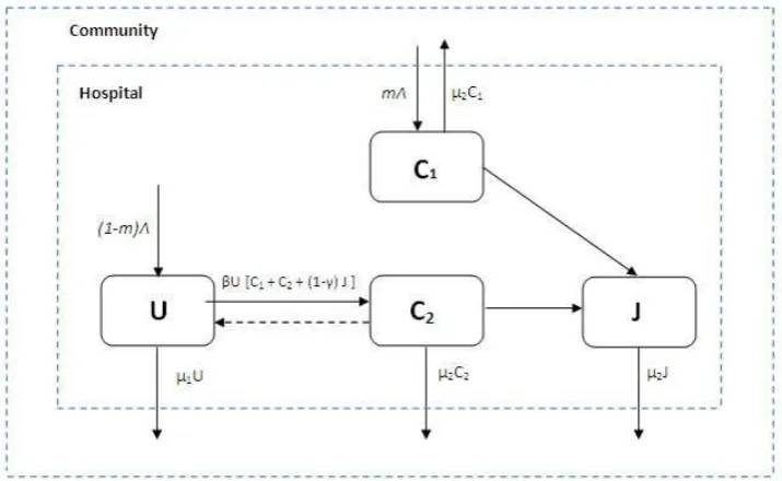
We consider a simple compartmental model in which patients in a hospital unit are classiﬁed as either uncolonized 𝑈(𝑡), VRE colonized𝐶(𝑡) or VRE colonized in isolation

𝐽(𝑡), as depicted in the compartmental schematic of Figure 1. A description of the variables and parameters used in our model are given in Table 1. The model assumptions are listed in the following itemization.

1. Compartments are homogeneous that is, each patient is considered equally likely to be in contact with a health care worker in any time interval, equally likely to be VRE colonized, and, if VRE colonized at a given time, equally likely to transmit the pathogen at a given time.

2. The transition from one compartment to another follows an exponential distribu-tion and the expected mean duradistribu-tion within a compartment is given by the inverse of the parameters of the exponential distribution.

3. Patients are admitted to the hospital unit at a rate Λ per day and some fraction m are already VRE colonized. Therefore VRE colonized patients can enter the hospital at a rate𝑚Λ and remain for an average duration of time 1/(𝜇2+𝛼). 4. New uncolonized patients enter the hospital at a rate (1−m)Λ.

5. Isolated patients remain admitted for an average duration of time 1/𝜇2.

6. It is assumed that an average patient in the population makes𝛽𝑁 eﬀective contacts (i.e., contact suﬃcient to lead to VRE colonization) with other patients per unit time through health care workers, where 𝑁 is the total population size. This assumption of a rate of contact per infective proportional to the population size

𝑁 is called mass action incidence.

7. The hand-hygiene policy applied to health care workers on isolated VRE colonized patients reduces infectivity by a factor of𝛾 (0< 𝛾 <1). This assumption means that isolated VRE colonized patients make fewer contacts than regular patients, so transmission of the bacteria by these isolated members has an infectivity factor (1−𝛾).

(17)

Figure 1: Compartmental VRE model

time per infective is (𝛽𝑁)(𝑈/𝑁). This yields a rate of new VRE colonization (𝛽𝑁)(𝑈/𝑁) [𝐶+ (1−𝛾)𝐽] =𝛽𝑈[𝐶+ (1−𝛾)𝐽].

9. It is assumed VRE colonization periods last from weeks to months. However, because spontaneous decolonization occurs infrequently, clearance of the bacteria is not considered in the model.

10. VRE colonized patients are not treated for VRE.

11. It is assumed that all patients on admission are swab tested for VRE.

12. The waiting time for the results of the swab-test cultures is assumed to be the same for all patients in any time period. After results are returned, VRE colonized patients are moved into isolation at a rate𝛼.

13. As a simpliﬁcation, we assume that the total number of patients remains ﬁxed (i.e., overall admission rate equals overall discharge rate, Λ = 𝜇1𝑈 +𝜇2(𝐶+𝐽) and VRE colonization confers no additional mortality. Then the total population of patients can be written as 𝑁 =𝑈 +𝐶+𝐽.

3.3 The VRE stochastic model

We model the dynamic of the VRE colonization of patients in a hospital unit as a con-tinuous time Markov Chain (MC) with discrete state space embedded inℝ3. Therefore,

(18)

Table 1: Model Parameters

Variables Description Units

𝑈(t) Number of uncolonized patients Individuals

𝐶(t) Number of VRE colonized patients Individuals

𝐽(t) Number of VRE colonized patients in isolation Individuals

Parameters Description Units

Λ Patients admission rate Individuals/day

𝑚 VRE colonized patients on admission rate Dimensionless

𝛽 Eﬀective contact rate 1/day

𝛾 HCW hand hygiene compliance rate Dimensionless

𝛼 Patient Isolation rate 1/day

𝜇1 Uncolonized patients discharged rate 1/day

𝜇2 VRE colonized patients discharged rate 1/day

to another is described by the equations

𝑃{𝑈(t+dt) =𝑖−1, 𝐶(t+dt) =𝑗+ 1, 𝐽(t+dt) =𝑘∣𝑈(t) =𝑖, 𝐶(t) =𝑗, 𝐽(t) =𝑘}

=𝑚𝜇1𝑈dt+𝛽𝑈[𝐶+ (1−𝛾)𝐽]dt+o(dt), (30)

𝑃{𝑈(t+dt) =𝑖, 𝐶(t+dt) =𝑗+ 1, 𝐽(t+dt) =𝑘−1∣𝑈(t) =𝑖, 𝐶(t) =𝑗, 𝐽(t) =𝑘}

=𝑚𝜇2𝐽dt+o(dt), (31)

𝑃{𝑈(t+dt) =𝑖+ 1, 𝐶(t+dt) =𝑗−1, 𝐽(t+dt) =𝑘∣𝑈(t) =𝑖, 𝐶(t) =𝑗, 𝐽(t) =𝑘}

= (1−𝑚)𝜇2𝐶dt+o(dt), (32)

𝑃{𝑈(t+dt) =𝑖+ 1, 𝐶(t+dt) =𝑗, 𝐽(t+dt) =𝑘−1∣𝑈(t) =𝑖, 𝐶(t) =𝑗, 𝐽(t) =𝑘}

= (1−𝑚)𝜇2𝐽dt+o(dt), (33)

𝑃{𝑈(t+dt) =𝑖, 𝐶(t+dt) =𝑗−1, 𝐽(t+dt) =𝑘+ 1∣𝑈(t) =𝑖, 𝐶(t) =𝑗, 𝐽(t) =𝑘}

=𝛼𝐶dt+o(dt), (34)

𝑃{𝑈(t+dt) =𝑖, 𝐶(t+dt) =𝑗, 𝐽(t+dt) =𝑘∣𝑈(t) =𝑖, 𝐶(t) =𝑗, 𝐽(t) =𝑘}

= (1−𝑚)𝜇1𝑈dt+𝑚𝜇2𝐶dt+ [1−(Λ +𝛽𝑈[𝐶+ (1−𝛾)𝐽] +𝛼𝐶)]dt+o(dt). (35)

We present next a model description underlying these equations. In the VRE epi-demic model a constant population is assumed in which the hospital remains full for all t (Assumption (13)). Hence, the admission of a patient in either compartments 𝑈

(19)

the probability of entering compartment 𝐶 by either an admission (due to a discharge in compartment 𝑈) or by eﬀective colonization. Equation (3.2) is the probability of entering compartment𝐶 by an admission due to a discharge in𝐽. Equation (3.3) is the probability of admission to compartment 𝑈 by a discharge in𝐶. Equation (3.4) is the probability of admission into compartment𝑈 by a discharge in𝐽. Equation (3.5) is the probability of moving a VRE colonized patient into isolation. Finally, Equation (3.6) is the probability that none of the states changes due to: an uncolonized patient being discharged and replaced back into the 𝑈 compartment, or a VRE colonized patient in

𝐶 being discharged and replaced back into the 𝐶 compartment, or no event occurs. When dividing these probabilities by dt and taking the limit when dt tends to 0+, we obtain the rates of transitions that are given in Table 2. Since this is a stochastic model, the rates represent the mean number of transitions that can be expected in a given period, with the actual numbers distributed about these means. Hence, the rates determine the frequencies of occurrence through time for the transitions or events.

Letting 𝑅𝑖(t) for 𝑖= 1, ...,6, be the number of times the 𝑖𝑡ℎ transition has occurred by timet. Then, the state of the system at time t can be written as

𝑈(𝑡) = 𝑈(0)−𝑅1(𝑡)−𝑅4(𝑡)−𝑅5(𝑡) + (1−𝑚)(𝑅1(𝑡) +𝑅2(𝑡) +𝑅3(𝑡))

𝐶(𝑡) = 𝐶(0)−𝑅2(𝑡) +𝑅4(𝑡) +𝑅5(𝑡)−𝑅6(𝑡) +𝑚(𝑅1(𝑡) +𝑅2(𝑡) +𝑅3(𝑡))

𝐽(𝑡) = 𝐽(0)−𝑅3(𝑡) +𝑅6(𝑡), (36)

where𝑅𝑖(𝑡) is a counting process with intensity 𝜆𝑖(𝑈(𝑡), 𝐶(𝑡), 𝐽(𝑡)) given by

𝑅𝑖(𝑡) =𝑌𝑖 (∫ 𝑡

0

𝜆𝑖(𝑈(𝑠), 𝐶(𝑠), 𝐽(𝑠))𝑑𝑠 )

, 𝑖= 1, ...,6, (37)

with 𝑌𝑖 as independent unit Poisson processes. Note that the state of the system is

{𝑈(𝑠), 𝐶(𝑠), 𝐽(𝑠)} and hence each 𝜆𝑖(𝑈(𝑠), 𝐶(𝑠), 𝐽(𝑠)) is constant between transition times. Also, note that sample paths 𝑟𝑖(𝑡) of 𝑅𝑖(t) are given in terms of sample paths

{𝑢(𝑡), 𝑐(𝑡), 𝑗(𝑡)}of {𝑈(𝑡), 𝐶(𝑡), 𝐽(𝑡)} by

𝑟𝑖(𝑡) =𝑌𝑖 (∫ 𝑡

0

𝜆𝑖(𝑢(𝑠), 𝑐(𝑠), 𝑗(𝑠))𝑑𝑠 )

, 𝑖= 1, ...,6. (38)

3.4 The VRE deterministic model

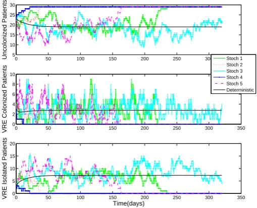
We are also interested in the deterministic approximation of the continuous time discrete state Markov Chain model already described when the population sizeN is large. The deterministic approximation is based on Kurtz’s approximation in mean theory [29].

(20)

Table 2: Transition rates

Event Eﬀect Transition rate

Discharge of uncolonized patient (U,C,J)=(i-1,j,k) 𝜆1=𝜇1𝑈

Discharge of VRE colonized patient (U,C,J)=(i,j-1,k) 𝜆2=𝜇2𝐶

Discharge of VRE colonized patient

in isolation (U,C,J)=(i,j,k-1) 𝜆3=𝜇2𝐽

Patient colonization due to VRE

colonized patients (U,C,J)=(i-1,j+1,k) 𝜆4=𝛽𝑈 𝐶

Patient colonization due to VRE

colonized patients in isolation (U,C,J)=(i-1,j+1,k) 𝜆5=𝛽(1−𝛾)𝑈 𝐽

Isolation of VRE colonized patient (U,C,J)=(i,j-1,k+1)) 𝜆6=𝛼𝐶

Admission of uncolonized patient U=i+1 (1−m)(𝜆1+𝜆2+𝜆3)

Admission of VRE colonized patient C=j+1 m(𝜆1+𝜆2+𝜆3)

We rescale the rates𝜆𝑖 for𝑖= 1, ...,6 as follows:

𝜆1 =𝜇1𝑢(𝑡) =𝑁 𝜇1𝑥(𝑡), 𝜆4 =𝛽𝑢(𝑡)𝑐(𝑡) =𝑁2𝛽𝑥(𝑡)𝑦(𝑡),

𝜆2 =𝜇2𝑐(𝑡) =𝑁 𝜇2𝑦(𝑡), 𝜆5 =𝛽(1−𝛾)𝑢(𝑡)𝑗(𝑡) =𝑁2𝛽(1−𝛾)𝑥(𝑡)𝑧(𝑡),

𝜆3 =𝜇2𝑗(𝑡) =𝑁 𝜇2𝑧(𝑡), 𝜆6 =𝛼𝑐(𝑡) =𝑁 𝛼𝑦(𝑡).

Using these rates we can obtain an approximation for the sample paths 𝑟𝑖(𝑡) of (38) by applying the SLLN for the Poisson Process (i.e., 𝑌(𝑁 𝜇)/𝑁 ≈𝜇). Therefore, we ﬁnd

𝑟𝑁₁ (𝑡) = 𝑟1(𝑡)

𝑁 =

1

𝑁𝑌1

(∫ 𝑡 0

𝜆1(𝑢(𝑠))𝑑𝑠 )

= 1

𝑁𝑌1

(

𝑁

∫ 𝑡 0

𝜇1𝑥(𝑠)𝑑𝑠 )

≈ ∫ 𝑡

0

𝜇1𝑥(𝑠)𝑑𝑠. (39)

(21)

stochastic equations (36) via the SLLN are given by

𝑥𝑁(𝑡) =𝑥(0)−𝑟𝑁₁ (𝑡)−𝑟₄𝑁(𝑡)−𝑟₅𝑁(𝑡) + (1−𝑚)(𝑟₁𝑁(𝑡) +𝑟𝑁₂ (𝑡) +𝑟₃𝑁(𝑡)) ≈𝑥(0)−

∫ 𝑡 0

𝜇1𝑥(𝑠)𝑑𝑠− ∫ 𝑡

0

𝑁 𝛽𝑥(𝑠)𝑦(𝑠)𝑑𝑠− ∫ 𝑡

0

𝑁 𝛽(1−𝛾)𝑥(𝑠)𝑦(𝑠)𝑑𝑠

+ ∫ 𝑡

0

(1−𝑚)(𝜇1𝑥(𝑠) +𝜇2(𝑦(𝑠) +𝑧(𝑠)))𝑑𝑠

𝑦𝑁(𝑡) =𝑦(0)−𝑟𝑁₂ (𝑡) +𝑟𝑁₄ (𝑡) +𝑟₅𝑁(𝑡)−𝑟𝑁₆ (𝑡) +𝑚(𝑟𝑁₁ (𝑡) +𝑟𝑁₂ (𝑡) +𝑟₃𝑁(𝑡)) ≈𝑦(0)−

∫ 𝑡 0

𝜇2𝑦(𝑠)𝑑𝑠+ ∫ 𝑡

0

𝑁 𝛽𝑥(𝑠)𝑦(𝑠)𝑑𝑠+ ∫ 𝑡

0

𝑁 𝛽(1−𝛾)𝑥(𝑠)𝑧(𝑠)𝑑𝑠

− ∫ 𝑡

0

𝛼𝑦(𝑠)𝑑𝑠+ ∫ 𝑡

0

𝑚(𝜇1𝑥(𝑠) +𝜇2(𝑦(𝑠) +𝑧(𝑠)))𝑑𝑠

𝑧𝑁(𝑡) =𝑧(0)−𝑟₃𝑁(𝑡) +𝑟₆𝑁(𝑡) ≈𝑧(0)−

∫ 𝑡 0

𝜇2𝑧(𝑠)𝑑𝑠+ ∫ 𝑡

0

𝛼𝑦(𝑠)𝑑𝑠. (40)

Upon approximating{𝑥𝑁(𝑡), 𝑦𝑁(𝑡), 𝑧𝑁(𝑡)}by{𝑥(𝑡), 𝑦(𝑡), 𝑧(𝑡)}and diﬀerentiating the above equations we obtain the ordinary diﬀerential equations

𝑑𝑥(𝑡)

𝑑𝑡 =−𝜇1𝑥(𝑡)−𝛽𝑁 𝑥(𝑡)𝑦(𝑡)−𝛽𝑁(1−𝛾)𝑥(𝑡)𝑧(𝑡) + (1−𝑚)(𝜇1𝑥+𝜇2(𝑦+𝑧)) 𝑑𝑦(𝑡)

𝑑𝑡 =−𝜇2𝑦(𝑡) +𝛽𝑁 𝑥(𝑡)𝑦(𝑡) +𝛽𝑁(1−𝛾)𝑥(𝑡)𝑧(𝑡)−𝛼𝑦(𝑡) +𝑚(𝜇1𝑥+𝜇2(𝑦+𝑧)) 𝑑𝑧(𝑡)

𝑑𝑡 =−𝜇2𝑧(𝑡) +𝛼𝑦(𝑡), (41)

with initial conditions 𝑥(0) =𝑥0,𝑦(0) =𝑦0, and 𝑧(0) =𝑧0.

To facilitate comparison with the MC model, we let 𝑈(𝑡) = 𝑁 𝑥(𝑡), 𝐶(𝑡) = 𝑁 𝑦(𝑡), and 𝐽(𝑡) =𝑁 𝑧(𝑡). Then, the system of ordinary diﬀerential equations which provides an approximation to averages over sample paths of {𝑈((𝑡), 𝐶(𝑡), 𝐽(𝑡)} is described by

𝑑𝑈(𝑡)

𝑑𝑡 = (1−𝑚)[𝜇1𝑈(𝑡) +𝜇2(𝐶(𝑡) +𝐽(𝑡))]−𝛽𝑈(𝑡)[𝐶(𝑡) + (1−𝛾)𝐽(𝑡)]−𝜇1𝑈(𝑡) 𝑑𝐶(𝑡)

𝑑𝑡 =𝑚[𝜇1𝑈(𝑡) +𝜇2(𝐶(𝑡) +𝐽(𝑡))] +𝛽𝑈(𝑡)[𝐶(𝑡) + (1−𝛾)𝐽(𝑡)]−(𝛼+𝜇2)𝐶(𝑡) 𝑑𝐽(𝑡)

𝑑𝑡 =𝛼𝐶(𝑡)−𝜇2𝐽(𝑡), (42)

(22)

3.4.1 Steady states and the basic reproductive number

In the absence of VRE colonization on admission (i.e., 𝑚 = 0) there are two steady states. The one indicating the absence of VRE colonization or the VRE-free equilibrium denoted by 𝐸0, and the other indicating the presence of VRE colonization denoted by 𝐸𝑒_{. The former is used to calculate the basic reproductive number} _ℛ

0, known in epidemiological models as the average number of secondary cases caused by an infected individual during his/her infectious period when introduced in a completely disease-free population.

Since we have a constant population, for convenience the Model (42) can be reduced to a two dimension system given by

𝑑𝐶(𝑡)

𝑑𝑡 = 𝛽𝑈(𝑡)[𝐶(𝑡) + (1−𝛾)𝐽(𝑡)]−(𝛼+𝜇2)𝐶(𝑡) 𝑑𝐽(𝑡)

𝑑𝑡 = 𝛼𝐶(𝑡)−𝜇2𝐽(𝑡) 𝑈(𝑡) = 𝑁−𝐶(𝑡)−𝐽(𝑡)

𝐶(𝑡0) = 𝐶0

𝐽(𝑡0) = 𝐽0. (43)

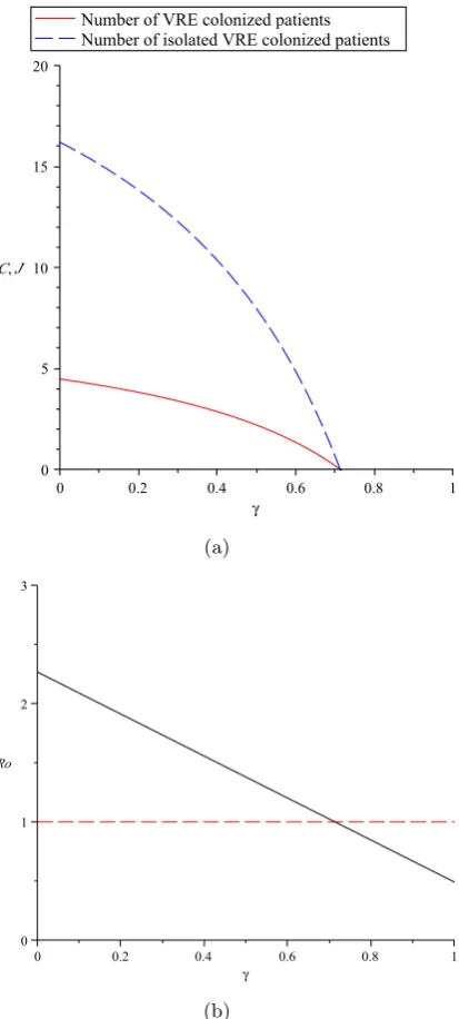
The basic reproductive number The basic reproductive numberℛ0 can be deﬁned

as the average number of secondary VRE colonized patients generated by a primary case VRE colonized patient in a VRE-free hospital unit. Hence, this quantity plays an important role in determining the possible limiting behaviors of the model, i.e., to what extent VRE colonizations become or remain endemic in a hospital unit population. Assuming that 𝐶 and 𝐽 are infective classes and using methodology in [27], we have

ℱ = [

𝛽𝑈[𝐶+ (1−𝛾)𝐽] 0

]

𝒱 = [

(𝛼+𝜇2)𝐶

−𝛼𝐶+𝜇2 ]

,

where the vector ℱ represents all new colonizations and the vector 𝒱 represents the transitions out of each compartment. Note that progression from C to J is not considered to be new colonization but rather the progression of a VRE colonized patient to the isolation compartment. Since the VRE-free equilibrium is 𝐸0 = (𝐶0, 𝐽0) = (0,0)𝑇 we have

𝐹 = [

𝛽𝑁 𝛽𝑁(1−𝛾)

𝛼 0

]

𝑉 = [

𝛼+𝜇2 0 −𝛼 𝜇2

]

,

(23)

𝐹 𝑉−1 = [

𝛽𝑁 𝛼+𝜇2 +

𝛽𝑁(1−𝛾)𝛼 (𝛼+𝜇2)𝜇2

𝛽𝑁(1−𝛾) 𝜇2

0 0

]

.

Thereforeℛ₀ is given by the spectral radius of the matrix𝐹 𝑉−1 (i.e.,ℛ₀ =𝜌(𝐹 𝑉−1)):

ℛ0 =

𝛽𝑁 𝛼+𝜇2

+ 𝛼

𝛼+𝜇2

𝛽𝑁(1−𝛾)

𝜇2

. (44)

Each term in ℛ₀ has an epidemiological interpretation. We may argue that a VRE colonized patient in a totally susceptible hospital unit population causes 𝛽𝑁 new col-onizations in unit time. The quantity _𝛼₊1_𝜇

2 is the average time that a VRE colonized

patient spends in the compartment𝐶, and this multiplied by𝛽𝑁 are the average number of individuals recruited in this class. This indeed, roughly speaking, is the basic repro-ductive number for a VRE compartmental model including only the ﬁrst infective class

𝐶, i.e., ℛ₀(𝑈 →𝐶). The quantity _𝛼₊𝛼_𝜇

2 is the fraction of VRE colonized patients that

are isolated. While in the isolation compartment 𝐽, the number of new VRE coloniza-tions caused in unit time is 𝛽𝑁(1−𝛾) and the mean time in isolation compartment is

𝜇2. Therefore, the second term in (44) represents the average number of secondary VRE colonizations, patients recruited to 𝐶, by individuals who progressed to the isolation compartment𝐽.

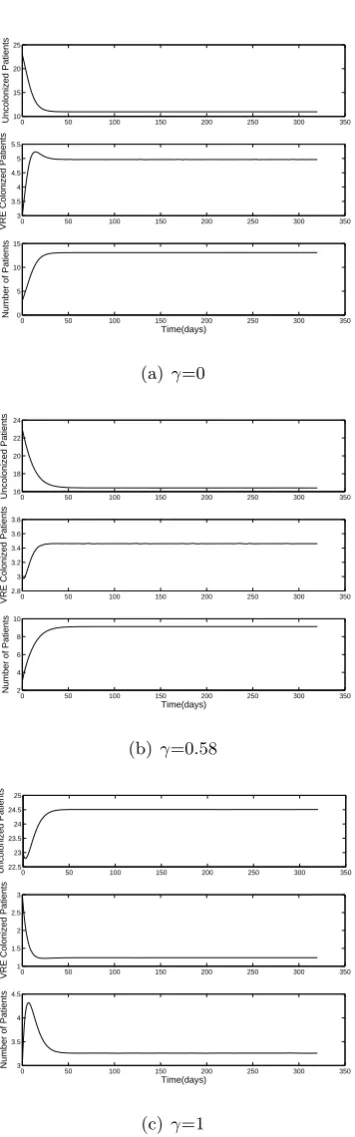
The fact that ℛ₀ is dependent on 𝛾 leads us to conclude that health HCW hand-hygiene encouragement has an eﬀect controlling the epidemic of VRE. Note that if we have the case 𝛾= 1, a 100% HCW hand hygiene compliance, this term cancels out and does not contribute to ℛ₀. Hence, with a high compliance rate the VRE incidence can be attributed more to the ﬁrst infective class 𝐶 than to the second infective class 𝐽.

The VRE-free equilibrium. It is given by

𝐸0 = (𝐶0, 𝐽0)𝑇 = (0,0)𝑇. (45)

Proposition 3.1. Let 𝐸0= (0,0) be the VRE-free equilibrium of (43), then it is locally

asymptotically stable if and only if ℛ0<1.

Proof. The Jacobian given from the linearization at the VRE-free equilibrium point is:

𝐽(0,0) = [

𝛽𝑁−(𝛼+𝜇2) 𝛽𝑁(1−𝛾)

𝛼 −𝜇2

]

.

(24)

Proposition 3.2. Let 𝐸0= (0,0)be the VRE-free equilibrium of (43), then it is globally stable if𝛽𝑁 < 𝜇2.

Proof. Let 𝑉 =𝐶+𝐽 be the Lyapunov function (i.e., a continuously diﬀerentiable real valued function) and 𝑥∗ be the VRE-free equilibrium point. We have

1. 𝑉(𝑥)>0 for all𝑥=∕ 𝑥∗, and 𝑉(𝑥∗) = 0,

2. If𝛽𝑁 < 𝜇2, then 𝑑𝑉_𝑑𝑡 <0 for all 𝑥∕=𝑥∗,

𝑑𝑉 𝑑𝑡 =

𝑑𝐶 𝑑𝑡 +

𝑑𝐽 𝑑𝑡

=𝛽𝑈[𝐶+ (1−𝛾)𝐽]−𝜇2(𝐶+𝐽)

⩽𝛽𝑈(𝐶+𝐽)−𝜇2(𝐶+𝐽)

⩽(𝛽𝑁 −𝜇2)(𝐶+𝐽), since 𝑈 ⩽𝑁.

Thus,𝑥∗ is globally stable for all initial conditions, and 𝑥(𝑡)→𝑥∗ as𝑡→ ∞.

The endemic equilibrium. It is given by 𝐸𝑒= (𝐶𝑒, 𝐽𝑒), where

𝐶𝑒= 𝜇

2 2

𝛽[𝛼(1−𝛾) +𝜇2]

[ℛ₀−1] (46)

𝐽𝑒= 𝛼𝜇2

𝛽[𝛼(1−𝛾) +𝜇2][ℛ0−1]. (47) The existence andlocal stability of the endemic equilibrium is conditioned on ℛ₀ >1.

Proposition 3.3. Let 𝐸𝑒 = (𝐶𝑒, 𝐽𝑒) be the VRE-endemic equilibrium of (43), then it

is locally asymptotically stable if and only if ℛ0 >1.

Proof. The Jacobian given from the linearization at the VRE-endemic equilibrium point is:

𝐽(𝐶𝑒, 𝐽𝑒) = [

−(2𝜇2(ℛ0−1)−𝛽𝑁+𝛼+𝜇2) −(2𝜇2(ℛ0−1)−𝛽𝑁(1−𝛾))

𝛼 −𝜇2

]

.

(25)

3.5 Parameters estimated directly from the VRE surveillance data

In this section we estimate the parameters from the VRE model discussed previously using the VRE surveillance data corresponding to the oncology unit and the general unit. The isolation procedure in these units corresponds to the one assumed in the general VRE epidemic model.

In an attempt to estimate the fraction (𝑚) of patients that are colonized on admission, in both units we found inconsistencies in the reported prevalence of VRE on admission (the summaries of admitted patients did not match the actual data). Also, in an attempt to estimate the initial conditions (𝑆0, 𝐶0, 𝐽0) from the data reported on the ﬁrst day of data collection (January 3, 2005 for the oncology unit and October 1, 2004 for the general unit), we found that only the number of VRE colonized patients in isolation was reported. Hence, the initial conditions for 𝑆0 and 𝐶0 cannot be easily estimated. Another parameter that is of interest and can not be estimated directly from the data is the VRE transmission rate (𝛽). As a result, the fraction of patients that are colonized on admission, the initial conditions, and the transmission rate are estimated using inverse problem methodology discussed in the following section. In Table 3 we present the assumed initial values of these parameters needed for inverse problem purposes.

Colonized isolation rate (𝛼): VRE colonized patients were put into isolation as soon as the admission swab result were known to be positive. It was told that the test will be back in 2 days but it is possible that this test will be back after 5 days. Therefore, we set 1/𝛼= (2 + 5)/2 = 3.5, giving the isolation rate 𝛼= 0.29.

Health care worker hand-hygiene compliance (𝛾): Infection control measures were implemented in the form of health care worker hand-hygiene before and after patients contact by the use of gloves and gowns, and washing the hands. In Figure 2 we present the level of compliance at three months interval. For this study we are going to consider the health care worker before patient contact compliance as a better estimator for the parameter𝛾. The mean compliance was 50.63% for the general unit, and 57.56% for the oncology unit.

Discharge rate: We do not consider same day discharges. In the oncology unit VRE colonized patients had a mean length of stay of 13.15 days (std=18.28) compared with 6.27 (std=6.80) for the uncolonized patients. In the general ward unit, VRE-colonized patients had a mean stay of 9 (std=13.05) compared with 5 (std=6.89) for the un-colonized patients. In both units, the means between VRE un-colonized and unun-colonized patients were statistically significant different suggesting to us the consideration of differ-ent discharge rates. For the oncology unit, we take 1/𝜇1= 6.27 and 1/𝜇2= 13.15 giving

𝜇1= 0.16 and 𝜇2= 0.08. On the other hand, for the general unit we take 1/𝜇1 = 5 and 1/𝜇2 = 9 giving𝜇1 = 0.20 and𝜇2 = 0.11.

(26)

(27)

1 2 3 4 5 6 7 8 0

500 1000 1500 2000 2500

Frecuency

Length of Stay (in groups of days)

Figure 3: Distribution of length of stay in groups of days: 1 := 1-7 days, 2 := 8-14 days, 3 := 15-21 days, 4 := 22-28 days, 5 := 29-35 days, 6 := 36-42 days, 7 := 43-49 days, 8 := 50 days or more.

staying in the hospital for a considerable amount of time, some of whom are present for at least 7 weeks (50 days). This is expected, as the needs of patients suﬀering from cancer are quite complex in nature, possibly requiring additional rehabilitation and care. The length of hospital stay distribution ﬁts an exponential distribution (Anderson-Darling p-value = 0.2043). Similar results are found for the general unit (Anderson-Darling p-value = 0.2627).

3.6 Inverse problem

As a result of the previous section, it is of interest to estimate the initial conditions, the fraction of patients that are colonized on admission, and the VRE transmission rate, i.e., 𝜃= (𝐽0, 𝐶0, 𝑚, 𝛽). The ODE model (42) along with the surveillance data collected for the oncology and general units are used to estimate the parameters via the nonlinear least squares optimization methods described in Section 2.

The VRE model (51) can be rewritten in the general vector form (1) with 𝑥(𝑡) = (𝑈(𝑡), 𝐶(𝑡), 𝐽(𝑡))𝑇 and observational process as

𝑦(𝑡𝑗) = [

0 0 1 ] ⎡ ⎣

𝑈(𝑡𝑗)

𝐶(𝑡𝑗)

𝐽(𝑡𝑗) ⎤

(28)

Table 3: Parameters values (some values are assumed for optimization purposes)

Initial Conditions Oncology Unit (N=37) General Unit (N=29) Source

𝑈(t0) 29 23 Assumed

𝐶(t0) 4 3 Assumed

𝐽(t0) 4 3 data

Parameters

Λ 𝜇1𝑈(t) +𝜇2(𝐶(t) +𝐽(t)) 𝜇1𝑈(t) +𝜇2(𝐶(t) +𝐽(t))

-𝑚 0.04 0.04 Assumed

𝛽 0.001 0.001 Assumed

𝛾 0.58 0.51 data

𝛼 0.29 0.29 data

𝜇1 0.16 0.20 data

𝜇2 0.08 0.11 data

Note that the relationship between number of patients in the isolation compartment (𝐽) and time is described by a nonlinear function in its parameters. The algorithm that searches all possible parameter combinations in our problem is:

1. Combinatorial search. For a ﬁxed 𝑗 = 1, ...,8, and hence ﬁxed 𝑝, calculate the

set

𝑆𝑝 ={𝜃= (𝑞1, ..., 𝑞𝑗)∈ℝ𝑝∣𝑞𝑘 ∈ ℵ, 𝑞𝑘∕=𝑞𝑙 ∀𝑘, 𝑙= 1, ..., 𝑗}

where 𝑞𝑘 = {𝛼, 𝛾, 𝜇1, 𝜇2, 𝐽0, 𝐶0, 𝑚, 𝛽} and the set 𝑆𝑝 collects all the parameter vectors obtained from the combinatorial search;

2. Full rank test. Calculate the set of feasible parameters Θ𝑝 as

Θ𝑝 ={𝜃∣𝜃 ∈ 𝑆𝑝 ⊂ℝ𝑝, 𝑟𝑎𝑛𝑘(𝜒(𝜃) = 𝑝)}. Calculate the condition number deﬁned

by

𝑘(𝜒(𝜃)) = 𝑠1

𝑠𝑝 ;

3. Standard error test. For every 𝜃 ∈ Θ𝑝, calculate a vector of coeﬃcients of

variation 𝐶𝑉(𝜃)∈_ℝ𝑝 _by

𝐶𝑉𝑖 = √

(∑ (𝜃)𝑖𝑖

𝜃𝑖

,

for 𝑖 = 1, ..., 𝑝 and ∑

(𝜃) = 𝜎2

0[𝜒(𝜃)𝑇𝜒(𝜃)]−1 ∈ ℝ𝑝×𝑝. Calculate the parameter selection score as𝜐(𝜃) =∣𝐶𝑉(𝜃)∣.

3.6.1 Optimization algorithm testing with synthetic data

(29)

corresponding model solution, 𝑓(𝑡𝑗, 𝜃0) =𝐽(𝑡𝑗, 𝜃0). The statistical model that captures the variability is taken as

𝑦𝑗 =𝑓(𝑡𝑗, 𝜃0) +𝜎𝑧𝑗 (49)

where𝑧𝑗 is a standard normal variable (i.e., 𝑧𝑗 ∼𝑁(0,1)) and𝜎 is the constant

variabil-ity. The magnitude of𝜎 determines how much noise is added. A low value indicates that the data points tend to be very close to the same value (the mean), while high values indicates that the data are “spread out” over a large range of values. Therefore, we can expect that 95% of the time, numbers generated from this distribution will fall in the interval [−1.96𝜎,1.96𝜎]. To this end, we look at the standard error as one indication of the ability of the algorithm to estimate the parameters using the synthetic data set.

The OLS and GLS optimization were solved with MATLAB routine 𝑙𝑠𝑞𝑛𝑜𝑛𝑙𝑖𝑛 for n=500. Parameter upper bounds are taken as

(𝛼, 𝛾, 𝜇1, 𝜇2, 𝐽0, 𝐶0, 𝑚, 𝛽) = (0.5,1,1,1, 𝑁, 𝑁,1,1)

and lower bounds are set to zero. Note that the upper bound for 𝛼 is 0.5 because the method for VRE detection takes at least 2 days. The model solutions𝑓(𝑡𝑗;𝜃0) =𝐽(𝑡𝑗;𝜃0) are generated with initial conditions and parameter values for the oncology unit as described in Table 3 (which are assumed to be the true values). By introducing variability levels such as𝜎 = 0,𝜎 = 0.01,𝜎= 0.05, and𝜎= 0.1 in the model solutions the reliability of the algorithm and hence that of estimates are explored. Note that for this purpose, there is no need to test the algorithm using the general unit values. Also, even though we are adding constant variability to the synthetic data, the GLS optimization algorithm is tested with this data. This is because we are investigating how the noise aﬀects the standard deviation and not how meaningful they are.

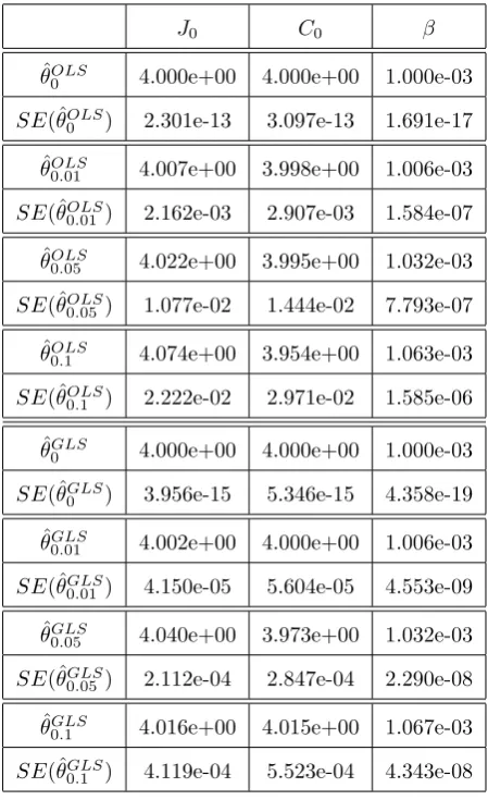
In Tables 4, 5, and 6 we summarize the results for the inverse problems for 𝜃 = (𝐽0, 𝐶0, 𝛽), 𝜃 = (𝐽0, 𝐶0, 𝑚, 𝛽), and 𝜃 = (𝛼, 𝐽0, 𝐶0, 𝑚, 𝛽) using an OLS and a GLS opti-mization formulation. Results indicates that both algorithms appear to be reliable for the estimation of the parameters since the estimated values are close to their true values. Note that as𝜎increases the corresponding standard errors increases. This indicates that the reliability of both algorithms in estimating the parameters may depend on the ob-servational error in the data. Similar results were obtained for the other types of inverse problems formulations.

3.6.2 Subset selection results using the oncology unit surveillance data

To carry out the subset selection algorithm with the oncology unit surveillance data we assumed parameter values described in Table 3. Since we are interested in estimating the initial conditions, transmission rate, and the fraction of patients that are already colonized on admission, when𝑝= 4 the only parameter combination considered is that of 𝜃 = (𝐽0, 𝐶0, 𝑚, 𝛽). When 𝑝 = 1,2,3 the only parameters considered are 𝜃 = (𝛽),

(30)

Table 4: OLS and GLS optimization algorithm testing for𝜃= (𝐽0, 𝐶0, 𝛽) using synthetic data. The model was ﬁt to the synthetic data with levels of noise: 𝜎 = 0,0.01,0.05,and 0.1. Subscripts in𝜃𝜎 denote the level of noise in the synthetic data.

𝐽0 𝐶0 𝛽

ˆ 𝜃𝑂𝐿𝑆

0 4.000e+00 4.000e+00 1.000e-03

𝑆𝐸(ˆ𝜃𝑂𝐿𝑆

0 ) 2.301e-13 3.097e-13 1.691e-17

ˆ

𝜃₀𝑂𝐿𝑆_.₀₁ 4.007e+00 3.998e+00 1.006e-03 𝑆𝐸(ˆ𝜃𝑂𝐿𝑆

0.01) 2.162e-03 2.907e-03 1.584e-07

ˆ 𝜃𝑂𝐿𝑆

0.05 4.022e+00 3.995e+00 1.032e-03

0.05) 1.077e-02 1.444e-02 7.793e-07

ˆ 𝜃𝑂𝐿𝑆

0.1 4.074e+00 3.954e+00 1.063e-03

𝑆𝐸(ˆ𝜃0𝑂𝐿𝑆.1 ) 2.222e-02 2.971e-02 1.585e-06

ˆ 𝜃𝐺𝐿𝑆

0 4.000e+00 4.000e+00 1.000e-03

𝑆𝐸(ˆ𝜃𝐺𝐿𝑆

0 ) 3.956e-15 5.346e-15 4.358e-19

ˆ

𝜃0𝐺𝐿𝑆.01 4.002e+00 4.000e+00 1.006e-03

0.01) 4.150e-05 5.604e-05 4.553e-09

ˆ 𝜃𝐺𝐿𝑆

0.05 4.040e+00 3.973e+00 1.032e-03

𝑆𝐸(ˆ𝜃₀𝐺𝐿𝑆_.₀₅) 2.112e-04 2.847e-04 2.290e-08 ˆ

𝜃𝐺𝐿𝑆

0.1 4.016e+00 4.015e+00 1.067e-03

(31)

Table 5: OLS and GLS optimization algorithm testing for 𝜃 = (𝐽0, 𝐶0, 𝑚, 𝛽) using synthetic data. The model was ﬁt to the synthetic data with levels of noise: 𝜎 = 0,0.01,0.05,and 0.1. Subscripts in 𝜃𝜎 denote the level of noise in the synthetic data.

𝐽0 𝐶0 𝑚 𝛽

True 𝜃 4 4 0.04 0.001

Initial𝜃 3 5 0.05 0.002

ˆ 𝜃𝑂𝐿𝑆

0 4.000e+00 4.000e+00 4.000e-02 1.000e-03

𝑆𝐸(ˆ𝜃𝑂𝐿𝑆₀ ) 8.620e-12 1.557e-11 1.611e-13 1.352e-14 ˆ

𝜃𝑂𝐿𝑆

0.01 4.004e+00 4.008e+00 4.013e-02 9.955e-04

0.01 ) 2.372e-03 4.287e-03 4.457e-05 3.735e-06

ˆ 𝜃𝑂𝐿𝑆

0.05 4.029e+00 3.992e+00 4.032e-02 1.004e-03

0.05 ) 1.102e-02 1.990e-02 2.091e-04 1.741e-05

ˆ

𝜃𝑂𝐿𝑆0.1 4.074e+00 3.945e+00 3.987e-02 1.074e-03

0.1 ) 2.271e-02 4.067e-02 4.273e-04 3.529e-05

ˆ 𝜃𝐺𝐿𝑆

0 4.000e+00 4.000e+00 4.000e-02 1.000e-03

𝑆𝐸(ˆ𝜃𝐺𝐿𝑆0 ) 1.496e-13 2.696e-13 3.145e-15 2.626e-16

ˆ 𝜃𝐺𝐿𝑆

0.01 4.003e+00 4.001e+00 4.003e-02 1.004e-03

0.01) 4.636e-05 8.350e-05 9.762e-07 8.137e-08

ˆ

𝜃𝐺𝐿𝑆₀_.₀₅ 4.009e+00 4.013e+00 4.022e-02 1.014e-03 𝑆𝐸(ˆ𝜃𝐺𝐿𝑆

0.05) 2.343e-04 4.214e-04 4.971e-06 4.118e-07

ˆ 𝜃𝐺𝐿𝑆

0.1 4.050e+00 4.011e+00 4.046e-02 1.025e-03

(32)

Table 6: OLS and GLS optimization algorithm testing for 𝜃 = (𝛼, 𝐽0, 𝐶0, 𝑚, 𝛽) using synthetic data. The model was ﬁt to the synthetic data with levels of noise: 𝜎 = 0,0.01,0.05,and 0.1. Subscripts in 𝜃𝜎 denote the level of noise in the synthetic data.

𝛼 𝐽0 𝐶0 𝑚 𝛽

ˆ 𝜃𝑂𝐿𝑆

0 2.890e-01 4.003e+00 4.136e+00 4.451e-02 1.856e-03

0 ) 2.145e-04 5.126e-04 1.674e-03 2.009e-05 1.220e-06

ˆ

𝜃𝑂𝐿𝑆₀_.₀₁ 2.895e-01 4.010e+00 4.120e+00 4.454e-02 1.872e-03 𝑆𝐸(ˆ𝜃𝑂𝐿𝑆

0.01) 1.094e-03 2.620e-03 8.517e-03 1.025e-04 6.264e-06

ˆ 𝜃𝑂𝐿𝑆

0.05 2.811e-01 4.023e+00 4.269e+00 5.080e-02 1.670e-03

0.05) 5.755e-03 1.337e-02 4.696e-02 6.381e-04 3.168e-05

ˆ 𝜃𝑂𝐿𝑆

0.1 2.899e-01 4.051e+00 4.109e+00 4.541e-02 1.880e-03

𝑆𝐸(ˆ𝜃𝑂𝐿𝑆0.1 ) 1.071e-02 2.572e-02 8.329e-02 1.033e-03 6.263e-05

ˆ 𝜃𝐺𝐿𝑆

0 2.901e-01 4.000e+00 4.095e+00 4.325e-02 1.538e-03

0 ) 3.606e-06 8.920e-06 2.854e-05 3.686e-07 2.277e-08

ˆ

𝜃𝐺𝐿𝑆0.01 2.894e-01 4.009e+00 4.130e+00 4.300e-02 1.869e-03

0.01) 2.282e-05 5.581e-05 1.836e-04 2.373e-06 1.525e-07

ˆ 𝜃𝐺𝐿𝑆

0.05 2.787e-01 4.030e+00 4.348e+00 2.360e-02 1.860e-03

𝑆𝐸(ˆ𝜃𝐺𝐿𝑆₀_.₀₅) 1.068e-04 2.581e-04 8.901e-04 5.955e-06 5.713e-07 ˆ

𝜃𝐺𝐿𝑆

0.1 2.900e-01 4.035e+00 4.189e+00 4.739e-02 1.882e-03

(33)

and condition number 𝑘(𝜒(𝜃)) for each subset of parameters when 𝑝 = 1, ...,8. Values that fall in the smallest selection score with the relative small condition number are considered the most feasible subset of parameters. Results indicate that the subsets of parameters𝜃= (𝐽0, 𝐶0, 𝑚, 𝛽) have small condition numbers and relatively small selection scores indicating that these subsets might provide low uncertainty in the parameter estimates. In Table 8 we summarize the results of 4 inverse problems corresponding to the subsets with the lowest selection scores and small condition numbers. These subsets of parameters are:

𝜃= (𝛾, 𝐽0, 𝐶0, 𝑚, 𝛽)

𝜃= (𝐽0, 𝐶0, 𝑚, 𝛽)

𝜃= (𝐽0, 𝐶0, 𝛽)

𝜃= (𝑚, 𝛽)

We analyze the results using the coefficient of variation (CV) by looking at the effect that the inclusion or exclusion of parameters has on the vector 𝜃 = (𝐽0, 𝐶0, 𝑚, 𝛽). In this subset, the standard errors for𝐽0 is about 0.4% of the estimate, for 𝐶0 it is about 0.8% of the estimate, for𝑚 it is about 1.6% of the estimate, and for𝛽 it is 0.3% of the estimate. When including 𝛾 (i.e.,𝜃= (𝛾, 𝐽0, 𝐶0, 𝑚, 𝛽)), the CV increases for almost all parameters. On the other hand, when 𝑚 is dropped or when the initial conditions are dropped, there is a reduction in the CV. Since this reduction is not significant, we can conclude that the subset 𝜃 = (𝐽0, 𝐶0, 𝑚, 𝛽) is a good choice to be estimated from the oncology surveillance data since it provides estimates with low uncertainty.

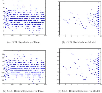
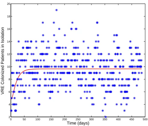
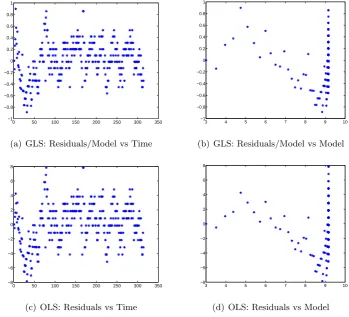
Residual plots for all subsets of parameters combinations suggested that the assump-tions of the Statistical Model (14) corresponding to the GLS procedure are satisﬁed. In particular, the residual analysis for𝜃= (𝐽0, 𝐶0, 𝑚, 𝛽) is presented in Figure 4. The OLS residual plots (a) and (b) in Figure 4 reveal a fan shaped error structure which indi-cates the nonconstant variance assumption is suspect. When GLS optimization is used instead, the residual plots (c) and (d) in Figure 4 reveals a more random error structure, suggesting that the GLS procedure was correctly used. Finally, a best ﬁt of the model solution to the oncology surveillance data is shown in Figure 5.

3.6.3 Subset selection results using the general unit surveillance data

(34)

Table 7: Subset parameter selected as a result of the selection algorithm for𝑝= 4, ...,8 using the oncology unit surveillance data with nominal parameter values described in Table 3 using the GLS optimization.

Parameter vector,𝑞 Selection score,𝜐(𝑞) Condition number,𝜅(𝜒(𝑞))

(𝛽) 1.975e-05 1.000e+00

(𝑚, 𝛽) 2.358e-03 8.070e+02

(𝐽 𝑜, 𝐶𝑜, 𝛽) 7.134e-03 8.236e+04

(𝐽 𝑜, 𝐶𝑜, 𝑚, 𝛽) 1.815e-02 9.946e+04

(𝛾, 𝐽 𝑜, 𝐶𝑜, 𝑚, 𝛽) 1.539e-01 2.253e+05

(𝛼, 𝐽 𝑜, 𝐶𝑜, 𝑚, 𝛽) 1.597e-01 1.063e+06

(𝜇1, 𝐽 𝑜, 𝐶𝑜, 𝑚, 𝛽) 1.715e+01 1.308e+08

(𝜇2, 𝐽 𝑜, 𝐶𝑜, 𝑚, 𝛽) 6.123e+03 3.695e+05

(𝛼, 𝜇1, 𝐽 𝑜, 𝐶𝑜, 𝑚, 𝛽) 6.225e+00 5.522e+06

(𝛾, 𝜇1, 𝐽 𝑜, 𝐶𝑜, 𝑚, 𝛽) 1.741e+01 1.127e+08

(𝛼, 𝜇2, 𝐽 𝑜, 𝐶𝑜, 𝑚, 𝛽) 6.315e+01 2.453e+05