ABSTRACT
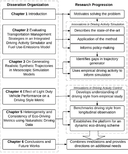
TANVIR, SHAMS. Modeling and Simulation of Driving Activity from an Energy Use- Emissions Perspective (Under the direction of Dr. Nagui Rouphail and Dr. Henry Frey). Proper understanding of driving activity at the systems level is essential to implement control technologies which improve energy efficiency and reduce emissions of harmful pollutants. The research presented in this dissertation includes methods and framework development to analyze both simulated and observed driving activities. To this end, the objectives of this research are – (a) to develop methods to efficiently evaluate transportation management strategies (TMS) in terms of emissions reduction using large scale network simulator; (b) to develop enhanced methods to generate realistic synthetic trajectories from mesoscopic traffic simulators that can faithfully represent driving activity; (c) to quantify the effect of driver and vehicle performance on the observed driving activity; and (d) to develop metrics which can distinguish the effect of driving styles on energy consumption from other confounding factors.
Post-processing methods for simulated trajectories were developed to achieve objective (b). A Savitzky-Golay filter with window width of 7 simulation time-steps and 10 smoothing iterations produced realistic simulated trajectories under congested conditions. Under uncongested condition, addition of different levels of white noise in different modes (idle, cruise, acceleration, and deceleration) of the speed trajectories generated realistic trajectories.
Variabilities in driving activities were quantified for different combinations of drivers and vehicles to attain objective (c). To this objective, we have gathered microscale vehicle activity measurements from 17 controlled real-world driving schedules and two years of naturalistic driving data from 5 drivers. We also developed a metric for driving style termed ‘envelope deviation’, which is a distribution of gaps between microscale activity (1 Hz) and
fleet average envelope. We found that there is significant inter-driver heterogeneity in driving styles when controlling for vehicle performance. The choice of vehicle was found to be not significantly altering the natural driving style of a driver.
Modeling and Simulation of Driving Activity from an Energy Use-Emissions Perspective
by Shams Tanvir
A dissertation submitted to the Graduate Faculty of North Carolina State University
in partial fulfillment of the requirements for the degree of
Doctor of Philosophy
Civil Engineering
Raleigh, North Carolina 2018
APPROVED BY:
_______________________________ _______________________________
Dr. Nagui M. Rouphail Dr. Henry Frey
Co-Chair of Advisory Committee Co-Chair of Advisory Committee
_______________________________ _______________________________
Dr. Bastian Schroeder Dr. Xuesong Zhou
DEDICATION
BIOGRAPHY
Shams Tanvir was born in Faridpur, Bangladesh to Rasida Begum and Abdul Wahab Sikder. After graduating from Notre Dame College in Dhaka, Bangladesh in 2004, he enrolled in Bangladesh University of Engineering and Technology (BUET) in Dhaka, Bangladesh. He received his BS in Civil Engineering in 2009 and MS in Civil Engineering with
specialization in Transportation Engineering in 2013 from BUET. Before joining NC State as a Ph.D. student in August 2013, he taught undergraduate courses and lab sections as a
ACKNOWLEDGMENTS
This dissertation is the culmination of the past four years of my doctoral journey. Exploring this multi-disciplinary and evolving research front has only been possible with the help of some extraordinary people.
I would like to express my deepest gratitude to my advisor, Dr. Nagui M. Rouphail for his continuous encouragement and support to explore new research ideas. He introduced me to challenging and diverse research projects and overall taught me to be an independent researcher. I am sure that his exemplary work ethics, dedication, and management skills will benefit me immensely in my future career.
I would like to thank Dr. H. Christopher Frey for teaching me rigor in research, helping me to perfect academic writing and reviewing, and epitomizing an academician. I am grateful to Dr. Bastian Schroeder, Dr. Downey Brill, and Dr. Xuesong Zhou for their
encouragement and valuable feedback on my proposal and this dissertation. I am indebted to our conversations with Dr. Sangkey Kim. Special thanks to Thomas Chase, Behzad
Aghdashi, Nabaruna Karmakar, Tai-jin Song, Kwanpyo Ko, and Ishtiak Ahmed for helping me in my research. I would like to convey my gratefulness to my parents, family members, friends, and colleagues for their support. Thanks to my wife, Rahnuma Shahrin, for
supporting and challenging me at the same time. She and my son, Sahir, sacrificed immensely to get me to this stage.
TABLE OF CONTENTS
LIST OF TABLES……….…………viii
LIST OF FIGURES………..ix
CHAPTER 1: Introduction ... 1
1.1 Background ... 2
1.2 Research Objectives ... 5
1.3 Research Scope and Limitation ... 5
1.4 Thesis Organization... 6
CHAPTER 2: Evaluating Transportation Management Strategies in an Integrated Driving Activity Simulator and Fuel Use-Emissions Model ... 8
2.1 Introduction ... 8
2.1.1 Fuel use and emissions from road traffic ... 9
2.1.2 Detrimental effects of emissions ... 10
2.1.3 Techniques for reducing fuel use and emissions from road traffic ... 11
2.1.4 Traffic simulation to assess energy use and emissions ... 13
2.1.5 Integrated traffic simulation and energy use-emissions estimation ... 14
2.1.6 Energy use and emissions estimation ... 17
2.1.7 Characterization of TMS impacts on emissions ... 23
2.2 Research Questions ... 26
2.3 Existing Methodology of Integrated DTALite and MOVES Lite Framework ... 26
2.4 Methodology for Evaluation of Transportation Management Strategies (TMS) ... 37
2.4.1 Data preparation ... 37
2.4.2 Experimental design for evaluation of TMS ... 39
2.5 Case Study ... 42
2.5.1 Description of test network ... 42
2.6 Results and discussions ... 44
2.7 Conclusions ... 49
2.8 Acknowledgments and Disclaimer ... 52
2.9 References ... 53
CHAPTER 3: On Generating Realistic Synthetic Trajectories in Mesoscopic Simulation Models ... 61
3.1 Introduction ... 61
3.1.2 Benefits of simplified trajectory generation ... 62
3.1.3 Limitations of simplified trajectory generation ... 64
3.1.4 Solving limitations of simplified trajectory generation ... 68
3.1.5 Speed of trajectory generation process ... 71
3.1.6 Simulated trajectory post-processing methods ... 71
3.1.7 Problems arising from post-processing trajectories ... 74
3.1.8 Fuel use-emissions estimation models for simulated trajectories ... 74
3.2 Research Questions ... 76
3.3 Methodology ... 76
3.3.1 Selection of study locations for empirical trajectories ... 79
3.3.2 Extraction and processing empirical trajectories ... 80
3.3.3 Simulation configuration ... 81
3.3.4 Synthetic trajectory post-processing methods ... 83
3.3.5 Selection of post-processing method and parameters ... 85
3.4 Results ... 86
3.4.1 Operating mode distributions of empirical trajectories ... 87
3.4.2 Outputs from the mesoscopic simulation module ... 90
3.4.3 Application of different post-processing methods and parameters... 92
3.4.4 Optimized parameters for post-processing methods ... 104
3.4.5 Fuel use estimations for the synthetic trajectories ... 109
3.5 Conclusions ... 110
3.6 References ... 114
CHAPTER 4: Effect of Light Duty Vehicle Performance on a Driving Style Metric ... 117
4.1 Introduction ... 117
4.1.1 Review of driving style measures ... 119
4.1.2 Review of experimental designs ... 120
4.2 Research Questions ... 122
4.3 Methods ... 122
4.3.1 Characterizing driving style ... 122
4.3.2 Comparing driving styles ... 126
4.3.3 Classifying vehicle performance ... 126
4.5 Naturalistic driving dataset... 130
4.6 Results and Discussion ... 132
4.6.1 Aggregate microscale driving statistics ... 132
4.6.2 Joint speed-acceleration distributions ... 133
4.6.3 Envelope deviation in controlled experiments ... 134
4.6.4 Envelope deviation in naturalistic studies... 140
4.7 Conclusions and Future Work ... 141
4.8 Acknowledgements ... 143
4.9 References ... 144
CHAPTER 5: Heterogeneity and Consistency of Eco-Driving Metrics using Naturalistic Driving Data ... 148
5.1 Introduction ... 148
5.2 Literature Review ... 150
5.3 Research Questions ... 153
5.4 Methodology ... 153
5.4.1 Data source... 153
5.4.2 Benchmarking driving styles through standardized fuel use ... 155
5.4.3 Eco-driving metrics development ... 157
5.4.4 Fuel efficiency score (FES) ... 158
5.4.5 Fuel use difference (FUD) ... 161
5.4.6 Characterizing heterogeneity and consistency in driving style ... 164
5.5 Results and Discussion ... 164
5.6 Conclusions and Future Work ... 171
5.7 Acknowledgements ... 173
5.8 References ... 174
CHAPTER 6 Conclusions and Future Works ... 177
6.1 Summary of Science Findings ... 177
6.1.1 Findings in simulation of driving activity ... 178
6.1.2 Findings in Control of Driving Activity ... 179
6.2 Future Works ... 180
LIST OF TABLES
Table 2.1 Performance of MOVES across different functional criteria ... 22
Table 2.2 Performance of MOVES lite across different performance criteria ... 23
Table 2.3 Selected Average emission rate for zero-age passenger cars (Frey, Yazdani-Boroujeni, Hu, Liu, & Jiao, 2013) ... 27
Table 2.4 Example sample distribution for mapping from demand type to vehicle type ... 29
Table 2.5 Vehicle age distribution by type and age (Frey et al., 2013) ... 29
Table 2.6 Network wide change for Mode Switch (MS), Fleet Replacement (FR), and Peak Spreading (PS) strategies compared to Baseline (BASE) ... 45
Table 2.7 I-540 path wide changes for Incident (INC) and corresponding variable message sign (VMS) strategy compared to Baseline (BASE) ... 45
Table 3.1 Speed-acceleration envelope from empirical observation (Liu & Frey, 2015) ... 73
Table 3.2 Definition of operating modes in EPA MOVES (EPA, 2009) ... 78
Table 3.3 Conceptual classes of distinct operating mode distributions ... 79
Table 3.4 Description of study locations for collection of observed driving activity ... 80
Table 3.5 Vehicle activity episodes determined from time-averaged simulated trajectories ... 85
Table 3.6 Range of tested signal smoothing methods and parameters ... 99
Table 3.7 Optimized parameters for freeways (𝒗𝒇 = 65 mph) ... 105
Table 3.8 Optimized parameters for arterials (𝒗𝒇 = 45 mph) ... 106
Table 3.9 Parameters and average RMSE values for micro-trip based trajectory reconstruction method ... 107
Table 4.1 Activity envelope values for real-world vehicle fleet (B. Liu & Frey, 2015) ... 124
Table 4.2 Specifications of the vehicles analyzed in the controlled experiment ... 129
Table 4.3 Specifications of the selected vehicles in the naturalistic driving experiment ... 131
Table 4.4 Example two-sample K-S test statistics, D for pairwise comparison of deviation distributions from baseline in controlled experiments... 137
LIST OF FIGURES
Figure 1.1 Dissertation organization and research framework ... 7 Figure 2.1 Modules of integrated traffic simulation and emission estimation ... 16 Figure 2.2 Systems framework of DTALite and MOVES Lite ... 28 Figure 2.3 Consistent representation of backward wave propagation in both
Newell’s kinematic wave and simplified linear car following models (Zhou et al., 2015) ... 31 Figure 2.4 Constructing microscopic vehicle trajectory from mesoscopic
simulation results (Zhou et al., 2015) ... 34 Figure 2.5 System framework and data-flow for assessing emissions impacts of
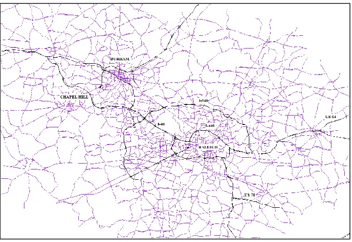
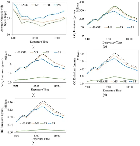
Transportation Management Strategies ... 38 Figure 2.6 Schematic of the model network ... 43 Figure 2.7 Network wide profile (a) average network speed (mph) (b) CO2 emissions
(grams) (c) NOX emissions (grams) (d) CO emissions (grams) (e) HC emissions (grams). [BASE = Baseline, MS = Mode Shift, FR = Fleet
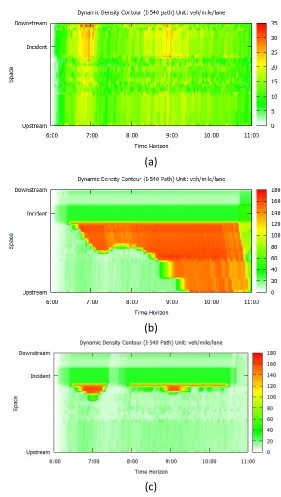
Replacement, PS = Peak Spreading] ... 46 Figure 2.8 Dynamic density contour on the I-540 path for (a) Baseline (BASE)
(b) Incident only (INC) (c) Incident with variable message sign (VMS)
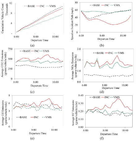
scenarios. ... 48 Figure 2.9 Path based profile on selected I-540 path (a) cumulative vehicle count
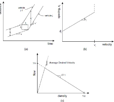
(b) average speed (mph) (c) average CO2 emissions (grams per vehicle per mile) (c) average NOX emissions (grams per vehicle per mile) (d) average CO emissions (grams per vehicle per mile) (e) average HC emissions (grams per vehicle per mile). [BASE = Baseline, INC = Incident only, VMS = Incident with variable message sign] ... 49 Figure 3.1 (a) Piecewise linear vehicle trajectories (adopted from (Newell, 2002)),
(b) relationship between velocity and spacing for an individual driver, (c) density-flow curve for Newell’s theory comparable to
macroscopic LWR fundamental diagram. ... 64 Figure 3.2 Simulated trajectory for a single vehicle in DTALite (a) speed
(b) acceleration... 65 Figure 3.3 Real world vehicle trajectories from Next Generation
Simulation (NGSIM) data (FHWA, 2015) ... 66 Figure 3.4 Speed and accelerations for real-world trajectories ... 66 Figure 3.5 Adopted approach to solve the limitations of simplified
trajectory generation ... 67 Figure 3.6 Sensitivity of fuel consumption due to application of different maximum
Figure 3.7 Instantaneous fuel consumption for VW Polo 1.4 Diesel at different speed-acceleration levels (Treiber et al., 2008) ... 70 Figure 3.8 Methodology to select post-processing methods and parameters for
synthetic trajectories generated from mesoscopic traffic simulation ... 77 Figure 3.9 Prototyping of DTALite trajectory post-processing codes in R ... 82 Figure 3.10 Operating mode distribution of empirical trajectories for freeways under
different operating conditions. The error bars represent 95% confidence interval. 𝝆 = speed-ratio. n = number of extracted trajectories to draw the distribution. 𝒗𝒇 = posted speed. ... 88 Figure 3.11 Operating mode distribution of empirical trajectories for arterials under
different operating conditions. The error bars represent 95% confidence interval. 𝝆 = speed-ratio. n = number of extracted trajectories to draw the distribution. 𝒗𝒇 = posted speed. ... 89 Figure 3.12 Outputs from the mesoscopic simulation module for a 10 link single
corridor with free-flow speed of 65 mph and backward wave speed of 12 mph. ... 91 Figure 3.13 Unsmoothed space-time trajectories for 10 simulated vehicles on a link ... 92 Figure 3.14 (a) Speed profile and (b) acceleration profile for the 7th vehicle
(shown black in Figure 3.13) ... 93 Figure 3.15 Speed-acceleration envelope for 10 simulated raw trajectories ... 93 Figure 3.16 (a) Space-time trajectories (b) speed profiles and (c) acceleration profiles
for 2nd and 8th vehicles (d) speed-acceleration envelopes (e) VSP density plot (outliers removed) for filter width 20 and 160 simulation intervals using unweighted moving average method... 94 Figure 3.17 Joint speed-acceleration distribution: simulated vs. field-observed ... 98 Figure 3.18 Modified trajectories from (a to c) smoothing space-time trajectories
using unweighted moving average with window width of 3 sec and 10 smoothing iterations (d to f) smoothing speed trajectories using unweighted moving average with window width 3 sec and 20
smoothing iterations. ... 100 Figure 3.19 Modified trajectories from (a to c) smoothing space-time trajectories
using Svitzky-Golay filter with filter length of 1/2 sec and 10 smoothing iterations. (d to f) smoothing speed trajectories using Svitzky-Golay filter with filter length 1/2 sec and 10 smoothing iterations. ... 101 Figure 3.20 Modified trajectories from (a to c) smoothing space-time trajectories
using Lowess smoothing with filter length of 1/2 sec and 10 smoothing iterations. (d to f) smoothing speed trajectories using Lowess
Figure 3.21 Modified trajectories from (a to c) speed-acceleration enveloping with enveloping zone 1/10 s and 50 iterations. (d to f) micro-trip based trajectory reconstruction for all the noise standard deviations set at 0.1 m/s. ... 104 Figure 3.22 Residual distribution for the post-processing parameter space with
different post-processing methods. The grey cells represents values
outside the plotting range. ... 108 Figure 3.23 Comparison of estimated fuel mileage for empirical and simulated
trajectories for freeways (𝒗𝒇 = 65 mph) in congested condition
(𝟎. 𝟕 ≥ 𝝆 > 𝟎. 𝟓). ... 110 Figure 4.1 Distributions of envelope deviation for standard driving cycles ... 125 Figure 4.2 (Left) i2D device connected to the vehicle. (Right) I. the device
II. antenna III. OBD-II connector cable ... 130 Figure 4.3 Cumulative Density Function of Acceleration for Dodge Caravan
(1-1-1-13) at different speed bins [n=15,450] ... 132 Figure 4.4 Joint speed-acceleration distribution binned density plot for (a) Dodge
Caravan (1-1-1-13) (b) Chevrolet Impala (1-3-7-13). Black lines
represents real-world vehicle activity envelope ... 134 Figure 4.5 Measured variabilities in the summaries of envelope deviation
distributions under varying power-to-weight (a) percent of area in
positive (b) mean deviation (mph/s) (c) median deviation (mph/s) ... 136 Figure 4.6 Comparison of envelope deviation distributions for the controlled
experiment (a) driver 1,2, and 3 tested in medium performance vehicles (0.037 hp/lb < power-to-weight < 0.05 hp/lb) (b) for driver 1 for three vehicle performance classes (c) driver 1 tested at multiple medium
performance vehicles ... 138 Figure 4.7 Comparison of envelope deviation distributions for 7 naturalistic
driver-vehicle combinations... 140 Figure 5.1 (Left) i2D device connected to the vehicle. (Right) I. the device
II. antenna III. OBD-II connector cable ... 154 Figure 5.2 (a) Standardized MPG vs trip average speed (b) Cumulative distribution
for standardized MPG at 10 mph trip average speed bins. ... 160 Figure 5.3 (a) Speed binned average fuel usage by driver vs. segmented model
(b) Histogram of overall FUD by driver. ... 163 Figure 5.4 (a) Relation between driver FES and FUD at monthly aggregation level
(b) Relation of FES and FUD with number of trips. Monthly aggregated eco-driving metrics VS. average of trip average speeds (c) FES (d) FUD. .. 165 Figure 5.5 Boxplots of monthly FES for each driver across the study period.
Figure 5.6 Progression of FES for individual drivers. Blue line indicates the mean FES and the grey ribbon shows 80 percent confidence interval. ... 169 Figure 5.7 Ranking of two drivers across months according to monthly FES for
1. CHAPTER 1 GL
INTRODUCTION
Driving activity refers to the externally observable dynamics of a vehicle operated by a human driver and subjected to the physical constraints imposed by the operating condition of the driving route and vehicle performance. Examples of driving activity variables include speed, acceleration, jerk (derivative of acceleration), yaw (rotation with respect to the vertical axis), roll (rotation with respect to longitudinal axis), pitch (rotation with respect to
transverse axis). Vehicle power demand is highly correlated to some of the driving activity variables such as longitudinal speed and acceleration. Since both fuel use and emissions are directly correlated to the vehicle power demand, proper understanding of related driving activity variables is necessary to control energy consumption and emissions from on-road vehicles. The research described in this dissertation has analyzed both simulated and measured driving activity to enhance this understanding.
The stimulus for this research came from two emerging techniques to tackle
A brief background of the problem, research needs, objectives, limitations, and research framework are discussed in this chapter.
1.1 Background
Road traffic is a major source of total energy consumption and consequent emissions of harmful pollutants (EPA, 2014). Continuous enhancements are being achieved in improving fuel efficiency and reducing emissions of vehicles through adaptation of new technologies such as electric vehicles, hybrid vehicles, and exhaust gas filters. However, driving behavior and traffic infrastructural system level inefficiencies cause substantially contribute to
increased levels of fuel burned during congestion. In addition, traffic systems breakdowns during the recurrent peak period congestion, emergency evacuation, incidents, and work zones cause suboptimal operation of engines in terms of generation of harmful pollutants such as nitrogen-oxide and carbon mono-oxide. The problem is accentuated by the inability to deploy proper transportation management strategies and control mechanisms which can address system inefficiencies at sufficient spatial and temporal resolution. Traffic systems are difficult to control due to their highly stochastic nature in both the spatial and temporal domains. Lack of observability of traffic states at a disaggregate level are approached through the development of traffic simulation models. However, traffic simulation models are historically focused on operating condition, travel time, and safety relevant objectives; the propagation of effects of traffic control mechanisms towards fuel use and emissions were often unaddressed. On the other hand, significant advancements have been made in
In recent years, much emphasis has been given to integrating traffic simulation and emissions estimation modules (Bartin, Mudigonda, & Ozbay, 2007; Ligterink & Lange, 2009; Lin, Chiu, Vallamsundar, & Bai, 2011a; Song, Yu, & Zhang, 2012; Xie, Chowdhury, Bhavsar, & Zhou, 2011). The current research is a continuation of this development.
Dynamic mesoscopic simulation models have the unique capability of processing traffic in large networks in a computationally efficient manner without sacrificing the spatial and temporal resolution; the simplified vehicle specific power (VSP) based estimation modules can estimate fuel use and emissions with high level of accuracy and computational
efficiency. Integration of these two state-of-the-practice technologies can help achieve traffic energy efficiency states with a range of control scenarios and answering several what-if questions. The agent based integrated models stands one step ahead in terms of added capability as those have become compatible with real-time personalized control system’s architecture.
Even though integrated dynamic mesoscopic simulators and emissions estimators have addressed many challenges, there are still significant inconsistencies in representing ‘true’ microscale driving activity. Within the traffic simulator microscale driving activities
such as speed, acceleration are generated in a post-processing stage through the use of simplified car-following models. However, simulated driving activities have inconsistencies rooted in them; removing inconsistencies would require substantial pre- and/or post-
processing which can add to the computational burden. There is a gap in the literature in the identification of appropriate post-processing methods to realistically represent simulated driving activity generated through simplified car-following models. Moreover,
not paid adequate attention to improve the computational performance of these methods. In order to incorporate an integrated framework in a real-time or near-real-time platform, attention has to be provided towards reducing the amount of computation performed during the simulation.
Another aspect of real-time control of driving activity is provision of information, instructions, and incentives to individual drivers to improve energy efficiency. The U.S. Department of Energy (DOE) has recently selected five teams for designing and testing new network optimization approaches using simulations, to improve energy efficiency of personal transportation. These teams are expected to design a system model (SM) that dynamically simulates a large transportation network and its energy use. Also, there is a need for a control architecture (CA) that can combine wireless signals with personalized incentives to affect real-time energy use. In order to serve as a SM with this type of CA, the integrated
simulation framework must be able to mimic the heterogeneity observed in driving styles of the driver population. Traditionally heterogeneity is incorporated through the application of vehicle type and age distribution; this method, however, is incapable of identifying which set of information needed to be transmitted to which class of drivers. Fortunately, in recent years the wide use of probe vehicles has enabled the observation of a wide range of driving styles over an extended period of time. The relationship between simultaneously observed driving activity and fuel use can be used to populate heterogeneous driver classes in the SM.
several metropolitan areas in the US can generate significant regional energy reductions. This strategy of changing driving style, known as ‘eco-driving’, is manifested through driving
activity. Moreover, driving activity can also be affected by trip attributes including operating conditions on the route and vehicle performance conditions. Drivers do not have direct control on these factors and short term strategies may not work well with long term decisions such as mode choice. Therefore, there is a need to segregate the effect of driving style from the effects of trip choice factors within the observed driving activity. Proper characterization of driving style will enable benchmarking and standardization of drivers in an eco-driving scheme.
1.2 Research Objectives
This dissertation is motivated to address the drawbacks in existing methods to characterize driving activity in both simulation and control. The following research needs are identified and addressed in the subsequent chapters:
a. Chapter 2: To develop methods to efficiently evaluate transportation management strategies (TMS) in terms of emissions reduction using large scale network simulator. b. Chapter 3: To develop enhanced methods to generate realistic synthetic trajectories
from mesoscopic traffic simulators that can faithfully represent driving activity. c. Chapter 4: To quantify the effect of driver and vehicle performance on the observed
driving activity.
d. Chapter 5: To develop metrics which can distinguish the effect of driving styles on energy consumption from other confounding factors..
1.3 Research Scope and Limitation
improvements for the integrated platform is suggested in chapter 3, those improvements were not implemented to revise the findings for chapter 2. Moreover, chapter 2 focuses on testing the multi-pollutant framework of DTALite and does not explicitly focus on fuel use.
Research objective (b) was limited to establishing the post-processing method for synthetic trajectory generation. Although significant modification (pre-processing) can be made to the existing simplified car-following model, concentration will be focused only on post-processing results from an existing model. This researcher acknowledges an active body of research in developing improved car-following models; however, those works are beyond the scope of this research. Moreover, objective (b) is limited to the operating mode bin structure of driving activity data. In addition, post-processing increases the computational burden on the trajectory generator as there is always an accuracy – computational cost tradeoff involved in simulation. Computational burden was not explicitly considered in the optimization framework. No directly observed fuel use was used for this evaluation.
Objective (c) was limited to a defined driving style metric. Objective (d) was accomplished through observation of probe vehicle fleet data using on-board diagnostic sensors and global positing systems. Incorporation of new technologies and wide shift in driver behavior can question validity of the developed insights.
1.4 Thesis Organization
and state-of-the-art method. The overall organization of this research and the flow of work can be visualized through Figure 1.1.
2. CHAPTER 2
EVALUATING TRANSPORTATION MANAGEMENT STRATEGIES IN AN INTEGRAGRATED DRIVING ACTIVITY SIMULATOR AND
FUEL USE-EMISSIONS MODEL* 2.1 Introduction
Road traffic is a major contributor to emissions of deleterious pollutants. There is a need for high spatially and temporally disaggregated emissions information to assess the impacts of potential interventions on a large scale regional network (Samaranayake et al., 2014).
However, few studies have been attempted in this area due to lack of efficient algorithms and tools to achieve the necessary level of disaggregation. A recent implementation (Zhou et al., 2015) of a reduced-form vehicle emissions model within the framework of a mesoscopic dynamic traffic assignment simulation model has addressed some of these issues. However, the capability of the coupled framework in evaluating both network and path level
operational improvement options is not properly perceived.
This chapter provides a motivational foundation for the remainder of this dissertation by reviewing the literature to understand the extent of the problem under consideration. In addition, state-of-the-art method in integrated driving activity simulator and fuel
use-emissions model are described in detail. Finally, policy relevant applications of the integrated platform are designed, implemented, and evaluated.
*Part of this chapter published as Zhou, X., Tanvir, S., Lei, H., Taylor, J., Liu, B., Rouphail, N. M., &
2.1.1 Fuel use and emissions from road traffic
Road transportation is a major consumer of energy and contributor to emissions of
deleterious pollutants. Motorized vehicles are the second highest source of CO2 emissions in the United States. Transportation sources are causing 28% of total CO2 emissions in 2012 and 84% of that is from onroad traffic (EPA, 2014). Emissions from anthropogenic sources, particularly burning of fossil fuels, is attributed as a key factor in increase in atmospheric CO2 concentration in recent years (Etheridge et al., 1996). In 2013, the United States
consumed 97.1 quadrillion BTUs (Quads) of energy; 26.7 Quads (more than 25% of the total energy supply) were used in transportation sector. In doing so 173,493 million gallons of motor fuel was used including both gasoline and diesel (BTS, 2015). All major urban areas are experiencing widespread congestion due to increased demand of vehicular traffic (D. L. Schrank & Lomax, 2007). Yearly delay per commuter has increased to 42 hours in 2014 compared to 18 hours in 1982 resulting in a congestion cost of $160 billion (D. Schrank, Eisele, Lomax, & Bak, 2015). Increased demand for travel has caused increase in number of motorized vehicles, resulting in increased congestion on roadways. Drivers are facing
2.1.2 Detrimental effects of emissions
Epidemiological studies show that vehicular emission causes elevated risks of non-allergic respiratory morbidity, cardiovascular morbidity, cancer, allergic illnesses, adverse pregnancy and birth outcomes, and diminished male fertility for drivers, commuters and individuals living near roadways (Krzyzanowski, Kuna-Dibbert, & Schneider, 2005). Congestion resulting in increased travel delay creates higher exposure to deleterious pollutants; a 30 min./daytravel delay accounts for 21±12% of the total daily benzene exposure (a component of total HC) and 14±8% of PM2.5 exposure (Zhang & Batterman, 2009). Emissions of CO, HC and NOx per unit of distance traveled were found to be increasing respectively 4-fold, 3-fold and 2-3-fold at a congested condition with average speed of 13 mph compared to
uncongested condition (38-44 mph) (Sjodin, Persson, Andreasson, Arlander, & Galle, 1998). Another study concluded that increase of emissions with congestion depends on the type of vehicles and roadway type and indicated 10% increase of emissions per unit time for CO, HC, and fuel consumption; 20% increase of NOx emissions per unit time at congested conditions compared to an uncongested state (De Vlieger, De Keukeleere, & Kretzschmar, 2000). CO, HC and NO were found to be increased by 50% due to congestion based on in-use measurement (Frey, Rouphail, Unal, & Colyar, 2001).
associated with increased airway responsiveness, often accompanied by respiratory
symptoms, particularly in children and asthmatics (EPA, 2008). Increased CO concentration reduces the oxygen carrying capacity of human blood, thereby reducing oxygen supply to important body organ and tissues (EPA, 2010). HC is mostly a byproduct of incomplete combustion and evaporation of fuel, which along with NOx plays a vital role in production of ground level ozone, which is another pollutant regulated under the NAAQS (Twigg, 2007). Sixteen out of 189 listed hazardous air pollutants or air toxics are hydrocarbons including benzene, which is a well-established human carcinogenic.
2.1.3 Techniques for reducing fuel use and emissions from road traffic
Many transportation planning and operations strategies are planned and being implemented to reduce this problem (Eliasson, Hultkrantz, Nerhagen, & Rosqvist, 2009; Tonne, Beevers, Armstrong, Kelly, & Wilkinson, 2008). Changing intersection design, traffic signal design, freeway metering technologies are some examples of operational strategies that are practiced (Greene & Plotkin, 2011). The United States Environmental Protection Agency (USEPA) is implementing ‘Tier 3 Motor Vehicle Emissions and Fuel Standard’ from 2017; which is going to be an important shift in standards for ‘regulatory classes’ that
follows EPA’s adoption of ‘Tier 2’ program in 2000. By the year 2030, ‘Tier 3’ class of
vehicles are expected to reduce onroad NOX, VOC, CO, SO2, Benzene emissions by 25%, 16%, 24%, 56%, 26% respectively. Furthermore, the phasing in of more stringent vehicle emission regulations, and fleet turnover to lower emitting vehicles, can be a factor in reducing on-road emissions of regulated pollutants such as CO, NOx, and HC.
33% (Roughgarden, 2012). Informed travel mode, route, and departure time choice is possible through real time travel information services such as google map, INRIX and personalized navigation systems. A practical framework with real time response capability for monitoring, communicating, incentivizing, and controlling trip making and driving behavior attributes can make energy efficiency an integral part of the optimized transportation network.
2.1.4 Traffic simulation to assess energy use and emissions
Controlling energy use and emissions from road transportation requires an understanding of the prevailing conditions and identification of specific individual and system behaviors which can be influenced through different strategies. The Clean Air Act Amendments (CAAA) of 1990 classified transportation control measures in five broad categories: regulatory (employer trip reduction, speed limit, maximum parking ratio), mobility
improvements (HOV, transit, bicycle, pedestrian, land use management), traffic operations and flow improvements, travel demand management and market based mechanisms
2.1.5 Integrated traffic simulation and energy use-emissions estimation
Traffic simulation models at different levels of complexity and scales have been and are being developed for assessing energy use-emissions impact. To conduct project-level traffic environmental impact studies, microscopic emissions models are often adopted in
transportation evaluation projects (Ahn, Rakha, Trani, & Van Aerde, 2002; Nam, Brazil, & Sutulo, 2002; Stathopoulos & Noland, 2003). Microscopic traffic simulation tools have been widely used to generate vehicle emissions estimates by evaluating driving speed and
acceleration characteristics/profiles on a vehicle-by-vehicle and second-by-second basis. Although a high-fidelity traffic simulator is desirable for analyzing individual movement delays and facilities with complex geometric configurations, microscopic simulation can be computationally intensive and typically requires a wide range of detailed geometric data and driving behavior parameters, which can be difficult to calibrate, especially for the purpose of producing high fidelity emissions estimates. This has limited their applicability to small- and medium-scale corridors.
Alternatively, many organizations have utilized post-processing techniques for estimating vehicle emissions from their travel demand model results. Large scale air pollution maps are generally produced by using static estimates of average traffic and weather conditions. Most of the existing research for regional or city level emission
assessment have used historic O-D matrices (Gualtieri & Tartaglia, 1998), land use transport models (Lautso & Toivanen, 1999), travel demand models (Karppinen et al., 2000), traffic assignment modules (Namdeo, Mitchell, & Dixon, 2002). These estimates lack the
Recognizing that conventional static traffic assignment models are not sensitive to the dynamic interaction of vehicular travel demand and time-dependent road conditions,
planning practitioners have increasingly recognized the capabilities of mesoscopic Dynamic Traffic Assignment (DTA) models. However, many planners and engineers are still
concerned that DTA tools, typically based on fine-grained network representations, are computationally intensive and lack model components/details necessary for accurately representing high-fidelity traffic dynamics. Differences in resolution between traffic simulation and emissions estimation models is a barrier to integrating them into one framework. In recent years, a multi-resolution modeling approach has been exploited by many practitioners. Typically, this approach aims to integrate many existing simulation tools in a loosely coupled software platform that can provide multiple levels of modeling detail regarding network dynamics and traveler/driver choices. For example, in a subarea study, one can simply extract vehicle path data from a (macroscopic/mesoscopic) DTA tool for use in a microscopic simulation model (e.g. VISSIM, Paramics, TRANSIMS) to generate second-by-second vehicle speed and acceleration outputs for microscopic emissions or mobility-related analysis.
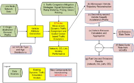
emissions estimation. The simulator framework can be visualized as Figure 2.1 has two different modules namely a traffic simulation module and an emissions estimation module. Data flow between these two modules should be consistent and uninterrupted in ideal conditions.
There have been many efforts in the past to couple an emission model with a traffic simulator either manually or directly. AIMSUN has been used with a European modal emissions model, VERSIT+ (Ligterink & Lange, 2009). MOBILE6 emissions model has been coupled with EMME/2 and PARAMICS (Bartin et al., 2007). MOVES emission model has been used with PARAMICS, DynusT, and VISSIM (Lin, Chiu, Vallamsundar, & Bai, 2011b; Song et al., 2012; Xie et al., 2011). Dynamic linkage of traffic and emissions models is challenging and can lead to significantly longer run times. Evaluation for a large-scale network is a trade-off between estimation accuracy and computational tractability. Therefore, it is a challenge to properly estimate emissions related impacts that is greatly exceeded by the imprecision and/or inaccuracy of the estimate.
Figure 2.1. Modules of integrated traffic simulation and emission estimation
typically use 0.1 seconds as the simulation interval. To ensure theoretical convergence of the integrated models, it is necessary to use multiple iterations between different
simulation/assignment components to determine the mobility and emission impact of high-level demand and traveler behaviors. However, internal discrepancies between different modeling resolutions make tight interconnections and consistent modeling extremely challenging.
2.1.6 Energy use and emissions estimation
Effective tools to estimate emissions for different scenarios are required to assess the effect of these strategies at different spatial and temporal resolution. There are several emissions models available that can estimate vehicle emissions for the prediction and management of air pollution levels near roadways. These models use information on weather, fuel type, fleet composition, vehicle type, and activity schedule as input.
For planning purposes, average speed and flow based models have been used for a long time. However, these models cannot adequately represent the dynamic effects of driving styles. Average speed based models use predetermined speed trajectories upon which
relationships between cycle or link-based average-speed and average emission rates are estimated (e.g. MOBILE (USEPA, 2007), EMFAC (CARB, 2002), COPERT (Ntziachristos et al., 2000)). US Environmental Protection Agency (EPA) have developed MOVES that can take into account a second-by-second vehicle speed trajectory (Chamberlin, Swanson,
Vehicle specific power (VSP) based estimation
VSP is a well-evaluated and widely used quantitative indicator of engine power demand that is an excellent predictor of vehicle fuel use and that is also highly correlated with vehicle tailpipe exhaust emissions for a wide range of pollutants (Jimenez-Palacios, 1998). VSP is a function of vehicle speed, road grade, and acceleration which accounts for kinetic energy, rolling resistance, aerodynamic drag, and gravity (Zhai, Frey, Rouphail, Goncalves, & Farias, 2009). It is usually reported as power required per mass of the vehicle (for example:
kilowatts per ton). Calculated VSP is categorized into different operating mode bins by speed and VSP ranges to estimate emissions factor for vehicles. Therefore, VSP is a parameter with important practical application. But accurate determination of VSP depends on proper
quantification of measured vehicle operating characteristics, such as speed, acceleration, road grade etc. Microscopic traffic characteristics e.g. speed, acceleration, headway etc. are highly dependent on the roadway, traffic, driver behavior characteristics.
VSP is usually estimated using developed equations for different classes of vehicles. According to MOVES the equation to calculate VSP is expressed as
𝑉𝑆𝑃 = (𝐴
𝑀) 𝑣 + ( 𝐵
𝑀) 𝑣2+ ( 𝐶
𝑀) 𝑣3+ (𝑎 + sin(𝛷))𝑣
Where: A, B and C refer to the rolling term, rotating term and the drag term respectively. M is the vehicle mass, is the vehicle speed, a is vehicle acceleration and Φ is road grade. The
parameters are different for each vehicle type.
MOVES provides default coefficients for different group of vehicles. Derivation of these coefficients is based on chassis dynamometer tests. The VSP formulation for light-weight vehicles provided by MOVES is
VSP = vehicle specific power, kW/ton
v= speed at time t, m/s ; a = acceleration at time t, m/s2 A= rolling resistance coefficient = 0.1565 kW-sec/m
B= rotational resistance coefficient = 2.002X10⁻³ kW-sec2/m2 C= aerodynamic drag coefficient = 4.926X10⁻⁴ kW-sec3/m3 m = vehicle mass = 1.479 ton.
EPA MOVES model
On March 2, 2010, USEPA announced the official release of the Motor Vehicle Emissions Simulator (MOVES2010) for use in state implementation plan (SIP) submissions to EPA and regional emission analysis for transportation conformity (Koupal, Cumberworth, Michaels, Beardsley, & Brzezinski, 2002). It replaced MOBILE 6.2 model where vehicle emissions rates represent averages over a driving schedule with defined average speed. MOVES2010 considers the relative time spent and emissions rate in vehicle speed and vehicle specific power bins (Fujita et al., 2012). Except for braking and idling, these OpMode bins are
stratified by 21 speed ranges (<25 mph, 25 to 50 mph, and >50 mph) and by Vehicle Specific Power (VSP) (Koupal, Michaels, Cumberworth, Bailey, & Brzezinski, 2002; Vallamsundar & Lin, 2011). The main purpose of this tool is to quantitatively predict emissions from mobile sources for a wide range of user-defined parameters e.g. vehicle type, time periods, geographical areas, pollutants, vehicle operating characteristics and road type (EPA, 2012). Therefore, MOVES is a significant improvement in the state-of-art for emissions estimation. The inputs from traffic simulation software can be linked to MOVES in three different formats:
b) Link driving schedule (LDS) for each link of the network. LDS is a time dependent speed profile for a particular link. Generally LDS is selected for a representative vehicle or by sampling.
c) Operating mode distribution of vehicles of the link.
However, MOVES is computationally intensive. Some investigators have attempted to use traffic simulation output for vehicle speed trajectories as input to MOVES, leading to time consuming computations for evaluation of different traffic management strategy scenarios.
Simplified emissions estimator – MOVESLite
As an alternative approach, a reduced form version of MOVES, referred to as MOVES Lite, has been recently developed (Frey & Liu, 2013). MOVES Lite is based on the same
computational structure as MOVES with respect to Op Mode bins and, therefore, is capable of estimating emissions for any specified speed trajectory. MOVES Lite is less
computational intensive than MOVES because it is calibrated to a base cycle and employs a cycle correction factor to adjust for differences in emission rates between any cycle of interest and the base cycle. MOVES Lite is based on a more limited set of vehicle types and pollutants than MOVES. Since traffic simulations are often for periods of a few hours, MOVES Lite does not take into account variations in factors such as fuel properties, inspection and maintenance programs, and ambient conditions that do not change
substantially or at all during such short periods of time. MOVES Lite is 3,000 times faster and can produce emissions estimates within ±5% deviation compared to MOVES.
weighted combinations of OpMode bins, a similar approach can be used as part of a simplified model that can be directly coded as part of a traffic simulation model.
MOVESLite harnesses these benefits to develop a less computationally intensive vehicle emission estimation module. The conceptual model of MOVESLite is based on (a) base emission rate for site-specific characteristics (b) a cycle correction factor for speed
trajectories and OpMode bin emission rates. The cycle correction factor is calculated using the following equation
CCFp,c,a,v= (
(∑m fmc × ERp,a,v,m)
(∑m fmb ×ERp,a,v,m)) ( Vb Vc) Where,
ERp,a,v,m = default emission rate for pollutant p, age a, vehicle type v, in operating
mode bin m, gram/hour
fm c = fraction of time in OpMode bin m in cycle c fm b = fraction of time in OpMode bin m for base cycle b Vc = cycle average speed for cycle c, mph
Vb = cycle average speed for base cycle b, mph
The base emissions rate is then corrected for the simulated cycle using the following equation
CEp,c= ∑ {[∑(EFp,b,a,v× CCFp,c,a,v× fa,v) a
] × fv} v
Where,
CE p,c, = cycle average emission factor for any arbitrary driving cycle c, for pollutant p, for a fleet of vehicles with mixed types and ages, gram/mi ER p,b,a,v = base emission rate for base cycle b, age a, vehicle type v, and pollutant
p, gram/mi
CCFp,c,a,v = cycle correction factor for driving cycle c, age a, vehicle type v, and pollutant p
c = cycle c b = base cycle p = pollutant
Comparison of the 2 models across similar criteria shown in Table 2.1 and Table 2.2.
Table 2.1. Performance of MOVES across different functional criteria
Criterion MOVES
Accuracy Accurate comparing with empirical emission factors.
Runtime Relatively slow.
Requirement for Input Substantial input data requirements.
Requirement for Platform Need to install MOVES package, JAVA, and MySQL. Connection with TDM and
TSM
Difficult to be coupled into TDM or TSM.
Usability Errors, warnings arise frequently, especially for beginning users.
Time consuming procedures
Adjust fuel property, temperature, humidity, air conditioning use, and I/M program for each link in the network.
Vehicle dynamic data Second by second data, or OpMode distribution
Vehicle Types 13 Vehicle types: Passenger Car, Passenger Truck, Refuse Truck, Single-Unit Short-Haul, Truck Single-Unit Long-Haul Truck, Motor Home, Intercity Bus, Transit Bus, School Bus, Combination Short-Haul Truck , Combination Long-Haul Truck, Motorcycle Adjusted emission rate map
(reflecting vehicle distribution and climate)
Table 2.2. Performance of MOVES lite across different performance criteria
Criterion MOVES lite
Accuracy Within ±5% errors comparing with MOVES.
Runtime 3000 times faster than MOVES.
Requirement for Input Limited input data requirements.
Requirement for Platform Can be run in MS EXCEL or MATLAB. It has a computational algorithm.
Connection with TDM and TSM
Can be integrated into TDM or TSM easily.
Usability User-friendly.
Time consuming procedures Set fuel property, temperature, humidity, air conditioning use, and I/M program constant by link in the network.
Vehicle dynamic data Same as MOVES
Vehicle Types For U.S. based model: Five vehicle types that comprise of more than 95% of the fleet: Passenger Cars, Passenger Trucks, Light Commercial Trucks, Single Unit Short Haul Trucks, and Combination Long Haul Trucks.
Adjusted emission rate map (reflecting vehicle
distribution and climate)
Yes, took vehicle distribution into account.
2.1.7 Characterization of TMS impacts on emissions
Modeling both supply- and demand-side TMS requires proper characterization and
Mode shift (MS) is a popular TDM technique that is intended to reduce the number of vehicle trips. MS involves combination of different mix of strategies to promote HOVs by improving HOV lanes, ridesharing and reducing single occupancy vehicles (SOV) through parking regulation and congestion pricing. A TDM program in an area wide level of
application can reduce vehicle miles traveled by 4%-8% (Meyer, 1999). Situations for which MS may be most effective include congested urban areas; a reduction of VMT is expected to improve traffic operations and consequently reduce emissions. However, for a relatively unsaturated network, MS is not expected to bring significant improvement and may even increase emissions.
suitable to assess emissions impacts of FR on a regional network. Even though a few previous studies assessed effects of vehicle turnover on emissions (Frey, Zhai, & Rouphail, 2009), comparable effectiveness of FR as a TMS was never assessed that can provide balanced insight regarding what combination of approaches may be effective in reducing emissions.
Cycle average emission rates when plotted against cycle average speed typically exhibit a parabolic shape, with high emissions rates at both ends and low emissions rates at moderate speeds of around 40 to 60 mph (Barth & Boriboonsomsin, 2009), depending on the pollutant. This relationship has motivated the consideration of congestion mitigation, speed management, and traffic smoothing strategies. Related TMS include variable speed limits, dynamic intelligent speed adaptation (ISA), congestion pricing, among others. Peak spreading (PS) is a traffic smoothing strategy is aimed at decreasing the frequency and intensity of acceleration and deceleration events due to congestion. PS can be achieved by altering the trip departure time choices of individuals by providing network congestion information. It can also increase network capacity significantly (Mahmassani & Liu, 1999). However, signs of PS implementation are only found in smaller cities where potential for urban sprawl and decentralization is much more limited (Gordon, Kumar, & Richardson, 1990).
reason, the majority of the previous literature was limited to a single corridor or a small or medium size network. However, advanced traveler information systems (ATIS) such as variable message sign (VMS) and radio broadcasts can have network wide influence on traveler choice, and thus can be used in response to incidents to encourage changes in trip departure time or diversions.
2.2 Research Questions
The two key research questions are addressed in this chapter – (1) how can emissions
impacts from a large-scale network be assessed? and (2) how do different TMS interventions on the network impact travel behavior, driving activity, and emissions at a regional and corridor level?
the emission model, which calculates the distribution of trip time in each VSP- and speed-based operating mode bin, calculates emissions speed-based on operating model bin emission rate tables (e.g., Table 2.3), and makes corrections based upon base cycle rates and vehicle attributes. In general, the procedure can be described in four steps; described in some detail next.
1) Vehicle Generation 2) Traffic Assignment
3) Vehicle Trajectory Reconstruction 4) Microscopic Emissions Estimation
Table 2.3. Selected Average Emission Rate for Zero-Age Passenger Cars (Frey, Yazdani-Boroujeni, Hu, Liu, & Jiao, 2013)
Operating Mode Energy (KJ/h) CO2 (g/h) NOX (g/h) CO (g/h) HC (g/h)
0 49206 3536 0.05 2.37 0.04
1 45521 3271 0.01 4.06 0.00
… … … …
Figure 2.2. Systems framework of DTALite and MOVES Lite
Step 1: Vehicle generation (with type and age distribution)
A typical traffic demand database describes the number of vehicles traveling between each origin and destination pair in the network, and the demand type associated with the vehicles, such as LOV (low occupancy passenger vehicle), HOV (high occupancy passenger vehicle) and trucks. Demand type classes are typically used to study different road tolling rules and different values of time in traffic demand management applications. The challenge is how to reasonably generate the detailed vehicle type and age distribution required for emission estimation. First, a table similar to Table 2.4 is used to distribute vehicles in each demand type to different vehicle types. Then a table similar to Table 2.5 is used to further
disaggregate vehicles in each vehicle type to different age groups based on a simple
calibrated using state-wide or local regional data sources (Bureau of Transportation Statistics, 2013).
Table 2.4. Example Sample Distribution for Mapping from Demand Type to Vehicle Type
Demand Type Vehicle Type Passenger Car Passenger Truck Light Commercial Truck Single Unit Short-haul Truck Combination Long-haul Truck Single occupancy passenger vehicle (SOV)
80% 20% 0% 0% 0%
High occupancy passenger vehicle (HOV)
80% 20% 0% 0% 0%
Truck 0% 0% 72% 22% 6%
Table 2.5. Vehicle Age Distribution by Type and Age (Frey et al., 2013)
Vehicle
Type Name
Vehicle Age Distribution
Age 0 Age 5 Age 10 Age 15
1 Passenger Car 6% 48% 28% 18%
2 Passenger Truck 3% 43% 26% 28%
3 Light Commercial Truck 3% 44% 26% 27%
4 Single Unit Short-haul Truck 4% 52% 23% 21%
5 Combination Long-haul Truck 4% 52% 23% 21%
Based on the number of vehicles traveling from each origin to each destination, the departure time profile, and the mapping information from demand type to vehicle type and age
Step 2: Traffic assignment and simulation modules to achieve user equilibrium Using network data, generated vehicles, and traffic control measures, the mesoscopic DTA model typically performs the following steps at each iteration.
a. Shortest Path Calculation: Calculates the time-dependent least-cost or least-time path for each vehicle based on its origin, destination and departure time.
b. Traffic Simulation: Perform traffic simulation to move the vehicles from their origins to their destinations, subject to link and node capacity constraints. Update the time-dependent link travel times for next shortest path calculation.
c. Vehicular Flow Assignment: The assignment module assigns a certain percentage of vehicles to newly-computed least-cost or least-time path.
d. Convergence Checking: The assignment and simulation steps are repeated until the equilibrium is achieved. Typically, 20-40 iterations are required to reach a desirable relative user equilibrium gap value (e.g., 1%).
DTALite is a simulation-based dynamic network loading model used to move vehicles through the network. Based on a triangular flow-density relation shown in Figure 2.1, there are two closely related finite-difference-based numerical solution schemes to solve the traffic simulation problem as the first order kinematic wave problem: (i) Newell's
simplified model (Newell, 1993) that keeps track of shock wave and queue propagation using cumulative flow counts on links, and (ii) Daganzo’s cell transmission model (Daganzo, 2006) that adopts a “supply-demand” or “sending-receiving” framework to model flow dynamics between discretized cells. Newell’s kinematic wave (KW) model is used in DTALite’s
Bounda ry of sh
ock wa ve
back w
ard w ave Time now t
S p a ce a x is BWTT Link Length D(l,t-BWTT)
A(l,t) k
jam(
l)×
len gth(
l)×n
lanes (l)
t d t d t d
j-4 j-3 j-2 j-1 j d t
X(j-4, t-BWTT)
X(j,t)
Cumulative flow count N(x,t) space
Space-time vehicle trajectory X(j,t) space
Time
Link Length
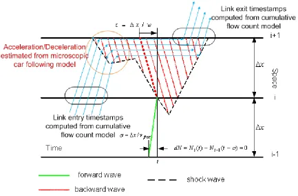
Figure 2.3. Consistent representation of backward wave propagation in both Newell’s kinematic wave and simplified linear car following models (Zhou et al., 2015) By explicitly using the cumulative arrival and departure curves, Newell’s flow model
provides an effective means to realistically represent traffic dynamics and capture (forward and backward) shockwaves as the result of bottleneck capacities. In addition, compared to other cell-based models that need to subdivide a long link into segments with short lengths, Newell’s model can handle reasonably long links with homogeneous road capacity. Its
simple traffic flow model and computational efficiency make it particularly appealing in establishing theoretically sound and practically operational DTA models for large-scale networks. There are a number of related studies on Newell’s kinematic model, to name a few,
DTALite adopted Hurdle and Son’s framework (Hurdle & Son, 2000) to illustrate how Newell’s approach can model backward waves using cumulative flow counts. Let x
denote the location along the corridor. A wave w(q, x) represents the propagation of a change in flow q and density k along the roadway,
𝑤(𝑞, 𝑥) =𝑑𝑥𝑑𝑡. (1)
Let us focus on the change of N curves along a characteristic line (wave) at links; that is,
𝑑𝑁(𝑥, 𝑡) =𝜕𝑁𝜕𝑥𝑑𝑥 +𝜕𝑁𝜕𝑡𝑑𝑡 = 𝑞𝑑𝑡 − 𝑘𝑑𝑥 (2)
where N(x, t) is the actual cumulative count of vehicles that pass location x from time 0 to
time t. Along the movement of a wave, the definition of w in equation (1) leads to 𝑑𝑡 = 𝑑𝑥𝑤 and simplifies equation (2) as
𝑑𝑁(𝑥, 𝑡) = 𝑞𝑑𝑡 − 𝑘𝑑𝑥 = (−𝑘 +𝑞𝑣) 𝑑𝑥. (3)
In the triangular-shaped flow-density relation, the values of (forward and backward) waves are constant. In the case of backward wave propagation, the congested region of the
triangular shaped flow-density model gives −𝑘 + 𝑞
𝑤𝑏= −𝑘𝑗𝑎𝑚 . (4)
Step 3: Vehicle trajectory construction module
DTALite outputs the link arrival and departure times for each vehicle, which can be used to construct cumulative vehicle arrival and departure counts on each link. Given the arrival and departure time of the individual vehicle on a link, we adapt Newell’s simplified linear car
following (LCF) (Newell, 2002) model to reconstruct the vehicle trajectory in the link. Then the detailed second-by-second vehicle speed and acceleration are derived from the
reconstructed vehicle trajectory. It is not necessary to construct the vehicle trajectory for each iteration of the DTA simulation. To save computational time, one can convert only the cumulative flow counts from the last iteration of the DTA process to generate second-by-second speed profiles and corresponding emission results.
The main idea of Newell’s car following model is that a (following) vehicle n maintains a
Figure 2.4. Constructing microscopic vehicle trajectory from mesoscopic simulation results (Zhou et al., 2015)
Mathematically, Newell’s car following model states that the vehicle trajectory relationship
between the following vehicle n and the lead vehicle n-1 is defined as:
1
n n n n
x t
t
x t d(6)
where xn1
t is the position of the lead vehicle at time t, x tn
t
n
is the position of thefollowing vehicle at time
t
t
n;t
n andd
n are the appropriate time and space gaps,respectively. Given the vehicles’ arrival and departure times on the link from a macroscopic
dynamic traffic assignment and simulation model such as DTALite, the procedure for calculating the vehicle trajectories along this link is described below.
f
v
: the free flow speed on the link;d: the minimum space gap;
t
: the minimum time gap;( )
Arr n : the arrival time of vehicle n at the upstream node of the link;
( )
Dep n : the departure time of vehicle n at the downstream node of the link;
T
: the time step increment (e.g. 0.1 seconds);
Variables:
,X n t : the position of vehicle n at time t;
For each vehicle n1,K,N
Initialize the starting position of a link X n Arrival n
, ( )
=0;For each time interval t = Arr n( ) to Dep n( )
Calculate free-flow driving position:
,
min
, ,
F
f
X n t T X n t v T L
; If n is the first vehicle, where n0
,
F
,
X n t T X n t T
Else
Calculate position determined by backward wave propagation from the leader n-1:
,
1,
B
X n t T X n t T
t
d; Calculate the final feasible position:
,
min
F
,
, B
,
X n t T X n t T X n t T
End If t t T;
End For End For
A recent paper by Dr. Daganzo in UC Berkeley (Daganzo, 2006) has shown that, by assuming a triangular flow-density diagram, vehicle trajectories constructed from a
simplified kinematic wave model are equivalent to those generated by Newell’s simple linear car-following model and two types of cellular automata (CA) models within a certain
approximation range. In a calibration and validation study for a number of well-known car following models, Newell’s simplified LCF model showed reasonable performance with
limited calibration efforts.
Step 4: Microscopic emissions module
MOVES Lite first calculates the second-by-second VSPs based on the corresponding vehicle operating parameters. Using a combination of calculated VSPs and the vehicle speed, the calculation process then finds the appropriate operating modes from the operating mode bin table (e.g., Table 2.3). This is followed by another table lookup (Table 2.4, Table 2.5) with the vehicle emission rate table based on operating mode, vehicle type and age. The emission and fuel consumption are accumulated and corrected with base cycle emission rates
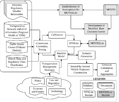
2.4 Methodology for Evaluation of Transportation Management Strategies (TMS) The integration of MOVES Lite with mesoscopic simulator DTALite in a multi-resolution platform provided a unique opportunity to assess emissions impacts of network interventions in a consistent and efficient manner (Frey & Liu, 2013). The methodology discussed in this chapter attempts to organize these different components as a system framework, depicted in Figure 2.5. The system relies on two parallel processes: attribution of emissions estimation module, MOVES Lite (shown in grey boxes) and functioning of DTALite in simulation of TMS scenarios. The left box in Figure 2.5 shows the input requirements for the framework. MOVES Lite depends on site-specific vehicular, regulatory, and weather information to establish assumptions regarding simplification of MOVES database. Network and traffic related input data are converted, corrected and verified to assemble the baseline network. Proper characterization of TMS is supported through regulatory, policy, economic, and technological evaluation of these interventions (shown in clouds at the bottom). TMS’s can
then be implemented in the calibrated baseline model and the estimation of emissions can be done through the integrated DTALite-MOVES Lite interface.
2.4.1 Data preparation
Preparation of network data
major road segments (example: Traffic.com, INRIX). Supplementary data sources could include video surveillance and floating car sensing information.
Figure 2.5. System framework and data-flow for assessing emissions impacts of Transportation Management Strategies
Preparation of emissions data
and OpMode, and vehicle type and age distribution. Agent based DTALite stores type and age characteristics of each vehicles and serves as the reverse interface. Trajectories are generated in terms of 1 Hz speed and acceleration for each modeled vehicle. The trajectories are used to calculate vehicle specific power (VSP) and the fraction of time spent in each OpMode for a given cycle. Therefore, a cycle correction factor (CCF) for link based driving cycle can be generated for each vehicle type. The base cycle emission factors can then be corrected and aggregated over a link for each vehicle type to produce the desired link emissions estimates. Thus, the spatial resolution of the estimate is the link. However, the estimation of emissions will depend on a proper characterization of speed trajectory in DTALite. For validation purposes, the LCF generated trajectories are compared to real world measurement of driving activity. The result have shown some unrealistic acceleration and deceleration events, and a lack of diversity between simulated trajectories. A potential remedy to this problem is to separate the cycle profile in segments and match them with real-world micro-trips; matched profile segments that can then be combined to reconstruct the vehicle trajectory (Zhou et al., 2015). In spite of this model limitation, the method provided a practical way to bridge data requirements between a mesoscopic traffic model and
microscopic emissions estimation model.
2.4.2 Experimental design for evaluation of TMS
Preparation of baseline network
The baseline network represents characteristics and conditions of the present ‘without
intervention’ scenario. It is essential that the baseline model emulate field observed volumes,