DOI: 10.1534/genetics.109.107391
The Accuracy of Genomic Selection in Norwegian Red Cattle Assessed
by Cross-Validation
Tu Luan,*
,1John A. Woolliams,*
,†Sigbjørn Lien,
‡Matthew Kent,*
,‡Morten Svendsen
§and Theo H. E. Meuwissen*
*Department of Animal and Aquacultural Sciences and‡Centre for Integrative Genetics, Norwegian University of Life Sciences, N-1432 A˚ s, Norway,†The Roslin Institute (Edinburgh), Royal (Dick) School of Veterinary Studies, University of Edinburgh,
Roslin, Midlothian EH25 9PS, United Kingdom and§Geno Breeding and Artificial Insemination Association, 1432 A˚ s, Norway
Manuscript received July 15, 2009 Accepted for publication August 12, 2009
ABSTRACT
Genomic Selection (GS) is a newly developed tool for the estimation of breeding values for quantitative traits through the use of dense markers covering the whole genome. For a successful application of GS, accuracy of the prediction of genomewide breeding value (GW-EBV) is a key issue to consider. Here we investigated the accuracy and possible bias of GW-EBV prediction, using real bovine SNP genotyping (18,991 SNPs) and phenotypic data of 500 Norwegian Red bulls. The study was performed on milk yield, fat yield, protein yield, first lactation mastitis traits, and calving ease. Three methods, best linear unbiased prediction (G-BLUP), Bayesian statistics (BayesB), and a mixture model approach (MIXTURE), were used to estimate marker effects, and their accuracy and bias were estimated by using cross-validation. The accuracies of the GW-EBV prediction were found to vary widely between 0.12 and 0.62. G-BLUP gave overall the highest accuracy. We observed a strong relationship between the accuracy of the prediction and the heritability of the trait. GW-EBV prediction for production traits with high heritability achieved higher accuracy and also lower bias than health traits with low heritability. To achieve a similar accuracy for the health traits probably more records will be needed.
G
ENOMIC selection (GS) is a new technology that is expected to revolutionize animal breeding. It is distinct from traditional selection methods where phenotype and pedigree information is combined to predict breeding values and where at least one source is necessary for a prediction. Estimation of GS breeding value is based on the estimation of marker effects cover-ing the whole genome and combines these estimates with the marker genotypes to obtain breeding value estimates. Given a sufficiently dense genomewide marker map, all the genetic variance is expected to be ex-plained by the markers, and all quantitative trait loci (QTL) are in linkage disequilibrium (LD) with at least one marker (Caluset al.2008). This allows GS topre-dict genomewide estimates of breeding values (GW-EBV) without the need of phenotyping the selection candidates. A potential cost reduction of up to 90% can be achieved for a breeding program by GS (Schaeffer
2006), because only a moderate number of individuals are required to have both known marker genotypes and phenotypes. These individuals form a reference data set for the estimation of GW-EBV. The knowledge obtained from the reference data set can be applied to the
calculation of GW-EBV for the selection candidates on the basis of their marker genotypes, with an accuracy that is found in the validation of the prediction (Goddardand Hayes2007).
For a successful application of GS, based on a ref-erence data set, to a usually much larger population of selection candidates without phenotypic records, accuracy of the prediction is a key issue to consider (Goddard and Hayes 2009). Since GS was first
pro-posed by Meuwissenet al.(2001), many research works
using simulated data have been performed on this issue (Calusand Veerkamp2007; Habier et al.2007;
Kolbehdariet al.2007; Caluset al.2008; Solberget al.
2008). The recent availability of genomewide dense SNP marker maps has made GS with real data feasible. Studies of the accuracy of genomic predictions have emerged in some animal species, including mice (Lee et al.2008; Legarraet al.2008), chickens (Gonzalez
-Recioet al.2009), and cattle (Hayeset al.2009), and in
plant species [for example, barley (Zhonget al.2009)].
For GS applied to dairy cattle, accuracies for the GW-EBV have been reported in North American Holstein (VanRaden et al. 2009), Australian Holstein–Friesian
(Hayeset al.2009), and New Zealand Holstein–Friesian
and Jersey dairy cattle (Harriset al.2008).
In the present work we applied GS to Norwegian Red dairy cattle to investigate the accuracy and possible bias
1Corresponding author:Department of Animal and Aquacultural
Scien-ces, Norwegian University of Life ScienScien-ces, Box 5003, N-1432 A˚ s, Norway. E-mail: tu.luan@umb.no
of GW-EBV prediction for the phenotypes of milk production, clinical mastitis, and calving ease, by using real bovine genotyping data. Three methods, best linear unbiased prediction, Bayesian statistics, and a mixture model approach were used in the study, and their accuracies and biases of the GW-EBV were compared. To estimate the accuracy and bias of the GW-EBV the approach of cross-validation was employed, making use of estimates of breeding value from the Norwegian Red dairy cattle breeding scheme.
MATERIALS AND METHODS
Genotypic and phenotypic data:There were 500 Norwegian Red bulls selected for this study with 466 sons of 34 sires, with no son also being a sire. Sons had been progeny tested between 2001 and 2006, and sires tested before 2001. The numbers of sons chosen for years 2006, 2005, 2004, 2003, 2002, and 2001 are 36, 44, 98, 98, 100, and 90, respectively. All sons and sires were genotyped at CIGENE (www.cigene.no), using the 25K MIP-SNP chip array from Affymetrix (San Diego). All data from an individual SNP were deleted if (a) pedigree information exposed .2.5% non-Mendelian sire–offspring inheritance patterns, (b) its genotype probabilities signifi-cantly deviated from the Hardy–Weinberg proportions (P, 0.01%), (c) across samples.25% genotypes were missing, or (d) its minor allele frequency (MAF),2.5%. A total of 18,991 SNPs remained after filtering. The phenotypic data of all 500 bulls used for the study are daughter-yield deviations (DYDs) (Wigganset al.1992) for the traits: metric tons of milk yield,
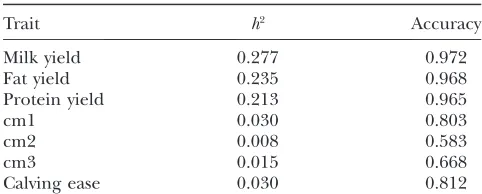
kilograms of milk fat yield, kilograms of milk protein yield, calving ease, and clinical mastitis (cm). Clinical mastitis was considered in three traits defined by period of first lactation: cm1, 15–30 days in milk; cm2, 31–120 days in milk; and cm3, 121–305 days in milk. The data were based on the average of 1038 daughters, varying from 111 to 21,391, and were available for all bulls for all traits. Accuracy of DYD for a trait is defined as the average of the accuracies of the DYDs of 500 bulls for the trait and was obtained together with DYD from BoviBank Ltd. (www.bovibank.no). The accuracies of DYDs are listed in Table 1. The genotype data and phenotype data of all 500 bulls constitute the complete data used in the present work.
Training data: The training data sets were each obtained by masking the phenotype,i.e., setting the phenotype ‘‘un-known,’’ for a defined number of individuals. The individuals whose phenotype was masked were selected in two different ways. The first way was through random selection: here 100 individuals at a time were randomly selected, without re-placement, to produce five nonoverlapping training data sets; i.e., every phenotype was masked precisely once in the training data sets. In this article this way is referred to as ‘‘20% random masking.’’ The second way was to select individuals on the basis of their year of progeny testing: seven training data sets were obtained for years 2006, 2005, 2004, 2003, 2002, 2001, and before 2001. The number of phenotype-masked individuals in a training data set for a year of testing is the number of bulls selected for this year. We called this way of selection ‘‘cohort masking.’’ The nonmasked data were analyzed by the models described in the ‘‘data analysis’’ section to predict the masked phenotypes. This resulted in each bull having a predicted phenotype from each masking method and this was compared to the realized DYD. The correlation coefficient between the predicted and realized DYDs was calculated and used as a measure of the accuracy of the GW-EBV predictions.
Additional training sets for production traits were gener-ated to test the impact of increasing the random masking to
50% by randomly allocating each individual to one of two training sets. This implies that there were only 250 individuals with phenotypes in the training data set, instead of 400 as in 20% random masking. To obtain standard errors, for both 20% and 50% random masking the division into sets and all the subsequent analyses described in theData analysissection were replicated six times.
Data analysis: Three models were used to estimate the marker effects: best linear unbiased prediction (G-BLUP), Bayesian statistics (BayesB), and MIXTURE. G-BLUP esti-mates the effects of the markers by best linear unbiased prediction (Henderson1975), assuming that every marker
explains an equal proportion of the total genetic variance. BayesB is described in detail by Meuwissenet al.(2001) and
estimates the variance explained by every marker, using a prior distribution that assumes that this variance is small, denoted as s2, with probability (1g
B);i.e., the marker has virtually no effect or comes from an inverse-chi-square distribution with probabilitygB. The probabilitygB represents the probability that a marker has a substantial effect and was varied in the data analysis since it is generally unknown. Meuwissen et al. assumeds2¼0 for markers with small estimated effects, but
by havings2slightly larger than zero, the model can be
im-plemented as a Gibbs sampling algorithm, which has compu-tational advantages. Here, the small variances2was estimated
from the data,i.e., from the genes with small effect. In the Gibbs chains2was sampled from the conditional posterior,
which is SSaxn22, where x 2
n2 is a random deviate from the inverse-chi-square distribution withn2 d.f.;nis the number of SNPs with small effect in the current iteration of the chain; SSa¼SIiai2, whereIiis an indicator variable taking values 1 if
SNPi belongs to the SNPs with small effects in the current
iteration andIi¼0 otherwise; andaiis the current solution of
the effect of SNPi. As mentioned above, if SNPs were assumed
to have substantial effect, they had an individual variance estimated. If this individual variance was,s2, the SNP effect
was removed from the set of SNPs with substantial effect, to ensure that the substantial effect SNPs always had higher variance than the small effect SNPs. This is similar to including a polygenic term in the BayesB model (Calusand Veerkamp
2007; Solberget al.2008), but where the correlation matrix of
the polygenic effects is defined by the markers with small effect instead of by the pedigree.
Since BayesB makes quite strong assumptions about the prior distribution of the marker effects, which may not be true in real data, we also used a model that attempts to estimate this prior distribution. For the latter, we made use of a property of mixtures of normal distributions, namely that they can be used to approximate any other (prior) distribution (Silverman
1996). In the MIXTURE model we assumed that the marker effects came from a mixture of two distributions: one distribu-tion with large variance (accommodating large marker effects) and one with small variance (accommodating small marker
TABLE 1
Heritability and accuracy of DYD for studied traits
Trait h2 Accuracy
Milk yield 0.277 0.972
Fat yield 0.235 0.968
Protein yield 0.213 0.965
cm1 0.030 0.803
cm2 0.008 0.583
cm3 0.015 0.668
effects). This model was also implemented in a Gibbs sampling algorithm as described by George and McCulloch (1996)
except that the variance of the small SNP effects is estimated here. The distribution to which the marker belongs is sampled from the Bernoulli distribution, with parametergM. The pa-rameter gM, which reflects the proportion of the markers belonging to the large and the small variance distribution, is sampled using a noninformative Beta distribution as a prior. The variances of the two distributions underlying the mixture (s12ands22) are estimated using a noninformative chi-square distribution (SorensonandGianola2007).
The model of analysis that was used by G-BLUP, BayesB, and MIXTURE was
y¼m1X Nm
j¼1
Xjaj1e;
whereyis aN 31 vector of phenotypes (DYDs);Nmis the number of markers fitted;ajis the effect of the marker;Xjis a N 3 1 vector denoting the genotype of the individuals for markerj, withXij¼0 if individualiis homozygous for the first
allele at locusj, Xij ¼1=
ffiffiffiffiffiffi Hj
p
if heterozygous, Xij ¼2=
ffiffiffiffiffiffi Hj
p if individualiis homozygous for the second allele at locusj, and Xij ¼2qj=
ffiffiffiffiffiffi Hj
p
if the marker genotype is missing, whereqjis the
frequency of the second marker allele andHjis the marker
heterozygosity. The division by ffiffiffiffiffiffiHj
p
standardizes the variance of the marker genotype data to 1. The variance ofajis assumed
to be Vs/Nm for G-BLUP, is estimated by BayesB, and in MIXTURE equalss12ors
2
2, depending on whether the marker
effect is small or large ands12ands
2
2are both estimated. Since
the traits are DYDs,Vsis the sire variance, which is one-quarter of the total genetic variance, and was obtained from Interbull (http://www-interbull.slu.se) together with the trait heritabil-ities (Table 1). Given the estimates of the marker effects and the marker genotypes, genetic values for the masked individ-uals are predicted as
GW-EBVi¼
XNm
j¼1 Xijaˆj;
whereXijis the marker genotype of individualifor markerj
coded the same as above, andaˆj is the estimated effect of
markerj. By adding the overall mean,m, to the GW-EBVi, and
assuming that the residual effect of the DYDs is on average 0, a predicted phenotype was obtained for every bull (whose phe-notype was masked). Since every bull’s phephe-notype was masked once in one of the training sets, a total of 500 predicted phenotypes were obtained for each model for a trait for a masking strategy. The correlation coefficient between the predicted and realized phenotypes was calculated and used as a measure of the accuracy of the GW-EBV predictions. The regression of the realized phenotypes on the predicted phenotypes is used as a measure of the bias of the GW-EBV, where a regression coefficient of 1 denotes no bias,,1 implies that extreme high (low) values of the GW-EBV over- (under)-predict the realized phenotypes, and vice versa for a regression coefficient.1. These summary statistics were examined both overall and within each masked set.
For BayesB calculation, the length of the Gibbs chain was 15,000 iterations and 5000 iterations were used for burn-in. For MIXTURE, the chain length was 12,000 iterations and burn-in was 8000 iterations. To ensure the convergence of the Gibbs chains used for BayesB and MIXTURE, 10 distinct chains were run for milk yield and the estimated accuracy was calculated from pooling the chains. It was found that the estimated accuracy did not change to three significant numbers after pooling 3 chains. This finding was tested for
other production traits and health traits. Consequently all results presented for Gibbs analyses are the average of 3 distinct Gibbs chains.
RESULTS
Determination of the number of markers with effects:The number of markers with a substantial effect in BayesB calculation determines the probabilitygBof a marker with substantial effect. In this study, this number is defined separately for different ways of masking data for each trait, by a set of BayesB calculations with dif-ferent numbers of effective genes. For example, for the random masking data for milk yield, we applied BayesB to the data with the number of effective genes 800, 1600, 2400, 3200, 6400, 9600, and 12,800, respectively.
The result in Figure 1 shows that the accuracy for GW-EBV prediction was affected little by the number of markers with an effect. Accuracies varied from 0.56 to 0.58 with respect to numbers of effective genes used. The maximum accuracy achieved for random masking in Figure 1 suggests that 3200 was approximately opti-mal, and thus gB¼0.169 (3200/18,991) was used for milk yield. ThegBvalue for milk yield for cohort mask-ing of data was determined similarly, and the lower value ofgB¼0.126 was found to be slightly better than other values of gB. For other production traits and health traits, the same approach was applied to setgB, and the values are shown in Table 2. Table 2 also listsgMvalues for MIXTURE, together withs12ands22as the variances of the two distributions underlying the model. In con-trast to BayesB, optimal numbers of effective genes can be determined during the MIXTURE calculations, and Table 2 shows that thegMvalue for MIXTURE is mostly lower than thegBfor BayesB.
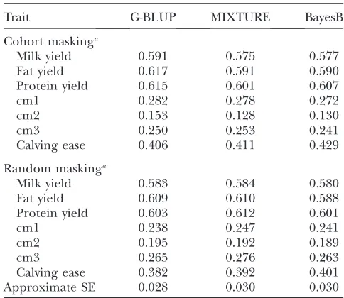
Accuracy of GW-EBV prediction: Table 3 shows the
accuracy of the GW-EBV prediction by the BayesB, MIXTURE, and G-BLUP methods. For 20% random masking, Table 3 shows the mean predictive accuracy
Figure 1.—Accuracy of GW-EBV prediction with the
obtained for predicting the 100 individuals in the validation set for analysis of the 400 in the training set. The mean is therefore an average of 30 values, 5 from each random division of the bulls into 5 sets of 100, and then replicated six times. The standard error is based on the variance between the replicate means. However, for cohort masking, the accuracy is combined using the single GW-EBV obtained for each of the 500 bulls. It is shown in Table 4 that in cohort masking, accuracies vary within a considerable range for offspring subsets with different population size and year of progeny test. For most traits, the prediction of the masked sire cohort using phenotypes of their offspring cohorts achieved higher accuracy than those of masked cohort offspring.
The general conclusion from Table 3 is that for the traits studied the differences between the methods are small, and are small compared to their standard errors. For random masking, all three methods used give sim-ilar mean accuracy and standard error. There is a trend among the methods for G-BLUP to have a higher accuracy than other methods for cohort masking. Among the three production traits the accuracy for milk yield is in general lower than that for fat yield and for protein yield, but again the difference between the accuracies is within the range of the standard error.
For health traits, Table 3 shows that the accuracies of GW-EBV are considerably lower than the accuracies for production traits. In addition, compared to the pro-duction traits, the health traits show bigger differences between mean accuracy and combined accuracy. This can be seen in Table 3 by the difference between mean accuracy and combined accuracy for cm1 and cm2, which is beyond the range of standard error of the accuracy.
Table 5 presents overall average accuracy and bias based on mean accuracies and biases for six replicates of 50% and 20% masking. Results in Table 5 show that accuracy for 20% masking with 400 phenotypes in the
TABLE 2
Estimates ofgBfor BayesB andgM,s12, ands22for MIXTURE for random masking and cohort masking
Trait
Random masking: Cohort masking:
BayesB MIXTURE BayesB MIXTURE
gB gM s12 s
2
2 g
B gM s12 s22
Milk yield 0.169 0.038 1.83106 4.03104 0.126 0.028 2.23106 9.13104
Fat yield 0.169 0.041 3.03103 1.63101 0.506 0.031 3.03103 2.23101
Protein yield 0.042 0.042 1.03103 7.93102 0.042 0.061 1.03103 6.03102
cm1 0.042 0.062 1.03108 4.53105 0.084 0.017 9.83109 5.03105
cm2 0.758 0.081 1.43109 3.03105 0.758 0.061 1.43109 2.03105
cm3 0.042 0.022 5.03109 1.33104 0.042 0.049 4.53109 1.13104
Calving ease 0.084 0.057 4.03108 1.23104 0.126 0.039 3.73108 1.33104
TABLE 3
Accuracy of GW-EBVs obtained by G-BLUP, MIXTURE, and BayesB
Trait G-BLUP MIXTURE BayesB
Cohort maskinga
Milk yield 0.591 0.575 0.577
Fat yield 0.617 0.591 0.590
Protein yield 0.615 0.601 0.607
cm1 0.282 0.278 0.272
cm2 0.153 0.128 0.130
cm3 0.250 0.253 0.241
Calving ease 0.406 0.411 0.429
Random maskinga
Milk yield 0.583 0.584 0.580
Fat yield 0.609 0.610 0.588
Protein yield 0.603 0.612 0.601
cm1 0.238 0.247 0.241
cm2 0.195 0.192 0.189
cm3 0.265 0.276 0.263
Calving ease 0.382 0.392 0.401
Approximate SE 0.028 0.030 0.030
a
The accuracy for cohort masking is shown as a combined accuracy estimated for 500 selected individuals, while the ac-curacy for random masking is shown as the mean of the accu-racies for five training data sets and the pooled approximate standard error.
TABLE 4
Mean, minimum, and maximum accuracies for six offspring training subsets and accuracy for sire data set in GW-EBV
prediction for cohort masking with BayesB
Offspring
Trait Mean Min Max Sire
Milk yield 0.501 0.295 0.659 0.735
Fat yield 0.574 0.272 0.688 0.778
Protein yield 0.482 0.252 0.654 0.718
cm1 0.271 0.163 0.349 0.426
cm2 0.109 0.033 0.307 0.012
cm3 0.251 0.140 0.311 0.525
training data set is significantly higher compared to 50% masking with 250 phenotypes in the training data set.
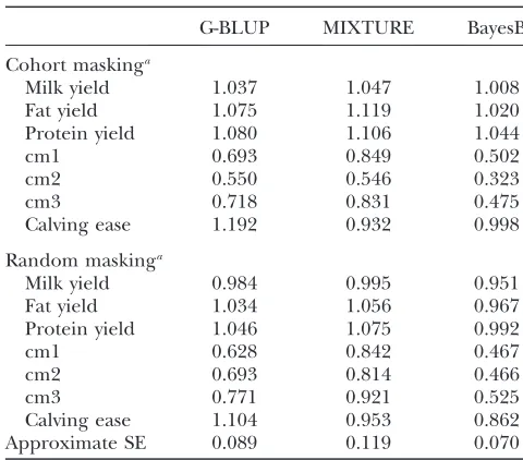
Bias of GW-EBV prediction:The degree of bias from
the methods is judged by comparing the regression co-efficients of phenotypes on predicted phenotypes with the value 1. Table 6 presents the bias of the GW-EBV prediction for the traits studied. As for the presentation of accuracy, for random masking, Table 6 shows the overall mean and the standard error of the bias of the predictions for six replicates of five training data sets, while for cohort masking, it is the combined bias esti-mated for all 500 selected individuals. The results show that for production traits the GW-EBV predictions for random masking had a lower bias compared to those for cohort masking, but these differences were within the standard errors. It is observed for the three mastitis traits in Table 6 that there is less bias if the prediction is more accurate. For example, for cm1, Table 3 shows the combined accuracy of the prediction for cohort masking is higher than the mean accuracy for random masking, and Table 6 shows the combined bias of cohort mask-ing is lower than the mean bias for random maskmask-ing. Among the four health traits, GW-EBV prediction for calving ease has the highest accuracy (Table 3), and the prediction is in general least biased (Table 6).
Accuracy and bias for a subset of markers: To
in-vestigate the effect of the number of markers fitted on the accuracy of the GW-EBV, for production traits, we randomly removed markers in the complete data sets and repeated the analyses described in materials and methods. In this work, 25, 50, and 75% of 18,991
markers were randomly selected and removed. This process was replicated six times to obtain standard errors
and results for cohort masking are shown in Tables 7 and 8. In general the results for the reduced marker data sets show similar features to those for the complete data with respect to the different traits, methods of analysis, and masking of the phenotypes. As expected, the accuracy of the prediction reduces as the number of markers becomes smaller. However, the decrease of the accuracy was small. For example, for G-BLUP applied to the three production traits, the combined accuracies of the GW-EBV decrease,9% of their original value for the subset with 75% of the markers removed.
DISCUSSION
This study applied genomic selection to real rather than simulated phenotypes in a setting in which it would be used in practice and where the predictive accuracy can be assessed by comparison with relatively precise estimates of breeding values obtained from phenotypic measurements and genetic evaluation using pedigrees. The existence of a relatively precise comparison allowed this study to compare the effectiveness of the different methods that might be employed. A total of519,000 measurements were made on individual dairy cows, to obtain the 500 DYD phenotypes on individual bulls used in the analysis. The GW-EBVs for individual bulls were calculated from the estimates of effects of 19,000 SNP markers alone and the accuracy of the estimates was determined by the correlation between predicted and realized DYDs,rDYD,GW-EBV. The estimates of the marker TABLE 5
Accuracy and bias of GW-EBV prediction for random masking with 250 DYDs and 400 DYDs in the training data set
Overall mean accuracya
Overall mean biasa
Trait 250 DYDs 400 DYDs 250 DYDs 400 DYDs
G-BLUP
Milk yield 0.547 0.599 1.010 1.022
Fat yield 0.569 0.611 0.999 1.033
Protein yield 0.550 0.594 1.006 1.035
MIXTURE
Milk yield 0.542 0.595 1.018 1.026
Fat yield 0.564 0.610 1.001 1.051
Protein yield 0.545 0.594 1.004 1.037
BayesB
Milk yield 0.538 0.585 0.957 0.967
Fat yield 0.552 0.590 0.927 0.970
Protein yield 0.546 0.589 0.954 0.973
Approximate SE 0.011 0.005 0.020 0.010
aThe accuracy and bias are shown as the overall mean
ac-curacies and biases for five training data sets and six replicates and the pooled approximate standard error.
TABLE 6
Bias of GW-EBVs obtained by G-BLUP, MIXTURE, and BayesB
G-BLUP MIXTURE BayesB
Cohort maskinga
Milk yield 1.037 1.047 1.008
Fat yield 1.075 1.119 1.020
Protein yield 1.080 1.106 1.044
cm1 0.693 0.849 0.502
cm2 0.550 0.546 0.323
cm3 0.718 0.831 0.475
Calving ease 1.192 0.932 0.998
Random maskinga
Milk yield 0.984 0.995 0.951
Fat yield 1.034 1.056 0.967
Protein yield 1.046 1.075 0.992
cm1 0.628 0.842 0.467
cm2 0.693 0.814 0.466
cm3 0.771 0.921 0.525
Calving ease 1.104 0.953 0.862
Approximate SE 0.089 0.119 0.070
a
effects came from training data sets and rDYD,GW-EBV derived from using cross-validation.
Generally, the estimated accuracies will underpredict the observed accuracy of selection,i.e., the correlation between GW-EBV and true breeding values,rGW-EBV,TBV, because the realized DYDs are not perfectly predicting the true breeding values. The expected correlations between the DYDs and genetic value,rDYD,TBV, are given in Table 9. A better estimate of the accuracy of the
GW-EBV (rGW-EBV,TBV) may be obtained by calculating
rDYD,GW-EBV/rDYD,TBV, whererDYD,TBVequals the accuracy of DYD (Table 1). In Table 1, there is a strong relation-ship between heritability and the accuracy of DYD,i.e.,
rGW-EBV,TBV. This suggests that data sets of .500 bulls are needed to achieve comparable accuracies for the less heritable traits, i.e., the health traits as shown by Daetwyleret al.(2008).
The G-BLUP method gave overall the highestrDYD,GW-EBV and little bias of the GW-EBV. The G-BLUP method makes no assumptions about the distribution of the sizes of the SNP effects. BayesB and MIXTURE assumed that some SNPs explain more variance than others. This outcome suggests that the distribution of true effects is sufficiently spread among loci, that there is insufficient benefit from fitting the more complex models, that at least the majority of the SNPs explain a small amount of genetic variance, and that accounting for some outlier SNPs that explain substantially more variance, as in the BayesB model, does not improve GW-EBVs. The latter is probably because there are too few such outlier SNPs and the genetic variance they explain is too small rel-ative to that explained by all the SNPs with small effects. A contributing factor to this outcome may be that the SNP density is also too low for the benefits of BayesB or MIXTURE to be fully apparent. In the absence of se-quence data, the causative SNPs are unlikely to be in the data and at low density more SNPs will be required to capture a QTL. This result that most genetic effects are small agrees with a recent large-scale genomewide as-sociation study conducted for height in humans, where 20 variants were detected that explained together only 3% of the variation (Weedonet al.2008).
For a trait whose genetic variance can be explained by a small number of genes, BayesB might be expected to do better than G-BLUP. For example, a previous study with the Holstein–Friesian cattle breed (Riquet et al.
1999) identified a QTL for milk production traits, especially milk fat. The positional candidate cloning of the QTL identified the candidate gene coding acylcoA:
TABLE 7
Accuracy of GW-EBV prediction for cohort masking with 25, 50, and 75% of all markers masked
% of all markers masked
25 50 75
G-BLUP
Milk yield 0.587 0.581 0.554
Fat yield 0.611 0.608 0.589
Protein yield 0.610 0.603 0.596
MIXTURE
Milk yield 0.571 0.563 0.538
Fat yield 0.588 0.584 0.567
Protein yield 0.596 0.586 0.576
BayesB
Milk yield 0.562 0.553 0.518
Fat yield 0.563 0.569 0.539
Protein yield 0.595 0.577 0.544
Approximate SE 0.003 0.004 0.006
The accuracy is shown as the average combined accuracies across six different replicated marker maskings (seeresults)
and the pooled approximate standard error.
TABLE 8
Bias of GW-EBV prediction for cohort masking with 25, 50, and 75% of all markers masked
% of all markers masked
25 50 75
G-BLUP
Milk yield 1.028 1.013 0.981
Fat yield 1.064 1.049 1.011
Protein yield 1.082 1.061 1.060
MIXTURE
Milk yield 1.035 1.016 0.976
Fat yield 1.109 1.095 1.061
Protein yield 1.088 1.070 1.038
BayesB
Milk yield 0.962 0.926 0.826
Fat yield 0.976 0.969 0.878
Protein yield 1.003 0.956 0.873
Approximate SE 0.006 0.007 0.010
The bias is shown as the average combined biases across six different replicated marker maskings and the pooled approx-imate standard error.
TABLE 9
Accuracy of the GW-EBV prediction (rDYD,GW-EBV), the
expected correlation between the DYDs and genetic value (rDYD,TBV), andrGW-EBV,TBVfor studied traits Trait rDYD,TBV rDYD,GW-EBVa rGW-EBV,TBV
Milk yield 0.972 0.591 0.608
Fat yield 0.968 0.617 0.637
Protein yield 0.965 0.615 0.637
cm1 0.803 0.282 0.351
cm2 0.583 0.153 0.262
cm3 0.668 0.250 0.374
Calving ease 0.812 0.406 0.500
a
diacylglycerol acyltransferase 1 (DGAT1) (Grisartet al.
2002). One may expect that BayesB might achieve higher accuracy than G-BLUP for the prediction of breeding values for milk production traits of Holstein–Friesians. However, so far there is no published result available showing the segregation of the DGAT1 gene in the sample of Norwegian Red cattle used for the present work. It may be that the DGAT1 gene is not segre-gating in Norwegian Red cattle, the genetic variance in all the milk production traits of Norwegian Red cattle might be explained by many small genes, and hence G-BLUP might be in favor of achieving higher accuracy for the GW-EBV prediction than BayesB as ob-served here.
When reducing the number of markers by a factor of 2 or 4,rDYD,GW-EBVwas not much reduced (Table 7). This may be because the G-BLUP, which was found to give the highestrDYD,GW-EBV, merely uses the markers to estimate the relationship between the bulls,i.e., to estimate the fraction of alleles the animals have in common (Habier et al.2007). Thus the use of fewer markers did not reduce the accuracy of the estimate of the relationship matrix much (Hayeset al.2003), which is central to G-BLUP.
The SNP detection method may also have affected this result, in that the sequencing of small chromosomal segments results in some of the detected SNPs being very close to each other;i.e., the SNPs are unevenly distributed across the chromosome and clusters of very closely linked SNPs occur. If one or a few of the SNPs within such a cluster are omitted, this would not reduce the marker information content very much, since often several SNPs remain within the cluster in close LD with the one omit-ted;i.e., the cluster is still informative.
Daetwyleret al.(2008) studied factors that affect the
accuracy of a prediction, using a genomewide approach. With the formula derived by the authors we can cal-culate an estimate of the number of independent loci that contribute to the genetic variance for a trait (nG) by the accuracy of the breeding value prediction (r), the number of phenotypes used for the prediction (nP), and the heritability of the trait (h2, obtained here as square
of the accuracy of DYD in Table 1) asnG¼nP[h2/r2h2]. We applied the formula to the result of G-BLUP for random masking of data for milk yield and gotnG¼734. We also had available a smaller data set of Holstein cattle and we used the estimate ofnGto predict what accuracy might be obtained for milk yield using the methods described here, from a training set of 255 records. When this was done, we obtained a predicted value of 0.46, which compares to the observed value of 0.39. This gives us some optimism that a degree of predictability of these accuracies might be obtained.
Cohort masking, grouping the DYDs by year of prog-eny test of the bulls, in the cross-validation more closely resembles the practical application of genomic selec-tion, where GW-EBV of contemporaries is required. The decreasing accuracy for the mean of the cohorts is first
explained by the smaller variance of the EBVs within a cohort, 80% of the whole set: assuming a constant regression line, then the first approximation of this impact is to reduce the accuracies, being correlations, by10%. Further reductions of the correlation within each cohort might be expected because of changes in haplotype and allele frequencies arising from genetic change over time in this selected population and incom-plete mixing of alleles over the different year groups. Overall our results indicated that cohort masking was not substantially worse than random masking of the data, which suggests that the population structure for predicting GW-EBV of contemporary bulls is approxi-mately as equally suited to genomic selection as the prediction of a random set of Norwegian Red bulls. The latter may be different in different species, breeds, and/ or selection programs.
In general, the accuracies of the GW-EBV vary widely between 0.12 and 0.62, where the lower accuracies apply to the mastitis traits that have low heritability,i.e., down to as low as 0.008. An accuracy of 0.75 is probably sufficient for the (pre)selection of young bulls at a young age (Schaeffer 2006). To achieve this for the
population structure of the 500 bulls, it is predicted that a training set of 1000 bulls would be required for milk production traits, using Daetwyleret al. (2008), and
more bulls for health traits. However, in practice larger training sets would be required, first to be confident of achieving comparable accuracies within a cohort and second to achieve accuracies for health and fitness traits that are comparable to those for milk production. Therefore this article demonstrates the feasibility of developing GW-EBV in practice, but at the same time indicates the scale of training data sets required to com-pete with existing pedigree and phenotype approaches in dairy cattle breeding. Such approaches in dairy cattle are generally considered to be well optimized, and so in other species and for other objectives the size of the training set may not necessarily be as large to be competitive.
This article represents the authors’ views and does not necessarily represent a position of the European Commission, who are not liable for the use made of such information. Helpful comments of two anonymous reviewers are gratefully acknowledged. This research proj-ect has been cofinanced by the European Commission, within the 6th Framework Programme, contract no. FOOD-CT-2006-016250 (‘‘SAB-RE’’—Cutting Edge Genomics for Sustainable Animal Breeding).
LITERATURE CITED
Calus, M. P. L., and R. F. Veerkamp, 2007 Accuracy of breeding
val-ues when using and ignoring the polygenic effect in genomic breeding value estimation with a marker density of one SNP per cM. J. Anim. Breed. Genet.124:362–368.
Calus, M. P. L., T. H. E. Meuwissen, A. P. W.de Roosand R. F.
Veerkamp, 2008 Accuracy of genomic selection using different
methods to define haplotypes. Genetics178:553–561. Daetwyler, H. D., B. Villanuevaand J. A. Woolliams, 2008
George, E. I., and R. E. McCulloch, 1996 Stochastic search
vari-able selection, pp. 441–461 inMarkov Chain Monte Carlo in Prac-tice, edited by W. R. Gilks, S. Richardson and D. J.
Spiegelhalter. Chapman & Hall/CRC, London/New York.
Goddard, M. E., and B. J. Hayes, 2007 Genomic selection. J. Anim.
Breed. Genet.124:323–330.
Goddard, M. E., and B. J. Hayes, 2009 Mapping genes for complex
traits in domestic animals and their use in breeding programmes. Nat. Rev. Genet.10:381–391.
Gonzalez-Recio, O., D. Gianola, G. J. M. Rosa, K. A. Weigeland
A. Kranis, 2009 Genome-assisted prediction of a quantitative
trait measured in parents and progeny: application to food con-version rate in chickens. Genet. Sel. Evol.41:3.
Grisart, B., W. Coppieters, F. Farnir, L. Karim, C. Ford et al.,
2002 Positional candidate cloning of a QTL in dairy cattle: identi-fication of a missense mutation in the bovine DGAT1 gene with ma-jor effect on milk yield and composition. Genome Res.12:222–231. Habier, D., R. L. Fernandoand J. C. M. Dekkers, 2007 The impact
of genetic relationship information on genome-assisted breeding values. Genetics177:2389–2397.
Harris, B. L., D. L. Johnsonand R. J. Spelman, 2008 Genomic
se-lection in New Zealand and the implications for national genetic evaluation. Proceedings of the Interbull Meeting, Niagara Falls, NY. Hayes, B. J., M. Carrick, P. Bowman and M. E. Goddard,
2003 Genotype x environment interaction for milk production of daughters of Australian dairy sires from test-day records. J. Dairy Sci.86:3736–3744.
Hayes, B. J., P. J. Bowman, A. J. Chamberlainand M. E. Goddard,
2009 Invited review: genomic selection in dairy cattle: progress and challenges. J. Dairy Sci.92:433–443.
Henderson, C. R., 1975 Best linear unbiased estimation and
predic-tion under a selecpredic-tion model. Biometrics31:423–447. Kolbehdari, D., L. R. Schaefferand J. A. B. Robinson, 2007
Esti-mation of genome-wide haplotype effects in half-sib designs. J. Anim. Breed. Genet.124:356–361.
Lee, S. H., J. H. J.van derWerf, B. J. Hayes, M. E. Goddardand
P. M. Visscher, 2008 Predicting unobserved phenotypes for
complex traits from whole-genome SNP data. PLoS Genet. 4:
e1000231.
Legarra, A., C. Robert-Granie, E. Manfredi and J. M. Elsen,
2008 Performance of genomic selection in mice. Genetics
180:611–618.
Meuwissen, T. H. E., B. J. Hayesand M. E. Goddard, 2001
Predic-tion of total genetic value using genome-wide dense marker maps. Genetics157:1819–1829.
Riquet, J., W. Coppieters, N. Cambisano, J. J. Arranz, P. Berziet al.,
1999 Fine-mapping of quantitative trait loci by identity by de-scent in outbred populations: application to milk production in dairy cattle. Proc. Natl. Acad. Sci. USA96:9252–9257. Schaeffer, L. R., 2006 Strategy for applying genome-wide selection
in dairy cattle. J. Anim. Breed. Genet.123:218–223.
Silverman, B. W., 1996 Smoothed functional principal,
compo-nents analysis by choice of norm. Ann. Stat.24:1–24.
Solberg, T. R., A. K. Sonesson, J. A. Woolliams and T. H. E.
Meuwissen, 2008 Genomic selection using different marker
types and densities. J. Anim. Sci.86:2447–2454.
Sorensen, D., and D. Gianola, 2007 Likelihood, Bayesian and MCMC
Methods in Quantitative Genetics. Springer-Verlag, New York. VanRaden, P. M., C. P. VanTassell, G. R. Wiggans, T. S. Sonstegard,
R. D. Schnabelet al., 2009 Invited review: reliability of genomic
predictions for North American Holstein bulls. J. Dairy Sci.92:
16–24.
Weedon, M. N., H. Lango, C. M. Lindgren, C. Wallace, D. M.
Evanset al., 2008 Genome-wide association analysis
identi-fies 20 loci that influence adult height. Nat. Genet.40:575– 583.
Wiggans, G. R., P. M. VanRadenand R. L. Powell, 1992 A method
for combining United-States and Canadian bull evaluations. J. Dairy Sci.75:2834–2839.
Zhong, S., J. C. M. Dekkers, R. L. Fernandoand J. L. Jannink,
2009 Factors affecting accuracy from genomic selection in pop-ulations derived from multiple inbred lines: a barley case study. Genetics182:355–364.