A Spatial Statistical Model for Landscape Genetics

©

DOI: 10.1534/genetics.104.033803

A Spatial Statistical Model for Landscape Genetics

Gilles Guillot,*

_{Arnaud Estoup,}

_{Fre´de´ric Mortier}

_{and Jean Franc¸ois Cosson}

*Unite´ de Mathe´matiques et Informatique Applique´es, INRA-INAPG-ENGREF, Paris, France 75231,†_{Centre de Biologie et de Gestion}

des Populations, INRA-ENSAM-IRD-CIRAD, Montpellier, France F-34988,‡_{CIRAD, De´partement Foreˆt, Montpellier, France F-34398}

and§_{Centre de Biologie et de Gestion des Populations, INRA-ENSAM-IRD-CIRAD, Montpellier, France F-34988}

Manuscript received July 21, 2004 Accepted for publication October 31, 2004

ABSTRACT

Landscape genetics is a new discipline that aims to provide information on how landscape and environ-mental features influence population genetic structure. The first key step of landscape genetics is the spatial detection and location of genetic discontinuities between populations. However, efficient methods for achieving this task are lacking. In this article, we first clarify what is conceptually involved in the spatial modeling of genetic data. Then we describe a Bayesian model implemented in a Markov chain Monte Carlo scheme that allows inference of the location of such genetic discontinuities from individual geo-referenced multilocus genotypes, without a priori knowledge on populational units and limits. In this method, the global set of sampled individuals is modeled as a spatial mixture of panmictic populations, and the spatial organization of populations is modeled through the colored Voronoi tessellation. In addition to spatially locating genetic discontinuities, the method quantifies the amount of spatial dependence in the data set, estimates the number of populations in the studied area, assigns individuals to their population of origin, and detects individual migrants between populations, while taking into account uncertainty on the location of sampled individuals. The performance of the method is evaluated through the analysis of simulated data sets. Results show good performances for standard data sets (e.g., 100 individuals genotyped at 10 loci with 10 alleles per locus), with high but also low levels of population differentiation (e.g.,FST⬍

0.05). The method is then applied to a set of 88 individuals of wolverines (Gulo gulo) sampled in the north-western United States and genotyped at 10 microsatellites.

R

than that typical of phylogeography. Therefore, in con-statistical tools, combined with powerful

comput-ers have led to the emergence of a new scientific field, trast to phylogenetics, landscape genetics tends to focus

on the understanding of the microevolutionary pro-landscape genetics, which is an amalgamation of

popula-tion genetics and landscape ecology (Manelet al.2003). cesses that generate genetic structure across space. The

two key steps of landscape genetics are the detection and This discipline aims to provide information on how

landscape and environmental features influence gene location of genetic discontinuities and the correlation of

these discontinuities with landscape and environmental flow, population structure, and local adaptation. It also

aids in identifying cryptic genetic discontinuities, which features (e.g., mountains, rivers, roads, gradient of

hu-midity, and deforested areas) (Manel et al.2003).

Ide-are breaks in gene flow without any obvious cause, or

secondary contact among previously isolated popula- ally, the first step should be based on methods that

do not require assumptions of population boundaries tions. The spatial delineation of genetic discontinuities

within a species allows that of operational units, an im- beforehand. This implies that the individual is the

oper-ational unit of study. However, this unit can be extended portant issue for species management (i.e., for pest

con-trol, as well as the monitoring of game or threatened to a priori defined populations if enough populations

can be sampled and individuals are not too sparsely species). Moreover, identifying the abiotic and biotic

factors involved in evolutionary processes is essential distributed in space within each population sample.

Several recent methods based on cluster models and for modeling and predicting the evolution of genetic

diversity under different scenarios, especially those re- likelihood computation have the potential to both

group individuals into populational units and detect lated to environmental changes due to human activity

(e.g., habitat fragmentation). Landscape genetics usu- migrants between those units, without requiring the a

prioridefinition of populational limits (Pritchardet al.

ally makes use of data obtained at highly variable

mark-2000;DawsonandBelkhir2001;Falushet al.2003).

However, these methods do not explicitly take into ac-1_{Corresponding author:Unite´ de Mathe´matiques et Informatiques}

count the spatial nature of the problem of detecting

Applique´es, INRA-INAPG-ENGREF, Institut National Agronomique,

and locating genetic discontinuities. In formal terms,

16 rue Claude Bernard, 75231 Paris Cedex 5, France.

E-mail: [email protected] they are all based on the assumption that the variable

HIERARCHICAL SPATIAL MODEL

coding the assignment to a population isa priori

inde-pendent and identically distributed among individuals. _{The global set of sampled individuals is viewed as}

rep-As a consequence, they do not make use of spatial coor- _{resentative of one or several panmictic populations}

sepa-dinates of sampled individuals, except in some ad hoc _{rated by geographic borders across space. Our modeling}

postprocessing schemes like those consisting of drawing _{strategy is hierarchical in the sense that we first specify}

by hand the spatial convex hull of each inferred popula- _{how the populations are spatially organized and then}

tion. Hence these methods cannot objectively identify _{we specify the statistical genetic properties of each}

popu-the spatial location of genetic discontinuities between _{lation conditionally on this spatial organization.}

populations. _{Hidden model of spatial organization through}

Voro-Although a large body of statistical literature is avail- _{noi tessellation:Let⌬be the geographical region under}

able on the clustering of spatially explicit data (Lawson _{study. We denote byz⫽(z}

1, . . . ,zn) the vector of

geno-andDenison2002), the models available are devoted to

types of thendiploid individuals (although other

ploi-the analysis of quantitative and univariate data, whereas

dies could be considered) observed at Lloci, zi being

genetic data are categorical and strongly multivariate

a collection of pairs of alleleszi,l ⫽{ai,l,bi,l}, withl ⫽

by nature. The work ofVounatsouet al.(2000) should,

1, . . . ,L, and we denote byt⫽(t1, . . . ,tn) the vector

however, be mentioned, since it aims to relate haplotype

of the two-dimensional spatial coordinates of these indi-frequencies to spatial coordinates and environmental

viduals.

covariates. Nevertheless, this method starts from aknown

We consider that there are K different populations

clustering of data, which is injected as a prior

informa-present in the spatial domain under study and that those tion on the spatial dependence through a conditional

populations occupy some subdomains⌬1, . . . ,⌬K. The

autoregressive model. In a different spirit,Dupanloup _⌬

kform a partition of⌬, namely ⌬ ⫽ ⌬1傼 . . . . 傼 ⌬K

et al.(2002) proposed to cluster populations by

maximi-with⌬k傽⌬l⫽0, fork⬆l. We consider the setting where

zation of a differentiation criterion between

popula-we have no knowledge about the shape and location of tion clusters, the criterion being the proportion of total

these subdomains, and part of this article is devoted to genetic variance due to differences between clusters. As

their estimation from spatial and genetic data t and

the effective maximization is numerically prohibitive,

z. A geographical subdomain being possibly extremely

Dupanloupet al.(2002) suggest using a simulated

an-complex, we need to make a few assumptions on the nealing approach in which the random search strategy

shape and locations of the⌬k, to reduce the complexity,

makes use of the spatial coordinates of the population

namely the number of parameters, of the problem. For samples (note that the unit of treatment could be an

several reasons discussed later, we assume that each sub-individual rather than a population). This can lead to

domain⌬kcan be approximated by a union of convex

certain local maxima easy to reach from a given spatial

polygons. This assumption is not restrictive as any com-sampling configuration and to the identification of

rele-plex domain can be arbitrarily well approximated by vant genetic discontinuities between groups of

popula-such union of convex polygons provided enough poly-tions. However, their criterion does not rely on the

gons are considered. As we do not know where such coordinates in its definition; therefore the global

maxi-polygons should be placed to approximate some true mum searched does not depend itself on the

coordi-spatial organization of the population under study, we nates, and the method turns out to be spatial mainly

model the locations of these polygons as random vari-through the heuristic optimization strategy, whose

con-ables with uniform distribution over the whole spatial vergence properties still have to be assessed.

domain. In this article, we describe a new statistical model that

More formally, we consider that there is a point pro-aims at inferring and locating genetic discontinuities

cess (a set of random points in the spatial domain, between populations in space from individual

multi-the number of points itself being random) that has locus genetic data. Our central assumption throughout

realization denoted by (u1, . . . ,um). Eachui(referred

this work is that some spatial dependence is often

pres-to hereafter as nucleus) defines a setAi around it,

de-ent among individuals. On the basis of this sensible

as-fined as Ai⫽ {s, dist(s, ui)ⱕ dist(s,uj), ∀j⫽ 1, . . . ,

sumption, we developed a hierarchical spatial model in

m}. Namely,Aiis the set of geographical sites closer to

which we formally inject a priori information on how

uithan to any other points among (u1, . . . ,um). Each

the individuals are spatially organized. In addition to

Aiis a convex polygon and the setA1, . . . ,Amis known

the detection of genetic discontinuities between

popula-as the Voronoi tesselation of⌬, as it splits⌬inm

non-tions, our method also addresses the following points:

overlapping subdomains. We now assume that each of (i) denoising blurred coordinates of sampled individuals,

theseAicontains individuals of one subpopulation only.

(ii) estimating the number of populations in the studied

Hence, eachAican be labeled by a number between 1

area, (iii) quantifying the amount of spatial dependence

andKthat we denote byc(ui).

in the data, (iv) assigning individuals to their population

In mathematical terms, we parameterized these sub-of origin, and (v) detecting individual migrants between

underly-Figure1.—Random tessellation of a unit square into two spatial domains through a colored Voronoi tiling. Left, realization of a Poisson point process with Voronoi tessellation induced. Right, partition obtained after union of tiles belonging to the same population (coded as two colors).

ing Voronoi cells induced by a homogeneous Poisson tends to favor partitions that are spatially organized. To

a certain extent, our model is very similar in spirit to

point process. For any arbitrary point x in ⌬, c(x) is

defined as the population of its closest nucleus. The those used in image analysis, where the purpose is to

retrieve a true scene blurred by a certain noise. In this

domain finally covered by populationkis the union of

context, it is widely admitted that even when very little

cells of the same population, namely ⌬k⫽

傼

is known about the true scene, it is useful to use a prior The belonging of any point of the domain to the

popula-tions can be thought of as a coloring; hence this model assuming some spatial organization; seeBesag(1986)

orHurnet al. (2003) for a recent review. The advantages

is sometimes referred to as colored Voronoi tiling. (See

Figure 1 for an illustration withK ⫽2 andm⫽ 5.) It of our spatial model are (1) the possibility for better

clas-sification with limited data due to a more informative is widely used in earth sciences to model spatial

organiza-tion of categorical variables such as geological forma- prior and (2) the direct inference about range

bound-aries. However, with large amounts of data (and a given

tions, or soil occupation (Lantue´joul2002), and has

also been used in genetics in a different framework by K), the posterior assignments of individuals should be

the same under the spatial model as for the nonspatial

Dupanloupet al.(2002).

We assume that all populations have a priori equal model.

The amount of spatial dependence prescribed by the probability; therefore, we assume that each tile belongs

to a population with probability 1/K, independently. colored Voronoi tesselation depends on how the

do-mains⌬kare themselves fragmented in smaller polygons

Although reasonably simple, our model allows

depar-ture from the so-called independent identically distrib- Ai. Let us denote by ␭ the rate of the Poisson process

u1, . . . ,um. This parameter controls the number of

poly-uted (i.i.d.) mixture model commonly used in

nonspa-tial cluster models (Pritchardet al. 2000;Falushet al. gons in⌬and hence the amount of spatial dependence

in the hidden clustering. Low values of␭ correspond

2003). In the latter method, the joint prior probability

that individualibelongs to populationkand individual to weakly fragmented partitions of⌬and thus to strong

dependence of the hidden spatial organization of

pop-i⬘belongs to populationk⬘is equal to 1/K2_{(the product}

of the marginals) whatever the geographical distance ulations, whereas large values of ␭correspond to high

fragmentation and weak spatial dependence. When the between the individuals may be.

In the colored Voronoi tiling model that we propose number of pointsmis very large, each tile contains only

one sampled individual and our tessellation model to use, the marginal is uniform, but the joint probability

does not factorize. More specifically, the joint probabil- behaves like an i.i.d. mixture model similar to the prior

on the clustering used by Pritchard et al. (2000),

ity that any two individuals belong to the same

popula-tion decreases with the geographical distance between Coranderet al.(2003), orFalushet al. (2003).

It is worth noting that the model allows the definition them. In other words, i.i.d. mixture models such as those

not take into account the fact that allele frequencies tend to be similar in different populations.

Following this line of thought,Falushet al. (2003)

introduced interpopulation correlation in frequencies by introducing a hypothetical ancestral population with allele frequenciesfAlj,l⫽1, . . . ,L,j⫽1, . . . , Jl

(fre-quency of allelejat locuslin the ancestral population,

whereJlis the number of alleles at locusl), from which

present populations have diverged according to drift

factors d1, . . . , dK. In this second model (referred to

as F-model and spatial F-model when embedded in our spatial scheme), the frequencies at each locus in the ancestral population follow a Dirichlet(1, . . . , 1)

distri-bution. Falushet al. (2003) relate frequencies in the

present populations to those of the ancestral population

Figure2.—Illustration of the need for a tessellation prior _{and to the drift factors through} allowing nonconnected components.

fkl.ⵑ Dirichlet

冢

1⫺dk

dk

, . . . ,_fAlJ l

1⫺dk

dk

冣

,

the sampling window (see Figure 2). Hence, our model

k⫽1, . . . ,K,l⫽1, . . . ,L. (2)

should not overestimate the number of populations in

these particular although potentially frequent cases. This equation accounts for the fact that if a set of

Moreover, as is shown later, this feature makes it possi- populations have split from an ancestral population

ble to visually detect migrants and identify their spatial _{at a given time, their allele frequencies will differ. The}

domain of origin. _{amount of differentiation depends on many factors}

Although it can sometimes be relevant to model ani- _{that are quantitatively unknown. The vectord1, . . . ,dK}

mal territories as Voronoi cells (Blackwell2001), we _{parameterizes our uncertainty about the level of}

differ-do not give to the cells any strong biological interpreta- entiation.

tion, neither do we see this tiling model as a realistic Anticipating the discussion that follows, we may fear

representation of the true organization of populations. that the F-model embedded in our full Bayesian

inferen-This prior on the partition allows penalizing only very tial scheme, including inference ofK(see below), may

loosely spatially organized clustering, as we believe that be excessively flexible, since in contrast toFalushet al.

populations tend to be spatially organized in real life. (2003), we do not prescribe how many populations

However, our model does not penalize too strongly con- there are, and neither does the F-model state how

differ-nected components of small to moderate sizes. This entiated these populations are. This may lead to

infer-feature complies well with the fact that our prior knowl- ence of spurious populations. Therefore, although the

edge on the level of spatial fragmentation of popula- F-model sounds theoretically more appealing than the

tions is usually rather limited. Therefore, the colored D-model, we keep attention on both models throughout

Voronoi tiling model is a good trade-off between nu- this article.

merical tractability and more complicated partition mod- _{Conditional model for genotypes:Given the partition}

els like those ofNicholls(1997),Møller andWaage- and the allele frequenciesfklj, we assume that the

geno-petersen(1998), orMøllerandSkare(2001). _{types in each population are independent draws from}

Model for frequencies: It is commonly assumed in the discrete multivariate distribution specified by thefklj,

population genetics that the allele frequencies follow which is equivalent to the assumption of Hardy-Weinberg

independent Dirichlet distributions, namely equilibrium within, and linkage equilibrium, between loci.

fkl.ⵑDirichlet(␣, . . . ,␣), k⫽1, . . . ,K,l⫽1, . . . ,L,

(1) _{FULL BAYESIAN SPECIFICATION}

where fkl. denotes the vector whose entries arefklj (fre- All nonobserved quantities involved are treated as

quency of allele j at locus l in population k), (e.g., unknown. For full Bayesian inference we place priors

Rannala andMoutain 1997; Pritchard et al. 2000; on them, and the model can be summarized as follows.

Estoupet al. 2004). This model (referred to hereafter Number of populations: K ⵑ Uniform({Kmin, . . . ,

as D-model and spatial D-model when embedded in our Kmax}). This is a weakly informative prior for which the

spatial scheme) is attractive, because of its conjugacy only subjective inputs areKmin, usually set to 1, andKmax,

properties and its biological relevance according to the set to a large value as compared to the maximum

num-theory of evolutionary neutral mutation process of ber of populations that can be reasonably expected, so

that the choice is numerically inconsequential.

Number and location of tiles: We consider thatmⵑ case of units localized at a coarse administrative level only, or simply the case of measurement errors. To

ac-Poisson(␭) and that (u1, . . . ,um) ⵑ

i.i.d.

Uniform(D). This

count for this uncertainty, eachtistands for the observed

is the usual homogeneous Poisson process. The

com-location whereas the true com-location is denoted by si.

plete randomness of the locations of the points makes

These unobservedsi are treated as unknown hereafter

this prior noninformative about the locations of the

and are part of the parameters to be estimated. The borders between populations, and it is numerically

con-true coordinates si are naturally related to observed

venient. The unknown amount of spatial organization

coordinatestithrough

is controlled by␭, on which we place a flat hyper-prior,

assuming that ␭ ⵑ

u

i⫽si⫹εi, (3)

tioned, for large␭-values, the tessellation model behaves

whereεiis an i.i.d. additive noise chosen in a suitable

like an i.i.d. mixture model. As ␭max should be taken

parametric distribution. Even when the coordinates are large enough to cover a large range of spatial

organiza-recorded with a good precision with respect to the size

tion from strong (␭ ⬇0) to weak spatial organization,

of the domain under study, it is useful to introduce such

we suggest taking␭maxequal to the number of sampled

an additive noise to allow individuals with the same individuals.

coordinates to belong to different populations.

Colors of tiles: c1, . . . ,cm ⵑ

i.i.d.

Uniform{1, . . . ,K}.

Subdomains of populations: ⌬k⫽

傼

. . . , K, where (A1, . . . , Am) are the Voronoi tiles in- _{MARKOV CHAIN MONTE CARLO INFERENCE}

duced by (u1, . . . ,um).

We denote by␪ ⫽(K,m,u,c,d,f,fA,s) the vector

Drift: The drift parameters prescribe the amount of

of unknown parameters to be estimated. The likelihood genetic differentiation between the present-time

popu-of the data (t,z) is

lations and the ancestral population and, hence, be-tween the present-time populations themselves. Although

␲(t,z|␪)⫽ ␲(t|␪)␲(z|t,␪)⫽ ␲(t|␪)

兿

n

i⫽1

兿

L

l⫽1

␲(zi,l|␪).

it may be sometimes possible to have a rough idea of the (4)

amount of differentiation between populations under

The terms of the product are given by the allelic

study (e.g., in terms of classical measures, such asFST),

frequencies: it seems, however, difficult to express this prior

knowl-edge in terms of a prior on the drift parameters. To

␲(zi,l⫽(␣,␤)|␪)⫽

冦

2fk l␣fkl␤ if␣⬆␤

f2

k l␣ if␣ ⫽ ␤.

(5) assess the relation between the drift factors and the

differentiation we carried out a small set of simulations.

The inference of␪will be made through the

investiga-We simulated 1000 data sets, each made of two

popula-tion of its posterior distribupopula-tion␲(␪|t,z). We consider

tions of 50 individuals genotyped at 10 loci with 10

a hybrid algorithm based on sequential updates of the alleles per locus. All frequencies were preliminarily

sam-various blocks of parameters. All parameters are

ran-pled from the F-model with driftd1 ⫽ d2 uniform on

domly initialized from the prior. Then the moves are [0, 1]. The level of differentiation between population

proposed in a deterministic order as follows: (1) update

samples was measured using the parameterFSTestimated

d; (2) update fAl (these two steps are skipped in the

followingWeir andCockerham(1984). Results show

D-model; seeappendix,Details of MCMC computations);

a close linear relation betweend andFST. It therefore

(3) updatefkl.; (4) updatecjforj⫽1, . . . ,m; (5) update

sounds natural to place a prior on dk, putting most

ujforj⫽1, . . . ,m; (6) updatesifori⫽1, . . . ,n; (7)

weight on the left side of [0, 1] with a negligible weight

discard or add a tile (increase or decreasemby 1); and

for values⬎0.3, instead of a prior uniform on [0, 1].

(8) split one existing population into two or merge two An independent Beta(2, 20) prior complies well with

into one (i.e., increase or decreaseKby 1). Convergence

these requirements (see Figure 3). Note that a limited

follows from detailed balance, irreducibility, and aperio-number of test simulations indicated that the choice

dicity (seeappendixfor computational details).

of prior ondkdid not affect the results of the overall

In practice the number of populations is first esti-algorithm (results not shown).

mated by computing the mode of the posterior

distribu-Frequencies in the ancestral population:fAl1, . . . ,fAl J_lⵑ

tion:Kˆ _⫽ArgmaxK␲[K|t,z] from a first run (␪t)t⫽1,...,T.

Dirichlet(1, . . . , 1),l⫽1, . . . ,L. _{Then, because it is meaningless to compute empirical}

Frequencies in the present population:fk l.ⵑDirichlet _{means on values of}␪

tcorresponding to different values

(fAl1((1⫺dk)/dk), . . . ,fAl Jl((1⫺dk)/dk)),k⫽1, . . . , ofK, one can either work on subsamples of (␪t)t⫽1,...,T

K,l⫽1, . . . ,L. obtained by restricting to the states corresponding to

Locations of individuals:The recorded locationtiof K⫽ Kˆ or simply rerun the Markov chain Monte Carlo

sampled individuali may not be representative of the (MCMC) algorithm with fixedKset toKˆ.

true location of the individual. Consider, for instance, As in all mixture problems, this model is not

identifi-the case of sedentary animals (where identifi-the true location able as the likelihood is invariant under any relabeling of

the populations (Celeux1997;Stephens1997;Robert

Figure 3.—Relationship between drift fac-tor andFST. Results are from simulated data.

The driftsd1andd2were equal and sampled

from a Beta(2, 20) prior (x- axis).

and Mengersen 1999; Celeux et al. 2000; Stephens The whole algorithm has been programmed in

For-2000). Consequently, it may happen that along an MCMC tran 77, making use of the numerical library for random

run (especially if the numbers of loci and alleles are number generation, Randlib1.3. The machine time

re-small), a move from say stateci⫽ktoci⫽ l does not quired for 105iterations on a data set of 1000 individuals

correspond to a reassignment of the ith cell but to a genotyped at 10 loci with 10 alleles per locus with 10

relabeling of the populations (switch betweenkandl). loci is typically of 1 hr on a PC equipped with a 2-GHz

Although more theoretically rooted methods are avail- chip set.

able (Celeuxet al. 2000;Stephens2000) we used the

expedient (when label switching was suspected), which consists of imposing after the run the following

identi-RESULTS FROM SIMULATED DATA SETS

fying constraints on the frequency of the first locus,

Number of populations:A first interesting feature of

fk11⬍fk⬘11 for allk,k⬘,k⬍k⬘, (6) _{this model is its ability to deal with an unknown number}

of populations. Because the effective value of the model where the loci are sorted by an increasing number of

depends on the precision in the estimation of K, this

alleles. This rule enabled us to fix the label-switching

key point has been investigated by analyzing data sets issue only when the frequencies did not overlap in the

simulated using the prior of the previously described chains, and we found that it is advisable to check visually

spatial F-model. To retrieve the knownKparameters that

the trace of frequencies in the MCMC run to detect a

served to build the data set, we ran the MCMC scheme possible switch.

using the spatial F-model or the spatial D-model as a We observed that label switching could be frequent

prior in the inference and computed Kˆ after 50,000

when working with small data sets (⬍100 individuals, 1

iterations. or 2 loci, few polymorphisms) and becomes rare with

We first started by building 50 data sets of n ⫽ 50

larger and more traditional microsatellite data sets (e.g.,

individuals withK⫽1 (only one population). For each

at least 100 individuals genotyped at 10 loci with 10

data set, we get estimatedK, and thus we end up with

alleles per locus). When such a relabeled sample is

avail-50 estimated values corresponding to the avail-50 simulated

able, the conditional posterior ␲[c(s)|K ⫽ Kˆ, z, t] is

data sets. This procedure has been repeated for various estimated by the corresponding empirical mean.

Simi-values ofKwith data sets of 50Kindividuals. Everywhere

larly,d,fA, andfare estimated by their means over the

Figure 5.—Empirical relationship between FST and the

number of populationsKˆestimated using the spatial F-model (circle) and the spatial D-model (triangles) as a prior in the MCMC inference. The 50 simulated data sets are made ofK⫽ 2 populations, withL⫽Jl⫽1,...,L⫽10.

describe how the model behaves with respect to the amount of spatial and genetic structure present in the data. We simulated 1000 data sets using the spatial F-model, with 100 individuals organized in two popula-tions (50 individuals per population), with 10 loci and 10 alleles per locus and then with only 3 loci and 10

Figure4.—Estimated number of populationsKˆ. Each histo- _{alleles per locus. Each of these data sets has been first} gram shows estimates over 50 different simulated data sets _{analyzed using the spatial F-model as a prior in the} withK⫽1, 2, 5, 9, first using the spatial F-model (left) and

MCMC scheme. However, since we know from the

re-then using the spatial D-model (right) as a prior for the allele

sults of the previous section that using the F-model can

frequencies. The vertical dashed line depicts the true value.

be misleading about the number of populations, we also analyzed our simulated data sets with the spatial D-model as a prior in the MCMC scheme.

per locus was Jl⫽1,...,L ⫽ 10. The simulation process is

An inference of all parameters (including the number

described in theappendix.

of populations) could have been made. However, we

The histogram of estimatedK is shown in Figure 4.

wished to compare our method to methods that do It can be seen that the spatial D-model leads to excellent

not handle the inference ofK. Therefore we chose to

results and whatever the level of differentiation between

considerKas a known parameter and to compare the

populations is as measured by FST (see Figure 5). In

different methods when K is known and equal to 2.

contrast, very poor results were obtained when using

As already mentioned, most of the existing clustering the spatial F-model, although the latter model was used

models are based on i.i.d. mixtures. Therefore we have to simulate the test data sets. The model tends to

over-compared our spatial model to nonspatial clustering estimate systematically the true number of populations

models obtained by replacing our spatial prior on the (see Figure 4) and the overestimation is stronger on

clustering variablec by an i.i.d. prior, giving the

non-weakly differentiated data sets (Figure 5). The spatial

spatial F-model and nonspatial D-model. The nonspa-F-model proved to work well only for data sets with a

tial D-model turns out to be the model described by

high level of differentiation (FST⬎0.5, data not shown).

Pritchard et al. (2000) in the no-admixture case, Results were improved for lower levels of differentiation

whereas the nonspatial F-model can be viewed as a by increasing the number of loci. However, even for

simplified version of the model ofFalushet al. (2003),

L⫽ 200 andJl⫽1,...,L⫽ 10, the spatial F-model seems to

where linkage equilibrium is assumed.

overestimateKby a factor of 5 whenK⫽ 2.

Each data set has been analyzed in parallel by the

Assignment to population of origin: One other

fea-four methods, from which we can derive the false clas-ture on which our model can be evaluated is its ability

sification rate defined as to assign individuals to their population of origin. We

have several goals in mind here: (i) assessing the ability _{FCR⫽ number of wrongly assigned individuals/}

of the model to correctly classify individuals; (ii)

com-total number of individuals. (7)

paring our model to nonspatial approaches suggested in

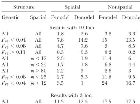
the literature; and (iii) as the model is specifically tai- Results on the whole set of simulations and on various

TABLE 1 Individual genotypes were obtained with the software

Easypop(Balloux2001) by simulating two populations

Average false classification rates (in percentage)

exchanging different numbers of migrants per

genera-for all simulated data sets and subsamples with

tion. In a first data set (referred to hereafter as set

various levels of genetic and spatial structure

A), the two populations are considerably differentiated

Structure Spatial Nonspatial (FST ⫽ 0.16), in a second set (B) the populations are

less differentiated (FST⫽0.06), and in a third data set

Genetic Spacial F-model D-model F-model D-model

(C), they are very weakly differentiated (FST⫽0.01). In

Results with 10 loci each set we haven⫽200 individuals (with 100

individu-All All 1.8 2.6 3.8 3.3 _{als per population) and L ⫽ 10 loci with Jl⫽1,...,L⫽ 10}

FST⬍0.04 All 7.8 14.2 15 13.5 _{alleles per locus. Individuals of each population were}

FST⬍0.06 All 4.7 7.6 9 8.5 _{randomly located on each part of an oscillating curve}

FST⬎0.11 All 0.3 0.3 0.2 0.2

on the unit square.

All m⬍12 2.3 1.9 11.4 6

The ability of the model to find the actual partition

All m⬍25 1.7 1.8 6.8 4.4

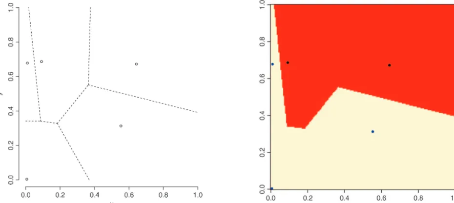
of space is illustrated in Figure 7, set A, which displays

All m⬎80 2.2 3 2.8 3

FST⬍0.06 m⬍25 2.7 5.3 11.8 9.5 the posterior probability␲(c(s)⫽k|t,z) for any pixel

FST⬍0.04 m⬍12 3.5 1 24 16.7 to belong to the two populations. We observe that the

true partition is very well detected. We obtained similar

Results with 3 loci

results on the two other data sets, although the

bound-All All 11.3 12.5 17.5 17.5

ary between the two domains was detected with less

The level of genetic and spatial structure increases withFST precision with data sets B and C (results not shown).

and decreases withm, respectively. Results are shown from _{We then quantitatively assessed how the level of} differen-1000 simulated data sets of 100 individuals in two populations,

tiation influences the precision in the estimation of the

withL⫽Jl⫽1,...,L⫽10 andL⫽3,Jl⫽1,...,L⫽10.

border. This can be viewed from the map of␦(s), where

␦(s) is any suitable measure of the dispersion of␲[c(s)|t,

z,K]. As␲[c(s)⫽j|t,z,K] is a probability measure on ture are given in Table 1. The quantiles at levels (0.1,

0.25, 0.75) of the empirical distributions of FSTand m {1, . . . , K} whose weights can be zero, the entropy is

not defined, and therefore we used instead were used to obtain subsets with various levels of genetic

differentiation and of spatial organization, respectively.

␦(s)⫽

兺

K

j⫽1

␲2_[c(s)⫽_{k|t,z,K] (8)}

The quantiles at probabilities (0.1, 0.25, 0.75) were

re-spectively (0.04, 0.06, 0.1) forFSTand (12, 25, 80) for

m. For instance, subsets for which the number of Voro- as an index of the dispersion of the distribution␲[c(s)⫽

k|t,z,K]. The right-hand side of Equation 8 is minimal

noi tilesmwere less than 12 correspond to highly

spa-tially structured populations, whereas those for which when all the colors have equal probability, which

corre-sponds to a flat posterior. Thus, the pointssfor which

m⬎80 correspond to loose spatial organization.

Exam-ples illustrating simulated data sets with various levels ␦(s) is high are those confidently classified, whereas

those where␦(s) is low correspond to poorly classified

of spatial organization are shown in Figure 6.

Results from the whole data set show that spatial meth- points that might correspond to transition regions or

to sparsely sampled regions. The maps of␦(s) given in

ods give lower FCR values than nonspatial methods and

that this trend is strengthened for a low number of loci Figure 8 for the three data sets show that the lower

values of ␦(s) are along the true line of discontinuity

(e.g., three loci). The improvement of spatial as

com-pared to nonspatial methods is the greatest when both (darker color), and that the accuracy in the estimation

increases with the level of differentiation between

popu-the level of spatial organization is large (m⬍12) and

the level of differentiation is weak (FST⬍ 0.04). lations.

Detection of migrants: Since populations exchange Hence, in addition to giving better results than the

spatial F-model for the estimation of the number of pop- migrants, it is sensible to assess whether the presence

of such migrants would affect the spatial detection of ulations, the spatial D-model compares favorably with

the spatial F-model for the assignment of individuals to genetic discontinuities and whether migrants could be

detected and spatially located by our method, for differ-their populations, even when the data depart from the

model assumed in the inference (c f. the data sets that ent levels of differentiation between populations.

To address these points, we mimicked the presence were simulated according to the spatial F-model).

There-fore in the following we focus on the spatial D-model of first-generation migrants in our previous data sets A,

B, and C by moving one individual from the upper only.

Mapping borders between populations:Mapping bor- population to the lower population and another one in the opposite direction. Figure 9 shows that the presence ders between populations represents one of the major

interests of our spatial model: it is presented through of these first-generation migrants did not affect the

Figure6.—Examples of simulated spatial organization of 100 individuals (black dots) into two populations (coded as two colors) with various levels of spatial dependence. This level is controlled by parameterm(number of Voronoi tiles). The nuclei of the tiles are not depicted for clarity.

to spatially locate the genetic discontinuity. The figure tion),L⫽Jl⫽1,...,L⫽ 10, and the level of differentiation

between populations was relatively low (FST⫽0.08). The

also shows that the two migrants are easily detected (i.e.,

visualized) for data sets A, B, and C. The population of true positions si were blurred by an additive noise εi

uniform on [⫺0.15, 0.15]2_{, so that the observed}

posi-origin of each migrant could be easily deduced from

its coloring pattern, including when more than two pop- tions were ti ⫽ si ⫹ εi. The model was first run

con-sidering that the given positions were true (ε⬅0) and

ulations shared the domain (results not shown).

Effect of errors on the locations of individuals: We in a second run the uncertainty was accounted for by

injecting the information that εi ⵑ Uniform[⫺0.15,

show here how errors on the locations of individuals may

lead to poor results and how accounting for errors in 0.15]2_{. We also considered the case where the true}

coor-dinates were used whereas wrong coorcoor-dinates were as-the positioning of individuals allows us to retrieve most

of the underlying signal. This question was addressed sumed, and finally we give the results for true

coordi-nates considered as true coordicoordi-nates. The results are through the analysis of a new set of simulations.

Three independent populations separated by straight summarized in Figure 10. It can be clearly observed

from the figure that accounting for uncertainty in the lines were positioned on the unit square. The number

pre-Figure7.—Maps of posterior probabilities, simulated data set A. The dashed green line depicts the true sine-shaped line of discontinuity.FST⫽0.16,L⫽Jl⫽1,...,L⫽10.

cision in the detection of the true borders when some includes 200,000 iterations and a short burn-in period.

The posterior distribution gave a mode atK⫽6, with

errors on the position of individuals exist (Figure 10,

line 1 vs. line 2). Moreover, adding position noise in a nonnegligible occurrence atK⫽5 (Figure 11). Then

the model was rerun along 50,000 iterations with a fixed the model does not alter the results for data sets without

position errors (Figure 10, line 3vs. line 4). value for K⫽ 6. Maps of the posterior probability for

any pixel of the domain to belong to each population could then be derived (Figure 12).

APPLICATION TO MONTANA WOLVERINES _{We also computed for each pixelsthe modal} popula-(GULO GULO)

tion, namely the populationkfor which␲(c(s)⫽ k|t,

z) is maximum (Figure 13). Two of the six inferred

We now analyze a previously published data set on

populations (i.e., Figure 12, populations 2 and 5) do wolverines (Gulo gulo), a medium-sized carnivore wildly

not appear to be the modal population for any pixel. distributed in North America. Wolverines are highly

mo-Moreover, these two populations have very low posterior bile, with the ability to disperse up to 300 km within a

probabilities and an analysis of a detailed map suggests year, but are also highly sensitive to habitat disturbance

that the areas of these populations are very similar. by humans. Eighty-nine individuals were sampled in

Although results from theNumber of populationssection

Montana and genotyped at 10 microsatellite loci

Cegel-suggest that one can be very confident in the spatial

skiet al. (2003). Samples are nearly evenly distributed

D-model to infer the right number of populations, we do over an area that corresponds to a landscape highly

not have straightforward interpretation of the “ghost” fragmented by human development and disturbance.

populations 2 and 5 (but seediscussionsection).

Using nonspatial Bayesian clustering procedures and

The spatial partition in four populations with high

assignment tests implemented in the programsStructure

posterior probabilities considerably (but not entirely) (Pritchardet al. 2000) andGeneclass(Cornuetet al.

decreased genetic structure within samples fromFIS ⫽

1999), Cegelskiet al. (2003) provided some evidence

0.180 to 0.088, with single-populationFISvalues ranging

for the existence of three populations of wolverines in

from 0.038 to 0.110. Hardy-Weinberg equilibrium could

Montana, withFSTvalues ranging from 0.08 to 0.10. The

not be rejected in two of the four inferred populations authors also provided some evidence for the

identifica-(Fisher’s exact test,P ⬎ 0.05;RaymondandRousset

tion of 11–22 migrants or offspring of migrants

(de-1995). Hence, our spatial method gives strong evidence pending on the method used for migrant detection).

for the presence of (at least) one more population than We reanalyzed the Wolverine data set (excluding one

previously detected using nonspatial statistical approaches sample whose spatial coordinates were missing) by

pro-(i.e., Figures 12 and 13, population 6). The three other cessing 10 independent MCMC runs of our spatial

populations occupy spatial domains rather similar to

D-model. We used priors onK- uniform between 1 and

Figure8.—Delineation of lines of discontinuities from the dispersion␦(s) of the posterior probability␲[c(s)|t,z].

The main added value of our spatial approach is thus map in Figure 2 ofCegelskiet al. (2003) shows that the

spatial domains of our populations 3 and 6 are separated the delineation of a fourth population located north

of population 3. Populations 3 and 6 were previously by a narrow extent of man-made habitats (i.e., grasslands

and grazing lands) that may have reduced wolverine

confounded using nonspatial methods. PairwiseFST

be-tween the four populations inferred by our method are movements.

Our spatial approach also allows detection of five indi-FST1–3⫽0.151,FST1–4⫽0.13,FST1–6⫽0.174,FST3–4⫽0.108,

FST3–6⫽0.079, andFST4–6⫽0.176. TheFST- value between viduals that genetically differ considerably from their

spatial neighbors (Figure 13). These individuals can be the previously confounded populations is thus the

low-est of all pairwiseFST. interpreted as first-generation migrants as suggested by

Figure9.—Maps of posterior probabilities␲(c(s)|t,z) in the presence of one migrant on both sides of the line of discontinuity. The migrants from the upper to lower popula-tion and from the lower to upper populapopula-tion are depicted by triangles and circles, respectively.

these putative individual migrants have been previously locus genotype data, without anya prioriknowledge on

detected byCegelskiet al. (2003). the populational units and limits. Once genetic

discon-tinuities have been detected and spatially located using the observed genetic data, accurate landscape

descrip-DISCUSSION _{tors implemented, for example, in a geographic}

infor-mation system (GIS) can be used to associate the inferred The two key steps of landscape genetics are the

detec-genetic discontinuities with landscape features and hence tion and location of genetic discontinuities and the

cor-generate hypotheses about the cause of genetic bound-relation of these discontinuities with landscape and

en-aries; seePiertneyet al.(1998) for an attempt in this

vironmental features. Efficient methods to achieve the

direction. first step have been lacking so far; our method provides

Our spatial method appears well suited for revealing the first efficient tool for locating genetic discontinuities

suit-Figure10.—Maps of the posterior probability␲[c(s)⫽k|t,z] when coordinatessiare blurred by a uniform noise. First row,

wrong coordinates, assumed true; second row, wrong coordinates, assumed wrong; third row, true coordinates, assumed wrong; fourth row, true coordinates, assumed true.FST⫽0.08,L⫽Jl⫽1,...,L⫽10. Dashed black lines are the true borders.

able approach for the detection of migrants (i.e., individ- individuals sampled in the northwestern United States

and genotyped at microsatellite markers (Cegelskiet al.

uals poorly genetically related to their spatial neighbors)

and their assignment to their population of origin. This 2003). In addition to the populations previously

identi-fied byCegelskiet al. (2003) using nonspatial methods,

rium with one another within populations (the effect of deviations from the second assumption is discussed further in this section). The accuracy of our method increases with the sampling effort (number of individu-als and loci) as well as the strength of the genetic discon-tinuity between populations. However, our analysis of both simulated and real data sets showed good perfor-mances of the method for data sets of standard size (e.g., 100 individuals genotyped at 10 loci with 10 alleles per locus), with mild to low levels of population

differen-tiation (e.g.,FST⬍0.1). Regarding individual sampling

strategy, efficient inference in landscape genetics im-plies random sampling across the entire study area and not just sampling some individuals in each of several

a priori defined populations (Manel et al. 2003). This

also holds for our spatial method. Because methods to treat spatially approximately evenly distributed individ-ual genetic data sets have not been available so far, such a sampling design has been rarely applied. We anticipate that our spatial method will stimulate population geneti-cists and ecologists interested in determining landscape and environmental factors influencing population

ge-Figure11.—Posterior distribution of the number of popula- _{netic structure to modify their sampling strategy. The} tions for the wolverine data. _{effect of a traditional sampling scheme (i.e., several}

groups of individuals collected on a limited area) on the performance of our method still needs to be assessed

our spatial approach allowed us to delineate a fourth _{using simulated data sets. However, preliminary tests}

population separated from others by a narrow extent _{suggest that this effect may be small if enough of such}

of human-made habitats. Our analysis hence strength- _{sampling groups have been collected.}

ens the conclusion that, even for a highly mobile species, _{An interesting feature of our method is its propensity}

habitat disturbance by humans may considerably limit _{to infer that several spatial domains that may be}

appar-movements and creates spatial genetic structure. Our _{ently unconnected within the sampling window can}

be-approach also allowed detection of migrants between _{long to the same population unit. This represents a}

populations that were not previously distinguished, us- _{significant advantage in comparison to previous}

meth-ing nonspatial approaches (e.g., Figure 13, two migrants _{ods that aimed to define population (or individual)}

originating from population 6). The overall larger num- _{groups and hence genetic discontinuities. Hence our}

ber of potential migrants detected by Cegelskiet al. _{method is capable of treating complex spatial situations.}

(2003) using assignment methods implemented in the _{In the meantime, we have demonstrated that our model}

package Geneclass (Cornuet et al. 1999) may be due _{does not artificially enforce a spatial substructure when}

to: (i) a lower power of our spatial method for detecting _{it does not exist (see especially caseK⫽1 in Figure 4).}

migrants and offspring of migrants, although this re- _{Another major advantage of our approach as a whole}

mains to be assessed; (ii) some Wahlund effect in at _{compared to earlier methods (Pritchard et al. 2000;}

least one population identified byCegelskiet al. (2003); _{Dupanloupet al. 2002; Falushet al. 2003) is that the}

and (iii) an excess of the first type of error (i.e., resident number of population units is treated here as an

un-individuals identified as migrants) produced by most known parameter. AlthoughCoranderet al. (2003) also

assignment methods, as previously shown from simu- did so, their method is not spatially explicit and aims

lated and empirical data sets (Berryet al. 2004;Paet- first at grouping populations rather than individuals.

kau et al. 2004). The exact behavior of our spatial Regarding inference of the number of population units,

method with respect to old migrants (e.g., F1, F2, and the spatial D-model was found to perform better than the

backcross migrants) still has to be assessed. Note that spatial F-model. The latter model tends to largely

over-these cases are explicitly treated in the admixture case estimate the number of population units, especially for

of theStructureapproach (Falushet al. 2003). low levels of population differentiation. To capture

sub-Although theoretically applicable to any type of quali- tle genetic structures, the F-model gives a rather loose

tative variable, our method was more specifically designed definition of what a population is. Embedding it in a

for genetic codominant markers (e.g., allozymes, micro- fully Bayesian model where the number of these loosely

satellites, single nucleotide polymorphisms). It assumes defined populations is itself unknown seems to place too

equilib-Figure12.—Maps of the posterior probability to belong to each population for the wolverine data. Unit of axis is kilometers.

agreement with those ofFalushet al. (2003), who found mated values, and graphical outputs about all

parame-ters involved can be derived from one single MCMC that, in a nonspatial context, the F-model was in general

more permissive than the D-model (additional popula- run. However, from a user point of view, it is more

con-venient to launch a first run processing all parameters tions being fitted to a data set), as it permits the

exis-tence of two or more populations with very similar allele in␪, from which onlyKˆ is derived, and then to launch

a second run withK⫽Kˆ, and from which all remaining

frequencies (particularly if the prior on the drift factor

is chosen to favor small values). parameters will be investigated. All computations

de-scribed in this article used the previous rule. It is worth We proposed a full Bayesian inference of the

parame-ters of our spatial model through MCMC simulations. mentioning that additional test computations performed

esti-Figure12.—Continued.

assumptions of our model were somewhat violated have in such situations, more could be gained from model

improvement than from inference algorithm improve-shown that results from one single run could be

mis-leading, as the Markov chain could get stuck to some ment.

Postprocessing issues were also encountered when local modes of the posterior. In this case we found,

in agreement withCorander et al. (2003, 2004), that computing modal populations on the wolverine data as

their number was smaller than the number of inferred processing several independent runs and ranking them

according to the posterior density could be an aid in populations. Such an issue has not been encountered

with simulated data. The reason why this has been ob-the interpretation of results. We believe, however, that

served in the wolverine data set has to be further as-sessed. However, we may speculate that, as often in the

MCMC algorithm for mixture models (Falushet al. 2003),

some rarely visited states lead to inferred populations that do not appear to be the modal population for any individuals. Such populations may be interpreted as spurious populations that have not been successfully removed by the MCMC algorithm (and, hence, as a con-vergence flaw of the algorithm) or as populations stand-ing for complex multimodality in the posterior. From a user point of view, these ghost populations have just to be ignored, and focus can be restricted to modal populations.

Some other forms of spatial dependence may occur in addition to that due to the presence of genetic discon-tinuities. These include isolation by distance between

individuals,i.e., a regular increase of differentiation

be-tween individuals with geographic distance due to

lim-ited dispersal (Rousset2000;Lebloiset al. 2003); kin

clustering,i.e., spatial clustering of highly related

indi-viduals at least before dispersal (e.g.,Kelly1994); and

a certain rate of selfing reproduction for some species

Figure13.—Map of the mode of the posterior probability

(WolfandTakebayashi2004). The problem of

isola-to belong isola-to each class for the wolverine data. Large character

tion by distance has been already mentioned by

Dupan-numbers indicate population labels. Arrows indicate putative

stepping-Geostatistics, edited byW. J. KleingeldandD. G. Krige. De Beers,

stone migration model, their method found significant

Cape Town.

clustering of populations in the absence of any genetic _{Balloux, F., 2001 EASYPOP (version 1.7), A computer program}

boundary. It is expected that isolation by distance, kin- for the simulation of population genetics. J. Heredi.92:301–302.

Berry, O., M. TocherandS. Sarre, 2004 Can assignment tests

clustering, or selfing decrease the performance of our

measure dispersal? Mol. Ecol.13:551–561.

spatial method since the latter assumes Hardy-Weinberg _{Besag, J., 1986 On the statistical analysis of dirty pictures. J. R. Stat.}

and linkage equilibrium among loci within populations Soc. Ser. B48(3): 259–302.

Blackwell, P., 2001 Bayesian inference for a random tesselation

separated by genetic discontinuities. In particular, it is

process. Biometrics57(2): 502–507.

expected that deviations from random assortment that _{Byers, S., andA. Raftery, 2002 Bayesian estimation and}

segmenta-are not caused by genetic discontinuity will tend to over- tion of spatial point processes using Voronoi tilings, pp. 109–121

inSpatial Cluster Modelling, edited by A. B.Lawsonand D. G. T.

estimate the number of population units (Pritchard

Denison. Chapman & Hall, London/New York.

et al. 2000;Falushet al. 2003). However, to which extent _{Cegelski, C., L. WaitsandJ. Anderson, 2003 Assessing population}

additional forms of spatial dependence would affect the structure and gene flow in Montana wolverines (Gulo, gulo) using

assignment-based approaches. Mol. Ecol.y12:2907–2918.

performance of our method to detect and locate genetic

Celeux, G., 1997 Discussion of the paper by Richardson and Green

discontinuities between populations still needs to be _{“On Bayesian analysis of mixtures with an unknown number of}

assessed, analyzing simulated data sets. Given the com- components.” J. R. Stat. Soc. Ser. B59(4): 775–776.

Celeux, G., M. HurnandC. Robert, 2000 Computational and

plexity of genetic data sets at highly variable markers,

inferential difficulties with mixture posterior distributions. J. Am.

our spatial model had to remain as simple as possible. _{Stat. Assoc.95(451): 957–970.}

A simple way to achieve spatial dependence was to as- Corander, J., P. WaldmannandM. Sillanpa¨a¨, 2003 Bayesian

anal-ysis of genetic differentiation between populations. Genetics163:

sume a dependence on the class variable and an

inde-367–374.

pendence of z(s) within populations. However, this _{Corander, J., P.Waldmann, P.Martinenand M.Sillanpa¨a¨, 2004}

basic model might be improved in several ways. For BAPS2: enhanced possibilities for the analysis of genetic

popula-tion structure. Bioinformatics20(15): 2363–2369.

instance,Allard andGuillot (2000) proposed in a

Cornuet, J., S. Piry, G. Luikart, A. EstoupandM. Solignac, 1999

different context a model where the population label _{New methods employing multilocus genotypes to select or exclude}

variable is not spatially dependent (unlike here where populations as origins of individuals. Genetics153:1989–2000.

Dawson, K., andK. Belkhir, 2001 A Bayesian approach to the

identi-the population variablecis spatially organized) and the

fication of panmictic populations and the assignment of

individu-datazare spatially dependent within populations. This _{als. Genet. Res.78:59–77.}

model tended to cluster samples in a way very different Dupanloup, I., S. SchneiderandL. Excoffier, 2002 A simulated

annealing approach to define genetic structure of populations.

from that of the current model. Although this model

Mol. Ecol.11:2571–2581.

is not straightforwardly transposable to genetic data, the _{Estoup, A., M. Beaumont, F. Sennedot, C.Moritzand J.Cornuet,}

introduction of within-population dependence while 2004 Genetic analysis of complex demographic scenarios:

spa-tially expanding populations of the cane toad, Bufo marinus.

keeping the spatial dependence of the class variable is

Evolution58:2021–2036.

certainly a promising way to improve spatial models for _{Falush, D., M. StephensandJ. Pritchard, 2003 Inference of}

popu-genetic data and, more specifically, to take into account lation structure using multilocus genotype data: linked loci and

correlated allele frequencies. Genetics164:1567–1587.

other forms of spatial dependence such as isolation by

Hurn, M., O. HusbyandH. Rue, 2003 A tutorial in image analysis,

distance, kin clustering, or selfing. _{pp. 86–141 inSpatial Statistics and Computational Methods(Lecture}

The whole computer code (including Fortran MCMC, Notes in Statistics). Springer, Berlin/Heidelberg, Germany/New

York.

postprocessing subroutines, and R data handling and

Ihaka, R., andR. Gentleman, 1996 R: a language for data analysis

graphical interfaces) used to carry out computations _{and graphics. J. Comput. Graph. Stat.5(3): 299–314.}

under our spatial model will be made available soon on Kelly, J., 1994 The effect of scale dependent processes on kin

selec-tion: mating and density regulation. Theor. Appl. Genet.46:32–57.

the web page of G. Guillot and Comprehensive R

Ar-Lantue´joul, C., 2002 Geostatistical Simulation. Springer,

Berlin/Hei-chive Network (IhakaandGentleman1996;R Devel- _{delberg, Germany/New York.}

opment Core Team2004) as an R package calledGene- Lawson, A., andD. Denison(Editors), 2002 Spatial Cluster Modelling. Chapman & Hall, London, New York.

land.

Leblois, R., A. EstoupandF. Rousset, 2003 Influence of muta-The wolverine data set was kindly provided by Chris Cegelski and _{tional and sampling factors on the estimation of demographic} Lisette Waits from the Department of Fish and Wildlife Resource, parameters in a ‘continuous’ population under isolation by

dis-tance. Mol. Biol. Evol.20:491–502. University of Idaho. We thank Stuart Baird for constructive comments

Manel, S., M. Schwartz, G. LuikartandP. Taberlet, 2003 Land-on the manuscript and Mark HewisLand-on for comments Land-on an earlier

scape genetics: combining landscape ecology and population ge-draft. G. Guillot thanks Joe¨l Chadœuf, Christian Robert, Eric Parent,

netics. Trends Ecol. Evol.18(4): 189–197. Olivier Franc¸ois, Jesper Møller, and Rasmus Waagepetersen for

stimu-Møller, J., and Ø.Skare, 2001 Coloured Voronoi tesselations for lating comments at various stages of this work. We also thank two

Bayesian image analysis and reservoir modelling. Stat. Mod.1:

reviewers and Laurent Excoffier as associate editor for constructive _231–252.

remarks. This work was partly supported by a grant to the authors _{Møller, J., andR. Waagepetersen, 1998 Markov connected} com-from Bureau des Ressources Ge´ne´tiques. ponent fields. Adv. Appl. Probab.30:1–35.

Nicholls, G., 1997 Coloured continuum triangulation models in the Bayesian analysis of two dimensional change point problems, pp. 143–150 inThe Art and Science of Bayesian Image Analysis: Leeds Annual Statistics Research Workshop, edited by K. V.Mardiaand LITERATURE CITED

R. G.Aykroyd. Leeds University Press, Leeds, UK.

Paetkau, D., R. Slade, M. BurdensandA. Estoup, 2004 Genetic

Allard, D., and G. Guillot, 2000 Clustering geostatistical data,

migra-tion rate: a simulamigra-tion-based exploramigra-tion of accuracy and power. Notes in Statistics), edited by Jesper Møller. Springer, Berlin/Hei-delberg, Germany/New York.

Mol. Ecol.15:55–65.

Rousset, F., 2000 Genetic differentiation between individuals. J. Evol.

Piertney, S., A. MacColl, P. Bacon andJ. Dallas, 1998 Local

Biol.13:58–62. genetic structure in red grouse (Lagopus lagopus scoticus): evidence

Stephens, M., 1997 Discussion of the paper by Richardson and from microsatellite DNA markers. Mol. Ecol.7(12): 1645–1654.

Green “On Bayesian analysis of mixtures with an unknown

num-Pritchard, J., M. StephensandP. Donnelly, 2000 Inference of

ber of components.” J. R. Stat. Soc. Ser. B59(4): 768–769. population structure using multilocus genotype data. Genetics

Stephens, M., 2000 Dealing with label-switching in mixture models.

155:945–959.

J. R. Stat. Soc. Ser. B62:795–809. RDevelopment Core Team, 2004 R: A Language and Environment

Tavare´, S., andO. Zeitouni, 2001 Proceedings of Saint Flour Summer for Statistical Computing. (http://www.R-project.org).

School in Probability and Statistics (Lecture Notes in Statistics).

Rannala, B., andJ. Moutain, 1997 Detecting immigration by using

Springer, Berlin/Heidelberg, Germany/New York. multilocus genotypes. Proc. Natl. Acad. Sci. USA94:9197–9201.

van Lieshout, M., 2000 Markov Point Processes and Their Applications.

Raymond, M., andF. Rousset, 1995 Genepop (version 1.2): a

popu-Imperial College Press, London. lation genetic software for exact test and ecumenicism. J. Hered.

Vounatsou, P., T. SmithandA. Gelfand, 2000 Spatial modelling

86:248–249.

of multinomial data with latent structure: an application to

geo-Richardson, S., and P.Green, 1997 On Bayesian analysis of

mix-graphical mapping of human gene and haplotype frequencies. tures with an unknown number of components. J. R. Stat. Soc. _{Biostatistics1(2): 177–189.}

Ser. B59(4): 731–792. _{Weir, B., andC. Cockerham, 1984 Estimating F-statistics for the}

Robert, C., and K. Mengersen, 1999 Reparameterisation issues _{analysis of population structure. Evolution38(6): 1358–1370.} in mixture modelling and their bearing on MCMC algorithms. _{Wolf, D., andN. Takebayashi, 2004 Pollen limitation and the} evo-Comput. Stat. Data Anal.29:325–343. _{lution of androdioecy from dioecy. Am. Nat.163:122–137.}

Roberts, G., andP. Dellaportas, 2003 Introduction to MCMC,

pp. 1–86 inSpatial Statistics and Computational Methods(Lecture Communicating editor: L.Excoffier

APPENDIX

Description of simulation study:The exact algorithm described inNumber of populationsis detailed in pseudo-code below:

doKin (1, 2, 5, 10)

do isim in 1:50

draw (m,u,c,d,f,fA,s) from ␲F_model(m,u,c,d,f,fA,s|K)

drawzfrom␲(z|␪)

simulate sample (␪)(Dt_model) from␲D_model(␪|z)

computeKˆD_model[isim]⫽posterior mode ofKin (␪)(

t)

D_model

simulate sample (␪)(Ft_model) from␲F_model(␪|z)

computeKˆF_model[isim]⫽posterior mode of Kin (␪)(

t)

F_model

enddo

plot histogram ofKˆ_D

plot histogram ofKˆ_F

enddo

In words, we simulated spatialized data sets with various sets of parameters and tried to retrieve these parameters, considered as unknown, via our algorithm with a special emphasis on the number of populations.

Details of MCMC computations: Six block updates (namely, those of u, c, p, f, fA, and s) do not change the

dimensionality of␪, and two updates (Kandm) are of jump type, increasing or decreasing the length of␪.

Update of drifts:This is done through Metropolis-Hastings updates, as described byFalushet al.(2003).

Update of frequencies in the ancestral population:This is done through Metropolis-Hastings updates, as described by

Falushet al. (2003).

Update of frequencies in the present-time population:This is done through Gibbs updates, as described byFalushet al.

(2003).

Update of the colors of tile:This is a Metropolis-Hastings update. We make componentwise updates ofc: sequentially

for each tile with colorcj, we propose a new valuec*j from the prior, namely␲(c*j ⫽l|K⫽k)⫽1/k.

This proposal is accepted according to the usual M-H acceptance probability

␣(␪,␪*)⫽1∧␲(t,z|K,m,u,c*,d,f,fA,s) ␲(t,z|K,m,u,c,d,f,fA,s)

, _(A1)