ABSTRACT
VARMA, SUYASH. On the Selection of Servers by Load Balancing of Network Traffic for Content-Streaming Data Centers. (Under the direction of Dr. Yannis Viniotis.)
Data-center networks are the buzzword nowadays in the field of enterprise networks, with technologies such as cloud computing offering indispensable services that are available anywhere and at any time. A data center network is the nexus through which such services flow. An increasingly popular such service over the past decade has been content delivery usually in the form of video streaming. Services such as Netflix and YouTube are prime examples. Moreover, the role of load-balancing of network traffic in a data-center network becomes even more essential when large chunks of video data need to be streamed out of a data-center network, from the servers to the gateways. It was interesting to discover that there are a lot of geographical load-balancing schemes but there is a conspicuous dearth of literature related to load-load-balancing of server to gateway traffic within a content-streaming data center.
In this dissertation, we propose a new approach to balancing“South-North” network traffic when streaming heavy content through a data-center network. Our approach assumes that, at the cost of redundancy, all the servers in the data center are capable of catering to any request for content and identifies all possible paths from servers through the switch fabric to the data center gateway. Once the paths are identified, our scheme takes measurements from the system and subjects these measurements to an algorithm that finds out the “load” on each path. The server corresponding to the path with the minimum load is then selected to cater to the incoming requests for content-streaming. To perform experiments to prove our hypothesis, we have written a discrete event simulator so that the usefulness of our scheme could be verified under different situations with arrival of requests, distribution of packets within the response, and duration of responses being a few of the variable parameters. Our algorithm has been compared with a Random Path Allocation scheme and this comparison highlights the necessity of a dynamic load balancing algorithm for selection of paths when catering to request for content.
© Copyright 2016 by Suyash Varma
On the Selection of Servers by Load Balancing of Network Traffic for Content-Streaming Data Centers
by Suyash Varma
A thesis submitted to the Graduate Faculty of North Carolina State University
in partial fulfillment of the requirements for the Degree of
Master of Science
Computer Networking
Raleigh, North Carolina
2016
APPROVED BY:
Dr. Harry Perros Dr. Mihail Sichitiu
DEDICATION
BIOGRAPHY
I have always believed that learning never stops. Every life experience teaches us a valuable lesson. It is our duty to inculcate these new lessons that we learn into our daily lifestyle and strive to be better tomorrow than what we are today.
ACKNOWLEDGEMENTS
This study has been the longest I have worked on a single project. It is also something I have given my utmost dedication and commitment to. There were phases in the course of this study when I was out of ideas or lacking in motivation, but I am very grateful to my advisor, Dr. Yannis Viniotis, who stood by my side when I needed guidance. He had a very calming effect on me every time I went to him with a problem I faced.
I am also grateful to my committee members, Dr. Harry Perros and Dr. Mihail Sichitiu for having agreed to guide me during the course of this study and for having tolerated the inconvenient deadline struggle that I faced.
TABLE OF CONTENTS
LIST OF FIGURES . . . vi
Chapter 1 Introduction . . . 1
1.1 Data Centers . . . 2
1.1.1 Data Centers - What are they and What Kinds are there? . . . 2
1.1.2 Data Center Topologies . . . 4
1.1.3 Data Center Network Traffic . . . 6
1.1.4 Content-Streaming Data Centers . . . 7
1.2 Load Balancing . . . 8
1.2.1 Meaning of Load Balancing . . . 8
1.2.2 Common Approaches to Load Balancing . . . 8
1.2.3 Load Balancing for Content-Streaming Data Centers . . . 10
1.3 The Bigger Picture . . . 11
Chapter 2 The South-North Load Balancing Problem. . . 12
2.1 Problem Statement . . . 12
2.1.1 Concise Problem Statement and Detailed Description . . . 12
2.2 Why is the Problem Important? . . . 13
2.2.1 Growing Popularity of Video Internet traffic . . . 13
2.2.2 Dearth of Load Balancing Schemes for Data Centers in South-North Di-rection . . . 14
2.2.3 What if There is No Load Balancing? . . . 14
2.3 Related Work . . . 15
Chapter 3 The Path-Based Load Balancing by Server Selection Algorithm . . 19
3.1 Network topology . . . 19
3.1.1 Topology Description . . . 19
3.1.2 Topology Justification . . . 20
3.2 Algorithm Description . . . 21
3.2.1 Assumptions and Supporting Facts . . . 21
3.2.2 Algorithm Details . . . 22
3.2.3 Mapping of Load Balancing Algorithm to Feedback Loop . . . 25
3.3 Experimental Setup and Evaluation . . . 26
3.3.1 Simulation Setup . . . 26
3.3.2 System Stability . . . 26
3.3.3 Experiments, Justifications and Results . . . 27
3.3.4 Limitations of the Algorithm/Experimental Setup . . . 41
Chapter 4 Conclusion and Future Work . . . 42
4.1 A Summary of Findings . . . 42
4.2 Future Work . . . 43
LIST OF FIGURES
Figure 1.1 Fat Tree Topology . . . 4
Figure 1.2 Clos Topology . . . 5
Figure 1.3 Modular Topology . . . 6
Figure 1.4 Dynamic Load Balancing Approaches . . . 10
Figure 2.1 South-North Traffic . . . 13
Figure 3.1 Datacenter Network Topology . . . 20
Figure 3.2 The Feedback Loop . . . 25
Figure 3.3 Cumulative Throughput . . . 33
Figure 3.4 Per Path Load . . . 34
Figure 3.5 Per Path Load-Random . . . 36
Figure 3.6 Access Layer Queues-100% Utilization . . . 36
Figure 3.7 Distribution Layer Queues-100% Utilization . . . 37
Figure 3.8 Access Layer Queues-90% Utilization . . . 38
Figure 3.9 Distribution Layer Queues-90% Utilization . . . 38
Figure 3.10 Access Layer Queues-80% Utilization . . . 39
Figure 3.11 Distribution Layer Queues-80% Utilization . . . 39
Figure 3.12 Access Layer Queues vs System Utilization . . . 40
Chapter 1
Introduction
It is sometimes hard to realize that something as simple as watching a movie on Netflix or playing your favorite song on YouTube actually has a fairly complicated process to it. Which is why it is a popular saying that the Internet has made life easy. Well, most lives. Throughout the course of this write-up, the reader will see just how much emphasis is laid on the fact that there is a huge quantity of data being sent across the Internet between geographically different locations. It is also easy to observe that Content Delivery is a large chunk of this data. Today’s tech savvy population that uses the Internet is familiar with facts such as video files are sig-nificantly larger than text files. And if we talk about well-established Content providers with millions of subscribers, such as YouTube, Netflix, Amazon Video, Hulu, Dailymotion, Vimeo and many more, there is no question to the fact that there indeed is a massive quantity of video data being served over the Internet. If we add to that music streaming services such as Spotify, iTunes and Saavn, we are talking about unimaginable number of bits being transmitted over the Internet every second. Moreover, the end-users having paid for these services, expect seamless streaming all the time every day of the year.
able to serve the customer base satisfactorily. Every such service provider employs thousands of network administrators who work towards making all this possible. To ease out the lives of such service providers and their network administrators, this thesis presents a small stepping stone in the direction of Load Balancing of Network traffic within a Content-Streaming Data Center. The following sections and subsequent chapters will explain how.
1.1
Data Centers
1.1.1 Data Centers - What are they and What Kinds are there?
Before we head into adding optimizations to how a data center should work, it is important to get the gist of what a data center is. As defined by [1], “Data centers are the home to criti-cal computing resources in controlled environments and under centralized management, which enable enterprises to operate around the clock or according to their business needs.” The com-puting resources this definitions talks about are essentially servers running operating systems that are a home to applications hosted by the data center, the data center network infrastruc-ture enabling communication between these servers, storage infrastrucinfrastruc-ture that actually hosts all the data present in the data center and a storage area network. All these resources work towards running applications which provide services the data center has advertised.
Another common and simple definition to data centers from [2] states that “a Data Center refers to any large, dedicated cluster of computers that is owned and operated by a single or-ganization.” These definitions do a pretty good job of defining a data center and the resources it needs for its operation. One of the most important resources is the data center network itself which links the servers to each other and to the outside world. Although, the network is nothing but a group of network devices such as switches and routers connected in a certain method, meant for forwarding network traffic, its deployment at a scale as large as a data center with thousands of servers makes it a very complicated network. Efforts to simplify this network resulted in certain popular data center network topologies such as Fat-tree topology, Clos topology and so on. These have been described in detail in Section 1.3.
Although data centers can be customized specifically to the requirements of the organization that owns them, there are still certain popular use cases of data centers which are usually the following.
1. University Campus Data Centers
departments, academic resources such as online libraries and lectures and so on. These data centers also run basic applications such as Hadoop/Map Reduce chiefly for the purpose of academic research.
2. Private Enterprise Data Centers
Private Enterprise Data Centers are owned and operated by enterprises and the services offered by such data centers are accessible only within the organization. To an extent their purpose is similar to a University Campus data center and resources unique to the organization and hosted in these data centers, varying from employee directories to intellectual property and financial resources.
3. Cloud Data Centers
This kind of data centers is the one with all the industrial focus since the past decade or so. These data centers are deployed at very large scales and boast of services such as “Software as a Service”, “Platform as a Service” and “Infrastructure as a Service”. The term “Cloud” indicates that these data centers have applications running or content stored, which is accessible directly over the Internet and the subscribers to these services are customers of the organization that owns the data center. A few examples of services offered by them are Amazon EC2, Microsoft Azure, VMWare ESX hypervisor and so on. They can be further divided into two broad categories.
Customer-facing applications
This category of Cloud data centers hosts applications which provide services that end-users subscribe to and pay for. The characteristic of such data centers is that they are directly accessible to the customer base over the Internet. Good examples are Netflix, Spotify, YouTube apart from the ones mentioned before.
Large scale data-intensive tasks
This category of data centers is meant for processing massive amounts of data by distributing it between servers. Typical examples are indexing web pages and data compression, which use MapReduce style applications to meet the requirements.
1.1.2 Data Center Topologies
Data centers can be customized as per the requirements of the organization, and this heuristic applies to their topology too. However, modern-day large scale data centers are based on one of the following three topologies depending on the scale and needs of the data center.
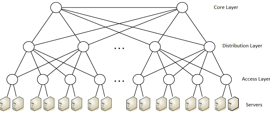
1. Fat-tree topology
Figure 1.1 demonstrates a full-fledged Fat-tree data center topology with three layers
Figure 1.1: Fat Tree Topology(Image Courtesy: doi.ieeecomputersociety.org)
could not forward traffic up to the Distribution layer using “fatter” links. However, as the amount of network traffic increased further, the traffic being forwarded via the Dis-tribution layer needed to be further aggregated using even fatter links (around 40 Gbps), giving rise to the Core Layer. As of today, these high link capacity switches are par for the course.
However, it can be observed from Figure 1.1 that such a data center topology is vulner-able to loops. To solve this problem, usually network administrators either activate the Spanning Tree Protocol, which in turn cuts down the possible uplinks/downlinks for a switch, or aggregate links together to increase link capacity as well as prevent loops, or design the data center network as a layer 3 routed network.
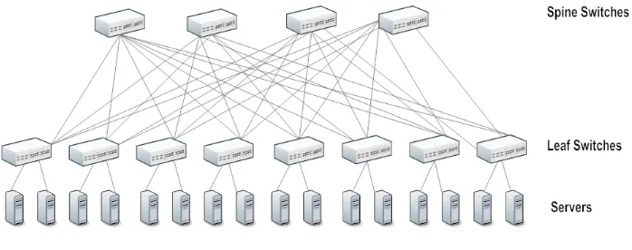
2. Clos topology
Figure 1.2 demonstrates a standard Clos topology for data centers. Each server is
con-Figure 1.2: Clos Topology
nected to a Leaf switch, which are in turn connected to all the Spine switches in the topology forming a full mesh. The Leaf switches are only connected to the Spine switches and not to each other. The Spine switches enable communication between servers and communication to an upstream gateway. The total number of links between the Leaf switches and the Spine switches is the product of the number of Leaf switches and the number of Spine switches. The advantage of a Clos topology is that a larger number of very similar switches can be used to completely construct a tree-like network, which would otherwise require more expensive higher capacity network switches.
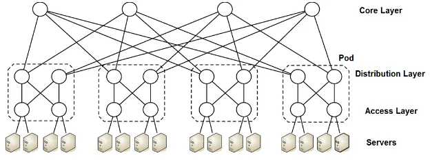
An important variant of the Fat-tree topology is the Modular topology in which Access
Figure 1.3: Modular Topology
layer and Core layer switches are arranged in pods usually consisting of two Access layer switches and two Distribution layer switches, as demonstrated in Figure 1.3. The dif-ference between this and the conventional three-layered topology is just that it has the same number of Distribution switches as the Access switches in a pod, which makes the network redundant and comes in handy in case of a link down or a switch failure. Apart from that, the Modular topology does not impose any regulations on the link speeds at every layer.
1.1.3 Data Center Network Traffic
East-West traffic refers to any network traffic between servers within a data center. We know that servers in data centers sometimes work together in a distributed way to be able to provide a service. For example, when a form filled by an end-user (a client) on a webpage needs to be validated, the information filled in by the user travels over the Internet to a data center which has stored information and credentials corresponding to this user. However, his name might be stored at a location accessible to one server whereas his age might be stored at another location accessible to another server. In such a case, the servers obviously need to talk to each other before they are able to validate the user information and send out an appropriate response back to the user. In order to be able to do that in a coordinated and effective manner, these servers generate network traffic addressed to each other. Network traffic of this kind within a data center is what is usually referred to as East-West traffic. It is also known as Server-Server traffic.
On the other hand, when the servers are done talking to each other and have prepared an appropriate response for the client who had requested the server for a service, this response needs to be sent out through the data center network followed by a Wide Area Network and ultimately to the client. This category of network traffic which essentially carries requests to the servers and responses from the servers is referred to as South-North Traffic or Server-Client traffic. It is important to observe here that when we talk about content streaming data centers, there is an enormous amount of South-North network traffic simply because of the fact that large content files such as songs or videos are being streamed out from the servers towards the network gateway.
1.1.4 Content-Streaming Data Centers
Now that we have understood what a data center is, what its architecture is like, how it oper-ates and what are its network traffic characteristics, the next question that arises is what is so different about Content-Streaming Data Centers. This section addresses this specific question.
the content corresponding to the request from the storage infrastructure and generates a flow of packets which contain the content requested. This flow then constitutes one of the thousands of similar flows that move in the South-North direction from the Servers to the Core switches to the gateway and ultimately to the users who clicked on video links on YouTube [4].
Content-streaming data centers usually also have redundant storage infrastructure to make sure the data center operates in a fail-safe manner and also so that all servers have access to all content that can be requested.
1.2
Load Balancing
1.2.1 Meaning of Load Balancing
Load Balancing refers to the act of distributing a task equally between a given number of resources that are capable of doing the task, so that each resource does about the same amount of work as the other resources. Having said that, “Load” can have multiple definitions by itself and so can “Balancing.” For someone “Load” can refer to bits, whereas for someone else, “Load” can refer to bits per second and for someone else “Load” can refer to the number of people standing at each checkout counter in a grocery store. Similarly, “Balancing” can also have multiple definitions. While the essence of “balancing” is in equally dividing the total load between the resources available, there might be situations when resources doing similar amount of work but not exactly the same amount of work might still be considered balanced in load.
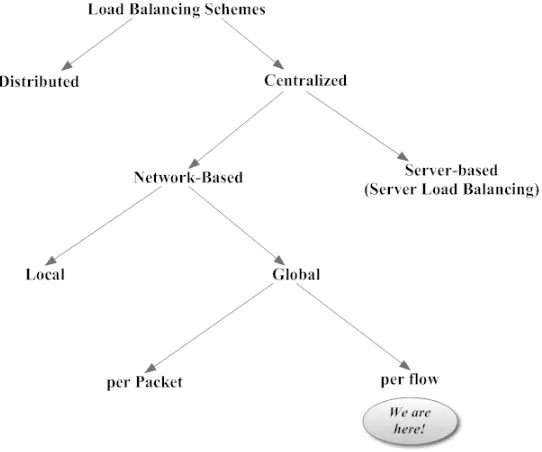
1.2.2 Common Approaches to Load Balancing Load Balancing schemes can be broadly classified into two
kinds-1. Non-dynamic Load Balancing Schemes
ECMP (Equal Cost Multipath). Under this scheme, flows are balanced between paths by hashing flow-related data, such as Source IP address or Destination L2 address, from packet headers. Thus, each flow gets assigned a particular path. However, ECMP is also prone to situations when a large flow sometimes called an Elephant flow [5] gets allocated a particular path. This flow would hog the bandwidth on its path and result in an imbalance between all the available paths as far as average load on each path is concerned. Given these potential issues with non-dynamic schemes, a need was felt for having dynamic schemes that actually take measurements from the System and make an intelligent scheduling decision in order to balance load.
2. Dynamic Load Balancing Schemes
Dynamic schemes provide what non-dynamic schemes had missing. Dynamic schemes ac-tually have an algorithm running behind the scenes which decides on metrics to monitor and then periodically takes measurements of these metrics from the System. Based on these readings, they make an informed decision about which resource needs to handle the next task at hand. Such dynamic schemes can be classified into multiple categories as demonstrated by Figure 1.4.
Figure 1.4: Common Approaches to Dynamic Load Balancing
1.2.3 Load Balancing for Content-Streaming Data Centers
1.3
The Bigger Picture
During the initial phase of research on this topic, a lot of time was spent on looking for previous research work that addresses Load Balancing in a Data Center Network in the South-North direction. As stated before, we found a few schemes that looked to address Load Balancing for Content Streaming Data Centers by balancing the load between multiple data centers, based on different parameters. For example, Torres et al in [4] present intelligent and plausible con-jectures about how Google balances the more than two billion requests for YouTube videos between data centers located all over the world. They study metrics such as user proximity, popularity of video content in a certain geographical area and so on. Similarly, Zhang et al in [9] do an extensive study on YouTube and how YouTube data centers balance load between its themselves. They come up with interesting findings that indicate that YouTube employs a location-agnostic proportional load balancing strategy between its data centers to service user requests from all over the world. However, none of these studies talked about a dynamic load balancing scheme that operated within a content streaming data center. It is possible and also very likely that tech giants such as Google (YouTube) and Netflix already have proprietary algorithms running in their data centers that take care of load balancing. However, these algo-rithms have not been made public.
Chapter 2
The South-North Load Balancing
Problem
In this chapter we address the specific problem of Load Balancing in South-North direction in a Content Streaming Data Center Environment. This chapter gives the readers a detailed description of the problem statement, the importance and necessity of addressing this problem and finally some exceptional research work done in the field of Load Balancing in Data Centers, which helped us find a direction as to how to come up with a Load Balancing scheme of our own.
2.1
Problem Statement
2.1.1 Concise Problem Statement and Detailed Description
The Problem Statement To devise a Path-based Load Balancing Scheme that performs Server selection for new requests for Content by balancing South-North traffic in a Content-streaming data center environment
South-North traffic, the problem statement makes it an objective to balance the load carried by each of these paths.
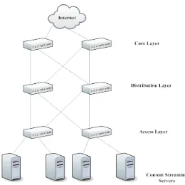
Figure 2.1: South-North Traffic in a Datacenter
Hence, whenever a new request for content arrives, an algorithm needs to take a few mea-surements from the System and allocate a path to the network traffic generated for the new request. Moreover, as described later in Chapter 3, since each path emanates at a Content-streaming Server, selecting a path for the new request effectively implies selecting a physical server for the new request.
2.2
Why is the Problem Important?
2.2.1 Growing Popularity of Video Internet traffic
Internet traffic as of 2014 and is predicted to constitute 80 per cent of all consumer Internet traffic by 2019. Every second, nearly a million minutes of video content will cross the Internet by 2019. Also, by 2019, as much as 72 per cent of all Internet video traffic will cross Content Delivery Networks, up from 57 per cent in 2014. These figures demonstrate beyond question the growing popularity of Video Internet Traffic and also demonstrate the need for high efficiency when streaming out content from data centers.
2.2.2 Dearth of Load Balancing Schemes for Data Centers in South-North Direction
Load Balancing has traditionally been a very popular research field in every domain that has a task that needs to be completed and multiple resources available to do this task. The same is true with Data Center networks simply because of the fact that there is a lot of network traffic and there are multiple paths that this traffic can take. With content-streaming data centers, the act of Load Balancing can and actually is done at two different levels. Since users requesting content such as videos over the Internet expect a fast response, the majority of load balancing research for Content Streaming data centers has been done on geographical load balancing as described in Section 1.3. There is not much literature to be found as far as Load Balancing of content-carrying network traffic within a Content Streaming data center is concerned. This fact highlights the importance of the problem we are going to address in the coming sections.
2.2.3 What if There is No Load Balancing?
2.3
Related Work
The following section describes some of the very recent and very clinical research work done on Load Balancing in Data Center networks. Although these works are individually not specific to Content Streaming, they give a lot of useful insight about the intricacies of balancing network traffic load, things that need to be taken care of and possible scenarios where compromises are needed. They have been described in some detail here.
Dynamic Load Balancing Without Packet Reordering - FLARE
This paper [12] introduces a dynamic but local load balancing scheme for ISP networks that uses a traffic splitting algorithm that operates on bursts of packets chosen carefully in order to avoid packet reordering. Their scheme, better known as FLARE (Flowlet Aware Routing Engine), introduced to us the concept of flowlets.
Since flows can have a variety of sizes and may not provide a very high granularity while load balancing, the objects of load balancing in this scheme are flowlets instead of flows. Flowlets are defined by bursts of traffic that are spaced by a minimum time interval chosen to be larger than the maximum delay difference between the possible parallel paths to the destination. This in essence is a definition designed for the purpose of avoiding packet reordering in the process of load balancing.
This paper highlights the need for dynamic load balancing in an ISP network. This need arises when there is a sudden burst of traffic, or when there is a link failure. The FLARE algorithm is deployed in a distributed fashion, at all routers in the ISP network.
The algorithm takes as input a split vector that can change over time. The split vector de-fines the individual weights to be assigned to each of the possible links to send out the packet. Ideally, the long-time average utilization of the links should be distributed as directed by these weights once the load balancing algorithm has been deployed. FLARE uses periodic pings to estimate the delay difference between the possible parallel paths and normalizes this estimate using exponential moving average.
traces to show that flowlets also exist in non-TCP traffic.
The authors have produced experimental results to show that FLARE has a very minimal impact on TCP timers and congestion control. However, since there is scope for packet reorder-ing in this scheme, TCP congestion control is triggered if at all packets happen to get reordered due to factors such as queuing delay at the network devices in the path, making this scheme vulnerable to false TCP congestion control alarms.
CONGA: Distributed Congestion-Aware Load Balancing for Datacenters
This very recent research paper [7] introduces to us a network-based distributed congestion-aware load balancing mechanism for data centers. The objective is to balance network traffic between paths between a pair of leaf switches in a leaf-spine topology. The scheme makes use of the concept of flowlets by splitting TCP flows into flowlets. This gives higher granularity and resilience against the size of each flow. Effectively, the network traffic entity that becomes the object of their load-balancing algorithm is these flowlets, each of which is allocated a particular uplink at the source leaf switch. The scheme relies on feedback from remote leaf switches in order to decide which uplink to send out a particular flowlet from. For further understanding, it is necessary to understand how the authors have defined flowlets.
Flowlets are bursts of packets from a flow that are separated by a large enough gap, say G. If the idle time between two consecutive bursts is greater than the maximum difference in latency among all possible paths to the concerned destination leaf switch, then the second burst can be referred to as a separate flowlet and can be sent using a different path from the first flowlet without causing any packet reordering. This results in higher granularity, resulting in more precise load balancing without causing packet reordering. Packet reordering is something that we do not want because it jolts TCP connections, which in turn, sets off a false alarm for TCP congestion control to begin, thereby decreasing effective throughput of the network. The idle time period (G) required between two bursts to classify them as separate flowlets has been set experimentally.
The source leaf switch (and any leaf switch can be a source) knows the ultimate destination leaf for each packet it sends out. How this mapping between end-point identifiers and their location (the leaf switch where the end-point rests) has not been described in the paper.
A “Congestion-to-leaf” table present at every leaf switch has entries for each possible uplink out of the source switch for each destination leaf switch. These entries are a measure of the maximum congestion along the entire path. If more than one path is possible originating at the same uplink from the source switch, then the spine switches pick any one of the possible next hops using standard ECMP hashing (and update another field in charge of indicating the path congestion metric, called CE field in the VXLAN header if the selected link’s congestion metric is higher than the field’s current value). The uplink is chosen by minimizing the maximum of remote congestion metric AND local congestion metric for each uplink. The mechanism to inform a source leaf switch about congestion on the possible uplinks is using a feedback loop from the destination leaf switch.
CONGA’s approach violates the packet reordering principle by leaving a scope for packet reordering. Even if two consecutive bursts are identified as flowlets based on the idle period between them, it is theoretically still possible that the second flowlet reaches the destination leaf switch before the first flowlet because of reasons such as queuing delay in any of the network devices present in the chosen path, thus resulting in packet reordering. Thus, from the research work described in this paper, we were able to realize that flowlets are something we will not be able to implement in our load balancing solution chiefly because there is a potential risk of packet reordering and also because the granularity of measurements required is something that might not be possible in software.
Hedera: Dynamic Flow Scheduling for Data Center Networks
flow on the best possible ECMP path.
Chapter 3
The Path-Based Load Balancing by
Server Selection Algorithm
This chapter forms the core of the thesis and describes the details of the assumptions made, the implementation done, the choices made and the reasons behind these choices. It begins with description of the network topology used, moves on to details of the algorithm developed and finally describes the experiments and results done to validate the effectiveness and the necessity of the algorithm.
3.1
Network topology
3.1.1 Topology Description
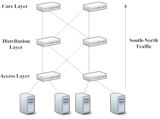
For the experiments, a modular three-layered network topology has been used. As can be ob-served in Figure 3.1, the topology includes four Servers for the purpose of Content Streaming and a switching fabric with two Access Layer switches, two Distribution Layer switches and two Core Layer switches. Each of the two switches at the Access Layer communicates with two servers.
Figure 3.1: Datacenter Network Topology Deployed for Experimentation
3.1.2 Topology Justification
Three-layered topologies are what data centers have been built upon traditionally due to the fact that there are just so many servers generating traffic that its aggregation needs to be done over three layers. Although with increasing link speeds that modern day switches now support, the traditional three layer topology has begun to collapse back into two layers (Clos Topologies) as described in Section 1.1.2, it is still more logical to devise a content streaming load-balancing scheme for the traditional three-layered topology which could eventually be extended to Clos topologies.
3.2
Algorithm Description
3.2.1 Assumptions and Supporting Facts
Listed here are the basic assumptions that have been made by the algorithm and supporting facts for the experimental setup.
1. There is a one to one correspondence between the terms “request” and “flow”. In other words, a “request” for content from an end-user generates a single “flow” of network traffic carrying the requested content and some metadata. A good example can be when an end-user clicks on a YouTube video that he wants to watch, it generates a “request” which eventually results in a “flow”.
2. Each request is first received by a central controller which runs the load-balancing al-gorithm upon arrival of the request, allocates a path for the flow corresponding to this request and then forwards the request to the corresponding content-streaming server, which in turn generates a flow to cater to the request. A management network allowing transportation of measurements from the switches and servers to this central controller has also been assumed.
3. All the four content-streaming servers are linked to a common storage infrastructure that stores all the content advertised by the datacenter. This makes them capable of catering to all possible requests for content that can be asked of the data center.
4. A content-streaming server can cater to more than one request simultaneously. Be-sides this, multiple request for the same content are possible and can be served by the same/different servers.
5. Once packets belonging to a flow reach the Core layer switches in the topology, they are assumed to be routed to a gateway router and eventually to the end user through a network such as the Internet.
6. The flows generated by the servers have a field as part of their metadata which can be used to identify what path they belong to. This field is used by the switch fabric to route packets of a flow to the intended queue.
8. The algorithm is a flow-based algorithm. In other words, the algorithm can only be run when a new request arrives and a corresponding flow needs to be generated. The algorithm has not been designed to be more granular than this.
3.2.2 Algorithm Details
As described in Section 2.1, the algorithm needed to be one that would balance load between all possible paths from the content-streaming servers to the Core Layer of the switch fabric. Having said that, it is important to have exact definitions for terms such as “Path” and “Load” before the description of the algorithm.
What is a Path? Any combination of three links that leads from a Content-streaming Server to any of the Core layer switches. Refer to Figure 3.1.
What is Load? The time-averaged cumulative number of bits recorded for each path. At any time instanttn, the time-averaged Cumulative Bits (Li) on a pathiis given by:
Li(tn) =
Bi(tn)−Bi(t0)
tn−t0
(3.1)
whereBi(tn) is the cumulative number of bits that have been allocated to Pathiby time instant
tn and t0 is the time instant when the first packet was received at any of the Servers for Path
iduring the course of the simulation.
When is the Load “Balanced”? It is also important to address when the load-balancing algorithm can be declared to have achieved success. The algorithm takes some time before it starts effectively balancing load between all the paths. The reason for this has been explained in Section 3.2.2. However, having said that, apart from this initial time window, the algorithm can be evaluated for load-balancing at pretty much all the time instances during the simulation as long as new flows are coming in. The definition of the load being “balanced” is something which is so open to different interpretations that it is tough to define it in numbers. However, the experimental results that follow in Section 3.3.2 provide guarantees of per path load with a certain confidence.
The Role of Cumulative Number of BitsFor each path, keeping a track of the cumulative number of bits that have been through it at any time instant since the beginning of the time window is essential simply because of the fact that the load-balancing algorithm defines load as the time-averaged cumulative number of bits per path and in order to be able to balance this definition of load, one needs to measure this particular statistic. The algorithm does that at the Servers by recording the number of bits previously allocated to each path. The algorithm then uses this parameter to allocate one of the sixteen possible paths to a new flow.
The Role of Queue Lengths While load balancing of network traffic in the data center is something the algorithm looks to achieve, a significant purpose behind load-balancing is to be able to observe shorter queue lengths at links of switches at all layers. This in turn leaves more buffer memory in the switches for other applications to use. So, it is logical to weigh in the current status of queues in terms of their length and make this a deciding factor too when allocating a path to a new flow, especially because of the fact that a cumulative measure of a parameter is not necessarily an accurate indication of the current state of the system. This is why the algorithm explicitly measures the current queue lengths of all the queues present in the topology and decides the candidacy of a path to be able to serve a new flow by looking at the queue lengths at each of the three links in the path, besides the load on the path.
The algorithm weighs in the contribution of both the above factors by allocating a weight factor of α to the Cumulative number of bits seen at a given path and (1−α) to the Queue Lengths on this path. The following set of equations better demonstrates the crux of the algorithm. The Load on a Path iat any time instantt is given by Xi(t):
Xi(t) =α∗[
Bi(t) n P
i=1
Bi(t)
] + (1−α)∗[ nQi(t)
P
i=1
Qi(t)
] (3.2)
where,
Bi(t) = t X
t0=0
bi(t0) (3.3)
and
Qi(t) =
3
X
k=1
qk(t) (3.4)
wherebi(t0) is the number of bits allocated at the Servers at time instantt0 for the pathi and
qi(t) is the queue length of the queue corresponding to path i at layer k. For the purpose of
simplicity, the layers of topology with queues relevant to our discussion, that is the Servers, the Access Layer and the Distribution Layer have been represented by k.
Also, the value of α has been empirically fixed at 0.9 because the focus of the algorithm is to balance the load as defined by Equation 3.1 between all the possible paths while taking care of the off-chance that a path with the least load happens to have an exceptionally large queue length. This is why the role of the queue lengths along a path, while important, is minimal. Algorithm 1 describes the pseudo code of the Load Balancing algorithm.
Algorithm 1 The Load Balancing Algorithm 1: procedure LoadBalancer
2: pathN o←1
3: totalQueueLength←0
4: while pathN o≤totalP athsdo 5: layer← 1
6: totalLayers←3 7: pathQueueLength← 0
8: whilelayer ≤totalLayers do
9: pathQueueLength←pathQueueLength+f indQueueLength(path, layer) 10: layer ←layer+ 1
11: end while
12: totalQueueLength←totalQueueLength+pathQueueLength
13: pathN o←pathN o+ 1 14: end while
15: pathN o←1
16: while pathN o≤totalP athsdo
17: if totalCumulativeBits6= 0 AND totalQueueLength6= 0 then
18: Load ← α ∗ (pathCumulativeBits/totalCumulativeBits) + (1 − α) ∗ (pathQueueLength/totalQueueLength)
19: else
20: if totalCumulativeBits6= 0 ANDtotalQueueLength= 0then 21: Load←α∗(pathCumulativeBits/totalCumulativeBits) 22: else
23: Load←(1−α)∗(pathQueueLength/totalQueueLength) 24: end if
25: end if
28: pathN o←1
29: while pathN o≤totalP athsdo 30: minLoad←Load[P ath1] 31: if Load < minLoad then 32: minLoad←Load 33: end if
34: pathN o←pathN o+ 1 35: end while
36: Return path with minimum Load 37: end procedure
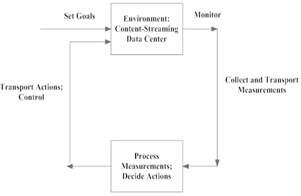
3.2.3 Mapping of Load Balancing Algorithm to Feedback Loop
Figure 3.2: The Feedback Loop
of a management network, we must have an algorithm which processes these measurements, which in our case is the Load Balancing algorithm described in Section 3.2.2, and finally we must have identified the actions we need to take based on the algorithm, which in our case is the allocation of flows to the best path decided by the Load Balancing algorithm.
3.3
Experimental Setup and Evaluation
3.3.1 Simulation Setup
To test the algorithm and gather results, a Discrete Event Simulator has been written that emulates a data center environment. The simulator has been written in C and operates on an event list which is a linked list that lists all the events that are going to happen in the simulation chronologically[18]. As the simulation moves ahead in time, events that occur also trigger the scheduling of more events at some point in time in the future. Apart from this event list, the simulator includes implementation of multiple queues that represent each uplink of switches at each layer of the topology. Based on the principles of discrete event simulations, events such as insertion of a packet into a queue, deletion of a packet from the previous queue and so on were defined and logic was written that took care of such sequences.
Each run of the simulator includes one instance of traffic generation and its flow through the datacenter topology with path selection for each flow dependent on the Load Balancing algorithm and one instance of traffic generation and its flow through the datacenter topology with random path selection. Each run of the simulation generates a number of output files which are read and comprehended by bash shell scripts that gather results from these files. These results are then represented graphically.
3.3.2 System Stability
In any queuing system, it is essential to ensure System Stability in order to avoid queues that keep increasing in size gradually, leading to a very undesirable state. The way to ensure System Stability is by having an average Arrival rate (λ) less than or equal to the Service Rate (µ). This ensures that packets are served at an equal or higher rate than at which they arrive on an average, thus ensuring finite queues that do not constantly keep increasing in size. So, the condition for stability is:
In our System, it is easy to observe that the Arrival rate (λ) can be defined in terms of the rate at which the Flows are generated, Flow Duration and the rate at which Packets within a flow are generated. It is given by the following equation.
λ=F×D×R (3.6)
where F is the Average Flow Rate, D is the Average Flow Duration and R is the Average Packet Rate for each flow. Further, in our System, the Service Rate(µ) is defined in terms of Link Rate and the number of uplinks leading from the Servers into the network topology.
µ=l×L (3.7)
where l defines the number of uplinks from Servers to datacenter network and L defines the Link Rate. For all the experiments conducted, it has been ensured that Queuing Stability is maintained in the system by choosing parameters that satisfy the aforementioned conditions.
3.3.3 Experiments, Justifications and Results
Described here are the experiments that were performed to demonstrate the effectiveness of the Load Balancing algorithm and the advantages it offers over a simpler and non-dynamic algorithm such as Random path allocation.
Before we delve deeper into the details of the experiments, it is necessary to understand the basic parameters of the simulation step. These are essentially the knobs that could be turned to control the simulation and observe the behavior of the Load Balancing algorithm under a variety of situations. As a result the selection of these parameters and the values they hold bears a significant impact on the results of the experiments described later.
Since the Load Balancing algorithm addresses the problem of South to North Load Bal-ancing in a data center environment specifically for content streaming, it was essential that the simulation emulates the network traffic conditions prevalent in an actual content streaming data center to as large an extent as possible. Things that needed to be addressed were the rate at which new requests for content arrive, the rate at which packets belonging to a flow arrive, the link rates for the links connecting switches at each layer, the duration of the flows, to name a few. So, each experiment is governed by a certain set of parameters listed below.
1. Mean Flow Rate - This governs the Exponential distribution corresponding to arrival
2. Average Flow Duration - This governs the Uniform distribution defined for flow du-rations, which vary for each flow
3. Packet Size - This has been fixed to 1500 bytes for all experiments
4. Mean Packet Rate - This governs the Uniform distribution defined for selecting packet
rate for each flow. The selected packet rate in turn governs the exponential distribution of arrival of packets within a flow
5. Link Rate - This is the link rate allocated to all links in the topology. This governs the
Service Rate(µ) offered by the System as a whole. Since the topology has four uplinks from the Servers, the Service rate for all experiments is 4× Link Rate, as specified by Equation 3.7
6. Simulation Duration - This parameter governs the number of flows that would be
spawned in a given simulation. For all experiments, this has been chosen to ensure about 1000 flows
The mathematical reciprocal of the Mean Flow Rate gives us a Mean Flow Inter-arrival time, which acts as the mean governing the exponentially distributed flow inter-arrival times. The Average Flow Duration allows each flow’s duration to oscillate uniformly around this mean. The mean packet rate governs a uniform distribution which oscillates around the mean packet rate and is used to generate a packet rate for each flow. The mean packet rate is selected carefully to ensure burstiness of traffic. In other words, the mean packet rate itself is such that it ensures system stability. However, every now and then for a new flow, the packet rate may be higher than the service rate per link, resulting in queuing which is necessary to observe the advantage of a load balancing algorithm. The selected packet rate then governs the expo-nentially distributed packet inter-arrival time within a flow. A packet size of 1500 bytes has been assumed throughout the course of experimentation. This size has been chosen because it is a rough approximate of the Ethernet standard of 1518 bytes. In order to maintain System Stability, a hypothetical set of parameters was chosen for conducting the experiments at three different System Utilization levels - 100%, 90% and 80% respectively. The following describe the set of parameters chosen for each set of experiments. For each of these sets of parameters, as described by Equation 3.6, a simple product of the Mean Flow Rate (F), Mean Packet Rate (R) and Average Flow Duration (D) gives us the Mean Arrival Rate(λ) which is either less than or equal to the Service Rate(µ) which is given by Equation 3.7, thus ensuring System Stability.
100% Utilization
2. Corresponding flow inter-arrival time = 6.67 seconds
3. Average Flow Duration (D) = 30 seconds
4. Packet Size = 1500 bytes
5. Mean Packet Rate (R) = 0.75 packets per second
6. Corresponding packet inter-arrival time = 1.33 seconds
7. Simulation Duration = 6700 seconds
Using Equations 3.6 and 3.7, the following can be observed:
λ=F ×D×R×1500×8 = 0.15×30×0.75×1500×8 ≈40000 bits per second
And,
µ=l×L
= 4×10000
= 40000 bits per second
So,
λ=µ
From the calculation above, it is easy to see that the Arrival Rate (λ) is equal to the Service rate (µ), thus ensuring System Stability and also implying a System Utilization of 100%.
90% Utilization
1. Mean Flow Rate (F) = 0.13 flows per second
2. Corresponding flow inter-arrival time = 7.52 seconds
3. Average Flow Duration (D) = 30 seconds
4. Packet Size = 1500 bytes
5. Mean Packet Rate (R) = 0.75 packets per second
7. Simulation Duration = 7550 seconds
Using Equations 3.6 and 3.7, the following can be observed:
λ=F ×D×R×1500×8 = 0.13×30×0.75×1500×8 ≈36000 bits per second
And,
µ=l×L
= 4×10000
= 40000 bits per second
So,
λ= 0.9µ
From the calculation above, it is easy to see that the Arrival Rate (λ) is less than the Service rate (µ), thus ensuring System Stability and implying a System Utilization of 90%.
80% Utilization
1. Mean Flow Rate (F) = 0.13 flows per second
2. Corresponding flow inter-arrival time = 7.52 seconds
3. Average Flow Duration (D) = 30 seconds
4. Packet Size = 1500 bytes
5. Mean Packet Rate (R) = 0.67 packets per second
6. Corresponding packet inter-arrival time = 1.50 seconds
7. Simulation Duration = 7550 seconds
Using Equations 3.6 and 3.7, the following can be observed:
λ=F ×D×R×1500×8 = 0.13×30×0.67×1500×8 ≈32000 bits per second
µ=l×L
= 4×10000
= 40000 bits per second
So,
λ= 0.8µ
From the calculation above, it is easy to see that the Arrival Rate (λ) is less than the Service rate (µ), thus ensuring System Stability and also implying a System Utilization of 80%.
Next are described the set of experiments that were done to demonstrate the advantages of the Load Balancing Scheme as compared to a random path allocation scheme. The objectives of experimentation were to (a) ensure that the load balancing algorithm actually balances the load as defined in Section 3.2 between all possible paths and (b) ensure that the load balancing scheme offers significant advantages over a random path allocation scheme in terms of queue lengths observed and availability of buffer space for other applications running on the servers. To fulfill these objectives, three kinds of experiments were done.
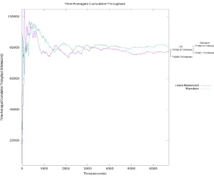
1. Time Averaged Cumulative Throughput
This experiment compares the time averaged cumulative throughput (given by Equation 3.1) under both the scenarios load balancing scheme and random path allocation. Be-cause under the traffic conditions simulated, it is almost impossible for any queue to be completely empty at any time, the time-averaged cumulative throughput is expected to be very similar for both cases. As depicted in Figure 3.3, the experiments done demonstrate that this conjecture is correct. Although the random path allocation scheme happens to perform slightly better than the load balancing algorithm over 30 runs of the simulation, there is not much to choose from between the two algorithms based solely on Time Av-eraged Cumulative Throughput.
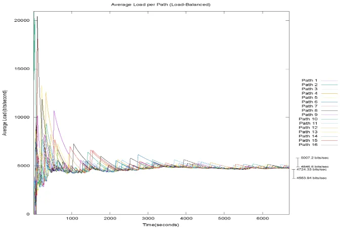
2. Time Averaged Load Per Path
been allocated to a path, it sticks to that path until it is completed, making the load on the concerned path relatively higher than the load on other paths. Similarly smaller flows can have the opposite effect which can affect minor imbalances between loads on each path.
3. Queue Lengths at Access and Distribution Layers
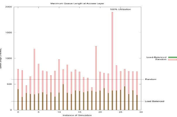
Described in this section are the group of experiments that clearly indicate the superiority of our Load Balancing scheme over a random path allocation scheme. Even though the time-averaged cumulative throughput results of both the algorithms do not have much to choose from, it is the behavior of queues that marks a clear distinction between the two algorithms. As part of the experiments, queue lengths were observed at the Access Layer and the Distribution Layer every time a new packet arrived at any of the switches at these layers. For each queue, the queue length was observed every time it changes and then the maximum queue length between time intervals of 10 seconds was selected for each scheme. Next the maximum queue length between these maximum values were picked up for each run of the simulation and plotted for 30 simulations. The results obtained clearly demonstrate that while the random path allocation algorithm has tremendous variation in queue lengths and has much higher buffer space requirements to accommodate its queues, the load balancing algorithm is far more predictable and has relatively lesser buffer space requirements to accommodate its queues at every switch.
As mentioned earlier, three sets of experiments were conducted at varying System Utilization of 100%, 90% and 80% respectively. Each set of experiments comprises the following results for both the path allocation schemes - Load Balanced and Random:
List of Experiments
1. Time averaged Cumulative Throughput over 30 simulations
2. Per Path Load over 30 simulations
3. Maximum Queue Lengths per simulation over 30 simulations at the Access Layer
System Utilization 100%
Time averaged Cumulative Throughput - Load Balanced Path Allocation vs Ran-dom Path Allocation
Figure 3.3: Cumulative Throughput - Load Balanced Path Allocation vs Random Path Allo-cation
Load-Balanced Path Allocation
Mean = 75524.16 bits/sec
Standard Deviation = 3544.64 bits/sec Confidence Interval (95%): ±1268.41 bits/sec
Range = 74255.76 bits/sec to 76792.57 bits/sec with a confidence of 95%
Random Path Allocation
Mean = 76386.50 bits/sec
Standard Deviation = 2791.11 bits/sec Confidence Interval (95%): ±998.77 bits/sec
Range = 75387.73 bits/sec to 77385.27 bits/sec with a confidence of 95%
Per Path Load - Load Balanced Path Allocation
Figure 3.4: Per Path Load - Load Balanced Path Allocation
beginning of the simulation, any path that is allocated to a flow will show a sudden spike in load as compared to the other paths because the average load recorded for this path is relatively very high as compared to the load recorded on all paths thus far. However, as the simulation moves in time, the impact of a flow allocation to a path and the sudden burst it brings in to the average load of that path is not as high as before when compared to the concurrent average load on the rest of the paths. So the spikes become less intense as the simulation moves in time. Further, the minimum and maximum final values of per Path Load over 30 simulations for the Load Balanced Path Allocation have been recorded. To elucidate, at the end of one run of the simulation, one path is bound to have the minimum load and another path is bound to have the maximum load between all possible paths. These minimum and maximum load values have been recorded for all the 30 simulations and the following observations have been made and also represented in Figure 3.4:
Load Balanced Path Allocation - Minimum Path Load
Mean = 4644.13 bits/sec
Standard Deviation = 224.10 bits/sec Confidence Interval (95%): ±80.19 bits/sec
Range = 4563.94 bits/sec to 4724.33 bits/sec with a confidence of 95%
Load Balanced Path Allocation - Maximum Path Load
Mean = 4926.90 bits/sec
Standard Deviation = 224.39 bits/sec Confidence Interval (95%): ±80.3 bits/sec
Range = 4846.6 bits/sec to 5007.20 bits/sec with a confidence of 95%
These results indicate that there is a 95% guarantee that the load on each path is going to be between about 4500 bits/second and 5000 bits/second no matter how many times the simulation is run, thus demonstrating that the load on all paths is similarly balanced.
Figure 3.5: Per Path Load - Random Path Allocation
Maximum Queue Lengths per Simulation over 30 simulations at the Access Layer
and Distribution Layer
Figure 3.7: Distribution Layer Queue Lengths at 100% System Utilization- Load Balanced Path Allocation vs Random Path Allocation
Figures 3.6 and 3.7 represent the maximum queue lengths observed for both the path allocation algorithms over 30 simulations at the Access layer and the Distribution layer respectively. These figures also demonstrate the advantage of using a dynamic Load Balancing algorithm such as the one described here. As explained before, the queue lengths are far more predictable for the Load Balancing scheme as compared to the Random Path Allocation scheme. Moreover, the queue length requirements are far less demanding for the Load Balancing scheme, thus allowing other concurrent applications besides content streaming to be able to use the surplus buffer space on the switches and servers.
System Utilization 90%
Figure 3.8: Access Layer Queue Lengths at 90% System Utilization- Load Balanced Path Allocation vs Random Path Allocation
System Utilization 80%
Figure 3.10: Access Layer Queue Lengths at 80% System Utilization- Load Balanced Path Allocation vs Random Path Allocation
As demonstrated by these results for Queue Lengths at Access Layer and Distribution Layer at different System Utilization, it is evident that our Load Balancing scheme outper-forms a Random Path Selection scheme for a variety of network traffic conditions. Finally, the maximum queue lengths observed at Access Layer and at Distribution Layer for both path selection schemes - Load Balancing and Random, were plotted against the System Utilization and it was observed that as System Utilization increases, the maximum queue length for our Load Balancing scheme remains more or less the same. On the other hand, the maximum queue lengths observed for Random Path Selection scheme increased rapidly with increasing System Utilization. The results were plotted in Figure 3.12 for the Access Layer and Figure 3.13 for the Distribution Layer and they summarize the advantage of our Load Balancing scheme over a Random Path Selection scheme with respect to queue lengths observed. They are presented below.
Figure 3.13: Distribution Layer Queue Lengths plotted against System Utilization- Load Bal-anced Path Allocation vs Random Path Allocation
3.3.4 Limitations of the Algorithm/Experimental Setup
Chapter 4
Conclusion and Future Work
This chapter summarizes the findings from the research and also dwells upon possible future work that can be done in this direction.
4.1
A Summary of Findings
Having simulated a Content Streaming Data Center environment, experiments were performed to analyze our Load Balancing algorithm with respect to Time-averaged Cumulative Through-put, Time-averaged Per Path Load and Queue Lengths observed in the switching fabric. Our scheme was contrasted with a Random Path Selection scheme and the results obtained were as
follows-1. Time-averaged Cumulative Throughput is very similar for Load Balancing scheme and Random Path Selection owing to the fact that Cumulative bits is going to increase at the same rate for both the schemes as long as all the queues have at least one packet to process throughout the course of the simulation.
2. The objective of balancing load between available paths was achieved with our algorithm.
3. Our Load Balancing Algorithm demonstrates far better queue length management as compared to a Random Path Selection Scheme.The surplus buffer space in switches can be used by other common data center applications such as MapReduce.
4.2
Future Work
1. The value ofαcan be experimented with and Load Balancing and Queuing behaviors can be observed. Customized Load Balancing Schemes can be built by using specific values of α for specific situations
2. The Load Balancing Algorithm can be extended to other popular data center topologies such as Clos topology.
REFERENCES
[1] Arregoces, M. and Portolani, M. (2004) Data Center Fundamentals Cisco Press, Indi-anapolis, IN.
[2] Benson, T., Akella, A. and Maltz, D.A. (2010) Network Traffic Characteristics of Data Centers in the WildIMC 2010, ACM SIGCOMM 2010 New York, NY
[3] Benson, T., Anand, A., Akella, A. and Zhang, M. (2010) Understanding Data Center Traffic CharacteristicsIMC 2010, ACM SIGCOMM 2010 New York, NY
[4] Torres, R., Finamore, A., Kim, J.R., Mellia, M., Munafo, M.M., and Rao, S. (2011) Dissecting Video Server Selection Strategies in the YouTube CDN ICDCS 2011, IEEE ICDCS 2011 Minneapolis, MN.
[5] Casado, M., and Pettit, J. (2013) Of Mice and Elephants Available at: http://networkheresy.com/2013/11/01/of-mice-and-elephants/
[6] Al-Fares, M., Radhakrishnan, S., Raghavan, B., Huang, N. and Vahdat, A. (2010) Hedera: Dynamic Flow Scheduling for Data Center NetworksNSDI 2010, 7th USENIX Conference, USENIX Association, Berkeley, CA
[7] Alizadeh, M., Edsall, T., Dharmapurikar, S., Vaidyanathan, R., Chu, K., Fingerhut, A., Lam, V.T., Matus, F, Pan, R., Yadav, N. and Varghese, G. (2010) CONGA: Distributed Congestion-Aware Load Balancing for DatacentersACM SIGCOMM 2014, New York, NY.
[8] Raiciu, C., Barre, S., Pluntke, C., Greenhalgh, A., Wischik, D., and Handley, M. (2011) Im-proving Data Center Performance and Robustness with Multipath TCPACM SIGCOMM 2011, New York, NY.
[10] Wang, R., Butnariu, D., and Rexford, J. (2011) OpenFlow-Based Server Load Balancing Gone WildHot-ICE 2011, 11th USENIX Conference, USENIX Association, Berkeley, CA
[11] Cisco Visual Networking Index: Forecast and Methodology, 2014-2019 White Paper (2015) Available at: http://goo.gl/ooPNri
[12] Kandula, S., Katabi, D., Sinha, S. and Berger, A. (2007)Dynamic Load Balancing Without Packet ReorderingACM SIGCOMM 2007, New York, NY.
[13] Internet Live Stats Available at: www.internetlivestats.com/one-second/
[14] Google Data Centers
Available at: http://www.google.com/about/datacenters/inside/locations/index.html
[15] Dent, S. (2015) Google Gives the World a Peek at its Secret Servers
Available at: http://www.engadget.com/2015/08/20/google-reveals-server-info/
[16] Google - Live Encoder Settings, Bitrates and Resolutions
Available at: https://support.google.com/youtube/answer/2853702?hl=en
[17] Inside YouTube Video Statistics - 2010
Available at: https://www.sysomos.com/reports/youtube-video-statistics