DOI: 10.1534/genetics.106.063743
Prediction of Breeding Values and Selection Responses With Genetic
Heterogeneity of Environmental Variance
H. A. Mulder,*
,1P. Bijma* and W. G. Hill
†*Animal Breeding and Genetics Group, Wageningen University, 6700 AH Wageningen, The Netherlands and
†Institute of Evolutionary Biology, School of Biological Sciences, University of Edinburgh,
Edinburgh EH9 3JT, United Kingdom Manuscript received July 21, 2006 Accepted for publication January 21, 2007
ABSTRACT
There is empirical evidence that genotypes differ not only in mean, but also in environmental variance of the traits they affect. Genetic heterogeneity of environmental variance may indicate genetic differences in environmental sensitivity. The aim of this study was to develop a general framework for prediction of breeding values and selection responses in mean and environmental variance with genetic heterogeneity of environmental variance. Both means and environmental variances were treated as heritable traits. Breeding values and selection responses were predicted with little bias using linear, quadratic, and cubic regression on individual phenotype or using linear regression on the mean and within-family variance of a group of relatives. A measure of heritability was proposed for environmental variance to standardize re-sults in the literature and to facilitate comparisons to ‘‘conventional’’ traits. Genetic heterogeneity of environmental variance can be considered as a trait with a low heritability. Although a large amount of information is necessary to accurately estimate breeding values for environmental variance, response in environmental variance can be substantial, even with mass selection. The methods developed allow use of the well-known selection index framework to evaluate breeding strategies and effects of natural selection that simultaneously change the mean and the variance.
T
HE standard genetic model in quantitative genetics is that phenotypePis the sum of genotypeGand environment E: P ¼G1E (Falconer and Mackay 1996). The phenotypic variance can be written ass2P¼
s2 G1s
2
E, assuming no covariance betweenGandE. This model allows for genetic differences in mean (G), with a genetic variance s2
G. For different genotypes, envi-ronmental variances (s2
E) are assumed to be constant. On the basis of analysis of field data and laboratory (selection) experiments, there is, however, some empir-ical evidence that genotypes differ ins2
E.
Several studies have been carried out to quantify genetic differences in environmental variance in field data. SanCristobal-Gaudyet al. (2001), Sorensenand Waagepetersen(2003), and Roset al. (2004) explicitly modeled genetic differences in environmental variance and found substantial genetic variance in environmen-tal variance for litter size in sheep, litter size in pigs, and body weight in snails, respectively. Van Vleck (1968) and Clayet al. (1979), in analysis of milk yield in dairy cattle, and Roweet al. (2006), in analysis of body weight in broiler chickens, found large differences between sires in phenotypic variance within progeny groups. In
these studies, it was not possible to distinguish whether these differences were due to heterogeneity of environ-mental variance, genetic variance, or both.
Several selection experiments have been carried out to investigate whether phenotypic variance can be changed by selection. Phenotypic variance changed in some se-lection experiments with Drosophila melanogaster and Tribolium castaneum(Rendel et al. 1966; Kaufmanet al. 1977; Cardinand Minvielle1986), while it did not in an experiment with mice (Falconerand Robertson1956). In these experiments, it was not always clear whether the response in variance was due to a change in environmen-tal variance, genetic variance, or both.
Mackay and Lyman (2005) derived 300 isofemale lines of Drosophila and computed the coefficient of variation (CV) for environmental variance within each homozygous line, effectively a clone, and within crosses of each line with another inbred line. They found highly significant genetic variance in the CV and in environ-mental variance between lines. Homozygotes had higher environmental variance, in agreement with findings of Robertsonand Reeve(1952). This study is probably the cleanest known example of showing genetic variance in environmental variance because the design allowed rep-etition of genotypes.
In livestock and plant breeding, uniformity of end product is an important topic. In meat type animals, for 1Corresponding author: Animal Breeding and Genetics Group,
Wageningen University, PO Box 338, 6700 AH Wageningen, The Netherlands. E-mail: herman.mulder@wur.nl
instance, uniformity has economic benefits because excessive variability in carcass weight or conformation is penalized by slaughterhouses. Hohenboken (1985) re-viewed the potential of mating systems (crossing, inbreed-ing) and breeding schemes to change variability. To evaluate breeding strategies, methods to predict responses to selection for uniformity are necessary. SanCristobal -Gaudy et al. (1998) derived prediction equations and SanCristobal-Gaudy et al. (2001) evaluated different selection indices using Monte Carlo simulation when the aim was to select for an optimum phenotype and thereby decrease the variance around the optimum (canalizing selection). Sorensenand Waagepetersen(2003) evalu-ated response to selection using an index including the mean and the variance of multiple records of an indi-vidual and Roset al. (2004) discussed the use of a re-stricted index aiming at decreasing the environmental variance, while maintaining the mean. Hilland Zhang (2004) derived simple equations to predict response to directional mass selection with genetic heterogeneity of environmental variance. In general, these prediction equations can be used only in special cases. A general framework to predict responses in mean and variance is lacking.
The objective of the present study was to develop a general framework for prediction of breeding values and responses to selection with genetic heterogeneity of environmental variance. Responses to selection were predicted for different forms of selection based on a single phenotype, as well as selection on a mean or var-iance of a group of relatives. Furthermore, a measure of heritability of environmental variance was developed, enabling a direct comparison between selection to change the environmental variance of a trait and the well es-tablished framework of selection to change its mean.
DERIVATION AND EVALUATION OF EXPRESSIONS
In this section, the model incorporating genetic heterogeneity of environmental variance is defined and the framework for prediction is explained. Pre-diction of breeding values and selection responses based on a single phenotype and a group of relatives are then considered, in each case using Monte Carlo simulation to investigate the relationships between true breeding values and phenotypic information. Using these obser-vations, multiple-regression equations are derived for one generation of selection and their goodness of fit is evaluated by simulation. Finally, a measure of heritability for environmental variance is proposed.
Genetic model and framework for prediction
The classical model, in the absence of dominance and epistasis,P ¼A1E (Falconerand Mackay 1996), is extended to include an additive genetic effect for the environmental variance,
P ¼m1Am1x
ffiffiffiffiffiffiffiffiffiffiffiffiffiffiffiffi
s2E1Av
q
ð1Þ
(Hilland Zhang2004), where mands2
Eare, respec-tively, the mean trait value and the mean environmental variance of the population,AmandAvare, respectively, the breeding value for the mean and environmental variance, and x is a standard normal deviate for the environmental effect. It is assumed thatAmandAv are the sum of the effects at an infinite number of loci each with small additive effects and follow a multivariate
normal distribution N 0
0 ;C5A
, where A is the
additive genetic relationship matrix,
C¼ s 2
Am covAmv
covAmv s
2
Av
" #
;
s2
Am is the additive genetic variance in Am, s 2
Av is the additive genetic variance inAv, covAmv¼covðAm;AvÞ ¼
rAsAmsAv, and rA is the additive genetic correlation betweenAmandAv. The termxis normally distributed
Nð0;1Þ and is scaled by ffiffiffiffiffiffiffiffiffiffiffiffiffiffiffiffis2 E1Av p
to obtain the environmental effect. The notation is listed in Table 1. The genetic model in Equation 1 does not allow for random environmental effects on the magnitude of the environmental variance, because without repeated measurements on each individual these cannot be separated from the usual random environmental ef-fects. With repeated measurements on each individual, these environmental effects on environmental variance become equivalent to permanent environmental effects (e.g., SanCristobal-Gaudyet al. 1998; Sorensen and Waagepetersen2003).
To predict the breeding values Aˆm and Aˆv and selection responsesDAm andDAv, multiple regression was used. Selection index theory is essentially an applica-tion of multiple regression (Hazel1943). Multiple regres-sion gives the best linear prediction (BLP), which is equal to best linear unbiased prediction (BLUP) when fixed effects are known without error (Henderson 1984). When variables are multivariate normally distributed, regressions are linear and homoscedastic (Lynch and Walsh 1998). Although the distribution of P deviates slightly from normality with genetic heterogeneity of envi-ronmental variance (s2
Av.0), P, Am, and Av follow an approximately multivariate normal distribution for values of s2
Av observed in the literature (e.g., S
anCristobal -Gaudyet al. 2001; Sorensenand Waagepetersen2003; Roset al. 2004; Rowe et al. 2006), justifying the use of multiple regression.
Multiple regression with selection on a single phenotype
withP, with the objective to decide which order of fit would be required for accurate prediction and then to evaluate the fit of predictions on the basis of multiple regressions. Fifty replicates with one phenotypic obser-vation on each of 500,000 unrelated animals in each rep-licate were generated according to the genetic model in Equation 1, assuming m¼0. The breeding valuesAm andAv and the environmental effectx were randomly drawn fromNð0;1Þand scaled by their corresponding standard deviations. When the genetic correlation be-tweenAmandAvwas nonzero,Avwas sampled given the expected value based onAmwith varianceð1rAÞ
2s2
Av. Expected breeding values were calculated as the mean Am and Av within successive intervals of 0.01 units of
P (s2
P¼1) and averaged over replicates. Expected selection responses to directional mass selection were calculated as the meanAmandAvof all selected animals havingP$xand averaged over replicates, wherexis the truncation point. The selected proportion was assumed to be the same in both sexes.
Breeding value estimation: Figure 1, A and B, pres-ents, respectively, the expectation ofAmgivenPand the expectation of Av given P2 when rA¼0, obtained by
simulation. These show that the relationship between Am and P is almost linear and that the relationship betweenAvandP2is also almost linear (quadratic inP). Therefore,P mroughly predictsAmand regression on
½P m2
Ef½P m2g
roughly predictsAv. As a conse-quence of genetic heterogeneity of environmental variance, the distribution of P is slightly leptokurtic and is slightly skewed whenrA6¼0. By fitting curves to
the simulation results, it was found that regression on
½P m3
Ef½P m3g
explained most of the residual nonlinearity and skewness whenrA6¼0. Moments ofPof
higher order did not improve the fit and were therefore not considered in the rest of this study.
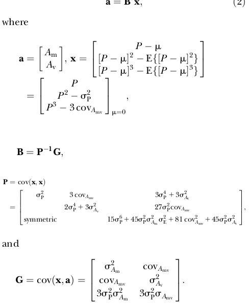
On the basis of this curve fitting, breeding values were predicted using multiple regression on the first through third order ofP,
ˆa¼B9x; ð2Þ
where
a¼ Am
Av
;x¼
P m
½Pm2Ef½P m2g ½Pm3Ef½P m3g
2 4
3 5
¼
P P2s2P
P33 covAmv
2 4
3 5
m¼0 ;
B¼P1G;
P¼covðx;xÞ ¼
s2
P 3 covAmv 3s
4 P13s
2
Av
2s4 P13s
2
Av 27s
2 PcovAmv
symmetric 15s6 P145s
2 Ps
2
Ams 2 E181 cov
2
Amv145s 2 Ps
2
Av 2
6 6 4
3 7 7 5;
and
G¼covðx;aÞ ¼ s2A
m covAmv
covAmv s
2
Av
3s2
Ps2Am 3s
2 PsAmv
2 6 4
3 7 5:
Elements of P and G were derived using the higher-order moments of the normal distribution (e.g., Stuart and Ord1994) and standard variance–covariance rules (see appendix a). Elements in these matrices were verified with Monte Carlo simulation.
TABLE 1
Notation used
P,m,Am,Av Phenotype, mean, breeding values for
mean and environmental variance x, MS Standard normal deviate, Mendelian
sampling term s2
Am,s
2
Av,rA,C Genetic variance in mean and
environmental variance, genetic correlation betweenAm andAv,
genetic variance–covariance matrix s2
E,s 2
P Mean environmental and phenotypic
variances Ps,Ps2,Ps3 MeanP,P
2, andP3of selected animals
P,ðPÞ2
,P2,n Mean phenotype of relatives, mean
phenotype squared, mean squared phenotype of relatives, number of relatives
varW, lnðvarWÞ Within-family variance, log-transformed within-family variance
aj,aw Additive genetic relationships
between animaljand the group of relatives and between animals within the group of relatives
a,x Vectors of breeding valuesAmand
Av and of phenotypic information P,G,gAm,gAv Variance–covariance matrix ofx,
covariance matrix betweenxanda, vectors withG¼ ½gAm gAv Pln,Gln,L P- andG-matrices with lnðvarWÞ,
scalar matrix
B,bAm,bAv Matrix with regression coefficients,
vectors withB¼ ½bAm bAv
i,x,p,z Selection intensity, truncation point, selected proportion, ordinate of standard normal distribution DAm,DAv,rAˆv;Av Response inAm andAv, accuracy ofAˆv
h2 m,h
2
v, GCVE Heritability of mean and
environmental variance, evolvability of environmental variance
s2
E;exp,Av;exp,s2Av;exp Environmental variance, breeding
Evaluation of predictions: Predictions of Equation 2 were close to the expectations obtained from Monte Carlo simulation when rA¼0, as could be expected
from the almost linear relationships shown in Figure 1, A and B (R2.0:98). Forr
A¼0:5, Figure 2A shows that Am is approximately linear inP, with a slope close to
h2 m¼s
2
Am= s 2
Am1s 2 E
¼0:3, for Pwithin two standard deviations (SD) of its mean, but becomes curvilinear for extremeP. The predictedAmusing the full model with multiple regressions onP,P2, andP3fitted well to the
expectations obtained from Monte Carlo simulation (R2.0:99) and, in contrast to multiple regressions on onlyP and P2, also explained the nonlinearity in the
extremes.
Figure 2B shows that the relationship between Av andP is highly curvilinear forrA¼0:5, with higherAv for more extremeP. As forAˆm, the predictedAv using the full model with multiple regressions onP,P2, andP3
fitted well to the expectation from Monte Carlo simu-lation (R2.0:99). The use of only P and P2 was
ad-equate only within 2 SD of the mean, but was biased for extremeP.
Response to mass selection: Response to selection (DG) is predicted asDG ¼bS, wherebis the regression coefficient of the breeding value on the selection criterion, andSis the selection differential in units of the selection criterion (e.g., phenotype) (Falconerand Mackay1996). With homogenous environmental vari-ance and directional mass selection,b¼h2andS¼is
P,
whereiis the selection intensity, andDG ¼ih2
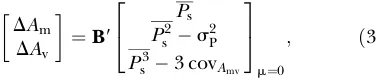
mspis the breeders’ equation (Falconer and Mackay 1996; Lynchand Walsh 1998). With genetic heterogeneity of environmental variance, directional mass selection leads to responses in mean and variance (Hill and Zhang 2004). To predict this, Equation 2 can be rewritten asDa¼B9Dx, giving
DAm DAv
¼B9
Ps
Ps2s2 P
Ps33 covAmv
2 4
3 5
m¼0
; ð3Þ
where Ps,Ps2, andPs3 are the respective means for the selected animals.
Directional selection: With directional selection by truncation,Ps¼isP, wherei¼z=pfor normally distrib-uted observations, z is the height of the standardized normal at the truncation pointx, andpis the selected proportion (Falconerand Mackay1996; Lynchand Walsh1998).P2
s andPs3were calculated by integration assuming that P is normally distributed, which is approximately the case for observed values of s2
Av in the literature:
Ps2 ¼ ðix11Þs2
P ð4aÞ
Ps3 ¼ ðix212iÞs3
P: ð4bÞ
Figure 2.—Expected (MC) and predicted
breeding valuesAm(A) andAv(B) based on a
sin-gle phenotype as a function of phenotype using the full model with multiple regression onP,P2,
andP3(MR3) or the reduced model with multiple
regression onPandP2(MR2) (s2
Am¼0:3;s
2 Av¼0:05;
rA¼0:5;s2E¼0:7;s 2 P¼s
2
Am1s
2 E¼1:0).
Figure 1.—ExpectedA
m (A) andAv (B) as a
function of P and P2, respectively (s2 Am¼0:3;
s2
Av¼0:05; rA¼0; s
2
E¼0:7; s2P¼s2Am1s
2 E¼
The predicted response to directional mass selection is thus
DAm DAv
¼B9
isP
ixs2P ðix212iÞs3
P3 covAmv
2 4
3
5: ð5Þ
The term P2
s s2P¼ixs2P is similar to the term 12ixs2P derived by Hill and Zhang (2004), who calculated the probability of selection by using a Taylor series approximation, where the factor1
2appears here in the B-matrix, assuming thatrA¼0 ands2Av is small. Equa-tion 5 can be rewritten using the regression coefficients inB and ignoring the terms involvingP3, which were
not included by Hilland Zhang(2004),
DAm¼ s2A
mð2s
4 P13s
2
AvÞ 3 cov
2
Amv
D isP
1ðs 2
P3s2AmÞcovAmv
D ixs
2
P ð6Þ
DAv¼
2s4 PcovAmv
D isP1
s2Ps2A
v3 cov
2
Amv
D ixs
2
P; ð7Þ
where D¼detðPÞ ¼s2 Pð2s
4 P13s
2
AvÞ 9 cov 2
Amv. When
s2
AvandrAare close to zero, Equations 6 and 7 approach
DAm¼ ðs2Am=s 2
PÞisP and DAv¼ ðs2Av=2s 4 PÞixs
2
P, which are Equations 10 and 11 of Hill and Zhang(2004). Differences arise whenrAis substantially different from
zero, as the covariance betweenP andP2was ignored
by Hill and Zhang.
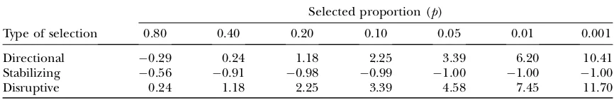
Stabilizing and disruptive selection: Stabilizing and disruptive selection can be considered as selecting the animals with low or highP2, respectively (Falconerand Mackay1996). Assuming that selection is by truncation, selection differentialsP2
s for P2can be obtained from Equation 4a and selection differentials forPandP3are
zero for these types of selection whenPis normally dis-tributed. With stabilizing selection by truncation, ani-mals only in the middle of the distribution are selected, giving a selection differential
Ps2¼h1 2p*i*x*=ð12p*Þis2P; ð8aÞ
wherei* andx* are, respectively, the selection intensity and truncation point corresponding top*¼1
2ð1pÞ,
the proportion of animals culled on one side of the distribution. With disruptive selection by truncation, the extreme animals in both tails of the distribution are selected, giving a selection differential
Ps2 ¼ ði*x*11Þs2
P; ð8bÞ
wherep*¼1
2p, the proportion of animals selected on
one side of the distribution. The standardized selection differentials P2
s s2P for directional, stabilizing, and disruptive selection are in Table 2.
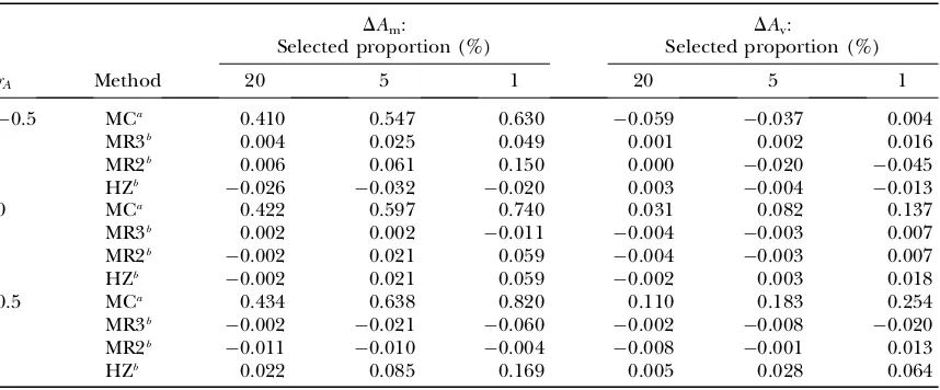
Evaluation of predictions with directional mass selection: The predictions of Equation 5 [multiple regressions (MR) 3] and Equations 6 and 7 (MR2) and those of the Hill–Zhang (HZ) model (Hill and Zhang2004) are compared in Table 3 with the observed responses ob-tained from Monte Carlo (MC) simulation, for different values of rA and selected proportions. Multiple
regres-sions on P, P2, andP3(MR3) predicted the responses
well, with prediction errors ,5% when the selected proportion was at least 5% (prediction error relative to
DAm with s2Av ¼0:05, rA¼0, p¼0:05). Prediction errors were on average smaller for MR3 than for MR2, although occasionally larger. They were also on average slightly smaller for MR2 than for the Hill–Zhang model, especially with rA¼0:5, because in the latter the
co-variance between P and P2 was not accounted for in
calculation of the regression coefficients. Prediction errors using MR were mainly due to poor prediction of selection differentials because of deviations from nor-mality and thus increased with decreasing selected pro-portion as the tails of the distribution were most affected (results not shown). Whens2
Avincreased to 0.10 or 0.15, which reflects the upper range of estimates in the literature (e.g., SanCristobal-Gaudy et al. 2001; Ros et al. 2004), prediction errors increased up to 10–20% (prediction error relative to DAm with s2Av ¼0:05,
rA¼0, p ¼0:05), especially with selected proportion
of 1% (results not shown). Increasing s2
Av increases deviations from normality in P, but it seems that the multiple-regression framework is robust against these relatively small deviations from normality, except when the selected proportion is very small. It can be con-cluded that MR3 is the preferred method for predicting responses inAmandAvwith directional mass selection, TABLE 2
Standardized selection differentials ofP2
sfor directional, stabilizing, and disruptive selection by truncation on a
normal distribution corrected for the expectation ofP2(¼1) for different selected proportions (p)
Selected proportion (p)
Type of selection 0.80 0.40 0.20 0.10 0.05 0.01 0.001
Directional 0.29 0.24 1.18 2.25 3.39 6.20 10.41
Stabilizing 0.56 0.91 0.98 0.99 1.00 1.00 1.00
having prediction errors ,5% when at least 5% are selected.
Multiple regression with selection based on a group of relatives
Monte Carlo simulation:In animal breeding sires are often selected on performance of their half-sib progeny. Monte Carlo simulation was used to investigate relation-ships between theAmandAvof the sires and statistics on phenotypes of their progeny and then to evaluate the fit of predictions on the basis of multiple regressions. Fifty replicates were generated of 500,000 unrelated sires each with 10 or 100 half-sib progeny or of 50,000 un-related sires each with 1000 or 10,000 half-sib progeny. Data were simulated according to the genetic model in Equation 1. The breeding values of sires (As;mandAs;v) and unrelated random-mated dams (Ad;mandAd;v) were randomly sampled with variances2
Amors 2
Av, respectively. For each progeny, the Mendelian sampling terms MSm and MSvwere randomly sampled with variance12s2Amand
1 2s
2
Av, respectively, to give breeding values for each progeny (Ap;mandAp;v):
Ap¼
1 2As1
1
2Ad1MS:
When the genetic correlation betweenAm andAv was nonzero, breeding valuesAv and Mendelian sampling terms MSv were sampled given their expected value based on Amor MSmand with varianceð1rAÞ
2s2
Av or
1
2ð1rAÞ
2s2
Av, respectively. For each progeny, the envi-ronmental effect x was randomly sampled and scaled with its standard deviation.
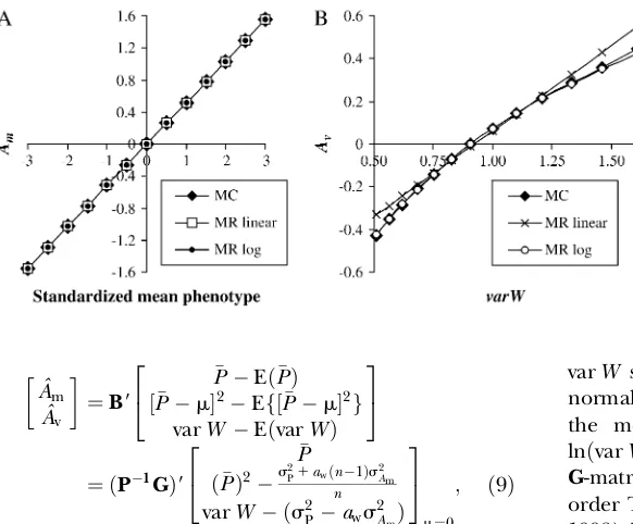
Expected breeding values of sires were calculated as the meanAmandAv within successive intervals of 0.01 SD units of progeny meanP or log-transformed within-family variance [lnðvarWÞ] and averaged over replicates. Expected genetic selection differentials of directional selection onPwere calculated as the meanAmandAvof all selected sires with ðP=sPÞ$x and averaged over replicates.
Breeding value estimation: When there is an obser-vation on only a single phenotype, there is no indepen-dent information available on the mean and variance of the genotype, although P and P2 provide point
esti-mates. When phenotypes of a group of relatives each having the same relationship to an individual are avail-able (e.g., progeny), statistics such asP,ðPÞ2
, and varW can be used to predict itsAmandAv. HerePis the mean phenotype and P2 is the mean P2 of the relatives,
varW ¼ ½n=n1ðP2 ðPÞ2Þ is the within-family vari-ance, andnis the number of relatives within the group. With largen, varW becomes the main predictor ofAv, but otherwise ðPÞ2 contains additional information because animals with a highAvhave a higher probability of having a very high or low P. This is similar to directional mass selection and the termðPÞ2therefore plays an equivalent role toP2. Although the Monte Carlo
simulation was based on sires with half-sib progeny, the prediction of breeding values generalizes to any group of relatives with the same relationship. The multiple-regression equation can be represented as
TABLE 3
Response to directional mass selection inAm(DAm) andAv(DAv) for different valuesrAand selected
proportions comparing predictions [as prediction errors (predicted minus observed)] with observed responses obtained from Monte Carlo simulation (MC)
DAm: DAv:
Selected proportion (%) Selected proportion (%)
rA Method 20 5 1 20 5 1
0.5 MCa 0.410 0.547 0.630 0.059 0.037 0.004
MR3b 0.004 0.025 0.049 0.001 0.002 0.016
MR2b 0.006 0.061 0.150 0.000 0.020 0.045
HZb 0.026 0.032 0.020 0.003 0.004 0.013
0 MCa 0.422 0.597 0.740 0.031 0.082 0.137
MR3b 0.002 0.002 0.011 0.004 0.003 0.007
MR2b 0.002 0.021 0.059 0.004 0.003 0.007
HZb 0.002 0.021 0.059 0.002 0.003 0.018
0.5 MCa 0.434 0.638 0.820 0.110 0.183 0.254
MR3b 0.002 0.021 0.060 0.002 0.008 0.020 MR2b 0.011 0.010 0.004 0.008 0.001 0.013
HZb 0.022 0.085 0.169 0.005 0.028 0.064
a
Observed responses obtained from MC simulation:s2
Am¼0:3;s
2
Av¼0:05;s
2
E¼0:7;s 2 P¼s
2
Am1s
2 E¼1:0.
b
Predictions: MR3, multiple regressions onP,P2, andP3(see Equation 5); MR2, multiple regressions onPand
ˆ Am
ˆ Av
¼B9
PEðPÞ
½Pm2Ef½
P m2g
varW EðvarWÞ
2 4
3 5
¼ ðP1GÞ9
P
ðPÞ2s2P1awðn1Þs2Am
n varW ðs2
Paws2AmÞ
2 4
3 5
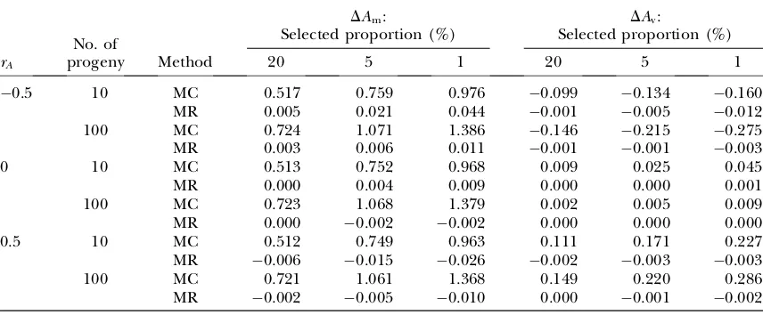
m¼0 ; ð9Þ
where aw is the additive genetic relationship between relatives within the family,
P¼
ðs2
P1awðn1Þs2AmÞ=n ½f313awðn1ÞgcovAmv=n 2
2½ðs2P1awðn1Þs2AmÞ=n 2
1ð½f313awðn1Þgs2Av=n 3Þ
symmetric
2 6 6 6 6 6 6 4
½f31awðn3ÞgcovAmv=n
½f31awðn3Þgs2Av=n 2
2ðs2
Paws2AmÞ 2
h i
=ðn1Þ
1 ½f3ðn1Þ1awðn
22n13Þgs2
Av
ðnðn1ÞÞ
! 3 7 7 7 7 7 7 5 ;
G¼
ajs2Am ajcovAmv
ajcovAmv=n ajs 2
Av=n
ajcovAmv ajs 2
Av 2
6 4
3 7 5;
and aj is the relationship of relatives to individual j.
Elements in theP- andG-matrices, derived inappendix a, were verified with Monte Carlo simulation for the case
of sires with half-sib progeny.
Log-transformation of var W: In multiple regression linearity is assumed and is typically satisfied if the explan-atory variables are normally distributed. Because variances of normally distributed variates arex2- distributed, the dis-tribution of varW is not normal. As the number of relatives increases, varW approaches a normal distribu-tion, but the convergence is slow (Stuartand Ord1994). The relationship between Av and varW is therefore nonlinear if there are a finite number of relatives (see Figure 3B), and also the sampling variance of varW increases with its mean. A logarithmic transformation of
varW seems a logical choice to reduce both the non-normality of varW and the positive relationship between the mean and its sampling variance. When using lnðvarWÞinstead of varW, the elements in the P- and
G-matrices involving varWwere transformed using a first-order Taylor series approximation (Lynchand Walsh 1998). The matricesPlnandGlninvolving lnðvarWÞwere calculated, respectively, as Pln¼LPL and Gln¼LG, whereL¼diagð1;1;1=varWÞwith 1=varW based on a first-order Taylor series approximation. The quantity EðlnðvarWÞÞwas calculated using a second-order Taylor series approximation (Lynch and Walsh 1998): EðlnðvarWÞÞ ¼lnðvarWÞ ðs2
varW=2varW
2
Þ, replacing EðvarWÞin Equation 9.
Evaluation of predictions: Predictions of Equation 9, which holds for any group of relatives with the same relationship, were evaluated for the case of sires with half-sib progeny. The expected and predicted values ofAmare shown as a function of the standardizedPof 100 half-sib progeny in Figure 3A forrA¼0.Amis linear in standard-ized P with a slope of 1
2s
2
Am=
ffiffiffiffiffiffiffiffiffiffiffiffiffiffiffiffiffiffiffiffiffiffiffiffiffiffiffiffiffiffiffiffiffiffiffiffiffiffiffiffiffiffiffiffiffi
s2
P114ðn1Þs
2
Am
=n q
¼
0:517. The predictedAˆmfitted well the expectation from Monte Carlo simulation (R2.0:99) and the predictions using varW or lnðvarWÞdid not differ ifrA¼0.
Figure 3B shows that the relationship betweenAvand varW is curvilinear for the case of 100 half-sib progeny when rA¼0. The predicted Av using untransformed varW(MR linear) overestimatedAvfor extreme values of varW, whereas predictedAvusing log-transformed varW (MR log) was curvilinear in varW and fitted well the expectation from Monte Carlo simulation (R2.0:99).
As the bias inAˆv was largest with extreme values of varW, the bias inAˆv at 2 SD from the mean lnðvarWÞ predicted by multiple regression using either varW or lnðvarWÞwas computed for different values ofs2
Av and numbers of progeny per sire (Table 4). Multiple regres-sion on varWwas seen to overestimate, but on lnðvarWÞ
to underestimate,Aˆv. The bias using lnðvarWÞwas neg-ligible when the number of progeny was 100, but increased when the number of progeny was small (10) or large (10,000). The bias with varWwas negligible with 10,000 progeny, as could be expected from the slow
Figure3.—Expected (MC) and predictedAm
as a function of the standardized mean pheno-type of half-sib progeny (A) and expected and predictedAvas a function of varW (B) using
ei-ther varW (MR linear) or lnðvarWÞ(MR log) in multiple regression (s2
Am¼0:3; s
2
Av¼0:05;
rA¼0; s2E¼0:7; s2P¼s2Am1s
2
E¼1:0; number
convergence of ax2-distribution to a normal distribu-tion, and was small with a few progeny. Note that a higher degree of symmetry between the expectedAvat2 and 2 SD of the mean lnðvarWÞcorresponded with a smaller bias inAˆvwith lnðvarWÞ. The value of log-transformation of varWthus depends on the number of progeny per sire.
Response to directional selection on family mean:
With the common procedure in livestock breeding to directionally select animals by truncation on the mean (P) of relatives,e.g., progeny, information on the within-family variance (varW) is ignored. As for mass selection, if there is genetic heterogeneity of environmental variance, animals with a higherAv would have a higher probability of selection when the selected proportion is
,50%, diminishing as the number of relatives increases. If Am and Av are uncorrelated, the response in Av is proportional to the selection differentialðPÞ2
s,
DAv ¼b½ðPÞ2s EfðPÞ2g ¼bixvarðPÞ; ð10Þ
where
b¼covðAv;j;ðPÞ
2Þ
varðPÞ2
¼ ajn
2s2
Av
2ns4
P14awnðn1Þs2Ps 2
Am12a 2 wnðn1Þ
2s4
Am1ð313awðn1ÞÞs 2
Av
lim n/‘b¼
ajs2Av
2a2 wns4Am
¼0: ð11Þ
There is therefore no selection pressure onAv with an infinite number of relatives (Equation 11), as suggested by Hilland Zhang(2004) using a different argument.
Response in Am andAv with selection onP can be generalized as
DAm DAv
¼B9 Psm ðPsÞ2varðPÞ
m¼0
¼B9 isP ixs2P
: ð12Þ
To compute (12), varW was not included in the in-formation vectorxbecause selection is solely onP. For infinitely many relatives, Equation 12 can be rewritten as
DAm¼ajisAm=
ffiffiffiffiffi aw
p
, which is the corresponding stan-dard breeders’ equation, andDAv ¼ajirAsAv=
ffiffiffiffiffi aw
p
, show-ing that response inAvthen becomes solely a correlated response to selection onP.
Evaluation of predictions: Table 5 shows predicted responses (Equation 12) inAm andAv when selecting on the mean of half-sib progeny (P) in comparison to observed responses from Monte Carlo simulation. In general, these agreed well, although prediction errors were slightly higher when rA6¼0, especially with high
selection intensity. As expected, the response in Am increased with more progeny (higher accuracy of se-lection) and lower selected proportion (higher selec-tion intensity). The response inAvwas small, becoming negligible with 100 progeny/sire whenrA¼0, but was,
however, substantial when rA6¼0, basically as a
corre-lated response to selection on the mean. Response inAv increased nonlinearly with increasing selection inten-sity, similar to directional mass selection, but to a lesser extent. In conclusion, responses in Am and Av to se-lection onPcan be predicted accurately using multiple regression.
TABLE 4
The expectation ofAvand bias inAˆvat lnðvar WÞ6xslnðvar WÞusing either varWor ln(varW) in multiple
regression for different values ofs2
Av and numbers of half-sib progeny per sire
x(¼lnðvarWÞ6xslnðvarWÞ)
Bias inAˆv (¼AvAˆv)
EðAvÞ varW lnðvarWÞ
s2
Av No. of progeny 2 2 2 2 2 2
0.01 10 0.016 0.032 0.001 0.000 0.007 0.009
100 0.066 0.076 0.004 0.003 0.004 0.005
1,000 0.155 0.155 0.009 0.007 0.001 0.001 10,000 0.187 0.198 0.001 0.004 0.007 0.004
0.05 10 0.084 0.133 0.011 0.018 0.024 0.025
100 0.286 0.283 0.042 0.042 0.003 0.000 1,000 0.392 0.436 0.014 0.023 0.025 0.018 10,000 0.407 0.484 0.002 0.002 0.037 0.040
0.10 10 0.173 0.234 0.039 0.054 0.030 0.031
100 0.467 0.475 0.072 0.081 0.005 0.004
1,000 0.556 0.658 0.025 0.035 0.053 0.049 10,000 0.569 0.710 0.017 0.004 0.060 0.080
s2
Am¼0:3;rA¼0;s
2
E¼0:7;s2P¼s2Am1s
Defining a measure of heritability for environmental variance at the phenotypic level
Heritability (h2¼s2
A=s
2
P) is a central parameter in quantitative genetics (Falconer and Mackay 1996; Lynchand Walsh1998). For standardization of results of analysis of genetic heterogeneity of environmental heterogeneity in field data and for making comparisons to ‘‘conventional’’ traits easier, it would be helpful to define a measure of heritability (h2
v) for environmental variance at the phenotypic level. Heritability equals the regression coefficient of the breeding value A on the phenotypeP. Here we propose a definition ofh2
v, which equals the genetic variance in environmental variance as a proportion of the variance of P2. This
definition is equal to the regression ofAv onP2, where
b¼covðAv;P2Þ=varðP2Þ ¼s2Av=varðP
2Þ and varðP2Þ ¼ 2s4
P13s 2
Av, andh 2
v is therefore
h2v ¼ s 2
Av
2s4 P13s2Av
: ð13Þ
Alternatively, h2
v could be defined at the level of environmental variance, which equals one in Equation 1. On the basis of single phenotypic records, the envi-ronmental variance of a genotype is, however, not es-timable. The measure of heritability in Equation 13 is directly related to single squared phenotypic records and as such is the natural analogy of the classical heritability of the mean (h2
m), which can be used in pre-diction of response to mass selection whenrA¼0.
Under the assumption ofs2
Am ¼0 and making use of Equation 13, Equation 9 can be greatly simplified when selecting on information of a group of relatives, for
example, half-sib progeny. When s2
Am ¼0, varW re-duces toðn=n1ÞP2becauseEðPÞ ¼0, so the multiple regression forAˆv can be simplified by regressing solely onP2. The accuracy ofAˆ
v can then be derived as
rAˆv;Av ¼
ffiffiffiffiffiffiffiffiffiffiffiffiffiffiffi
bAv9gAv
p
sAv
¼ 1 sAv
ffiffiffiffiffiffiffiffiffiffiffiffiffiffiffiffiffiffiffiffiffiffiffiffiffiffiffiffiffiffiffiffiffiffiffiffiffiffiffiffiffiffiffiffiffiffiffiffiffiffiffiffiffiffiffiffiffiffiffiffiffiffiffiffiffiffiffiffiffiffiffiffiffiffiffiffiffi
ð1=2Þns2A
v
2s4P13s2A
v1ð1=4Þðn1Þs
2
Av
31
2s
2
Av
s
¼
ffiffiffiffiffiffiffiffiffiffiffiffiffiffiffiffiffiffiffiffiffiffiffiffiffiffiffiffiffiffiffiffiffiffiffiffiffiffiffiffiffi
ð1=4Þnh2v 11ð1=4Þðn1Þhv2; s
ð14Þ
wherebAv andgAv are columns ofBandG correspond-ing toAv. The resulting expression is exactly the same as that for accuracy ofAm(Cameron1997), except thath2 is replaced by h2
v. To investigate the effect of assuming
s2
Am ¼0, the accuracy ofAˆvpredicted with Equation 14 was compared to that predicted using Equation 9 and Monte Carlo simulation whenrA¼0 (Table 6). In
gen-eral, accuracies were slightly underestimated by Equa-tion 14, increasingly so with greaters2
Am(s 2
P¼1), whereas the ones of Equation 9 were close to those from simula-tion. It seems thath2
v can be used as a first approxima-tion in standard predicapproxima-tion equaapproxima-tions when rA¼0,
but predictions should be interpreted with caution.
EXAMPLES OF CHANGING ENVIRONMENTAL VARIANCE BY SELECTION
In the previous section the focus was mainly on evaluating the goodness of fit of multiple-regression predictions with Monte Carlo simulation, but the results TABLE 5
Response to selection on mean of half-sib progeny (P) inAm(DAm) andAv(DAv) for different values of
rA, different numbers of progeny/sire, and different selected proportions comparing predictions (MR)
[as prediction errors (predicted minus observed)] with observed responses obtained from Monte Carlo simulation (MC)
DAm: DAv:
Selected proportion (%) Selected proportion (%)
rA
No. of
progeny Method 20 5 1 20 5 1
0.5 10 MC 0.517 0.759 0.976 0.099 0.134 0.160
MR 0.005 0.021 0.044 0.001 0.005 0.012
100 MC 0.724 1.071 1.386 0.146 0.215 0.275
MR 0.003 0.006 0.011 0.001 0.001 0.003
0 10 MC 0.513 0.752 0.968 0.009 0.025 0.045
MR 0.000 0.004 0.009 0.000 0.000 0.001
100 MC 0.723 1.068 1.379 0.002 0.005 0.009
MR 0.000 0.002 0.002 0.000 0.000 0.000
0.5 10 MC 0.512 0.749 0.963 0.111 0.171 0.227
MR 0.006 0.015 0.026 0.002 0.003 0.003
100 MC 0.721 1.061 1.368 0.149 0.220 0.286
MR 0.002 0.005 0.010 0.000 0.001 0.002
s2
Am¼0:3;s
2
Av ¼0:05;s
2
E¼0:7;s2P¼s2Am1s
also show the effects of selection on environmental variance. For example, the response inAv with direc-tional mass selection increased nonlinearly with increas-ing selection intensity (Table 3), and environmental variance increased unlessrA,0. The response inAvwas, however, negligible with directional selection on a half-sib progeny mean when rA¼0 (Table 5), but was
substantial whenrA6¼0, due to a correlated response.
We now use the formulas (Equations 2, 3, and 9) to assess the effects of selection strategies aimed at changing the environmental variance, taking values of
s2
Avbetween 0.01 and 0.10. These correspond to a lowh 2 v but are large relative tos2
E¼0:7, indicating a genetic coefficient of variation between 14 and 45%, higher than that for standard quantitative traits (Houle1992). As expected, the accuracy of Aˆv increased with s2Av (Table 7). The accuracy was low when using information only on own phenotype or a small number of progeny, but increased with number of relatives, especially with half-sib progeny, and when rA6¼0. With 1000 half-sib
progeny, the accuracy was.0.90, unlesss2
Av ¼0:01.
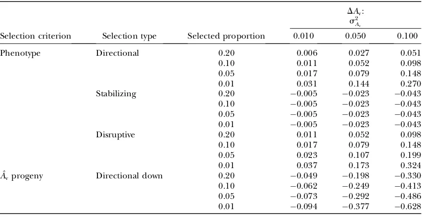
Table 8 shows the predicted response in Av for directional, stabilizing, and disruptive selection based on phenotype (Equation 3, selection differentials from Table 2, neglecting the terms involving P3) and for
directional downward selection onAˆvbased on 100 half-sib progeny assuming rA¼0 [calculated as DAv¼
irAˆv;AvsAv, where rAˆv;Av ¼
ffiffiffiffiffiffiffiffiffiffiffiffiffiffiffi
bAv9gAv
p
=sAv). Predictions were close to observed responses in Monte Carlo simulation. For all selection strategies, responses inAv increased withs2
Avdue to a higher accuracy and a higher genetic variance in itself.
With directional and disruptive selection on pheno-type, the predicted response in Av was positive and environmental variance increased substantially and non-linearly with selection intensity. Disruptive selection gave a slightly larger response because the selection intensity in each tail of the distribution of P was higher. With stabilizing selection on phenotype, the response inAvwas negative but small, even when the selection was intense because selection differentials remain small and were nearly constant (Table 2). With directional downward TABLE 6
Realized (MC) and predicted accuracy ofAˆvfor different numbers of half-sib progeny per sire ands2Amusing
either the exact prediction (MR exact) or the approximate prediction (MR approx)
No. of progeny
10 100
s2
Am MC MR exact MR approx MC MR exact MR approx
AccuracyAˆv
0 0.235 0.235 0.235 0.607 0.607 0.607
0.1 0.236 0.236 0.235 0.615 0.615 0.607
0.3 0.243 0.244 0.235 0.633 0.633 0.607
0.6 0.251 0.260 0.235 0.648 0.663 0.607
The exact prediction with multiple regression:rAˆv;Av¼
ffiffiffiffiffiffiffiffiffiffiffiffiffiffiffi bAv9gAv p
=sAv, wherebAv and gAv are columns ofB
andG. The approximate prediction (Equation 14):rAˆv;Av¼
ffiffiffiffiffiffiffiffiffiffiffiffiffiffiffiffiffiffiffiffiffiffiffiffiffiffiffiffiffiffiffiffiffiffiffiffiffiffiffiffiffiffiffiffiffi 1
4nhv2=ð1114ðn1Þhv2Þ q
, whereh2
v ¼s2Av=ð2s
4 P13s2AvÞ
and with assumptions2
Am¼0.s
2
Av ¼0:05;rA¼0;s
2
E¼1s2Am;s
2
P¼s2Am1s
2 E¼1:0.
TABLE 7
Predicted accuracy ofAˆvbased on a single phenotype or different numbers of full-sibs or half-sib progeny
for different values ofs2
Av andrA
rA¼0: rA¼0:5:
s2
Av s
2 Av
Information No. of progeny 0.01 0.05 0.10 0.01 0.05 0.10
Predicted accuracyAˆv
Phenotype — 0.070 0.152 0.209 0.279 0.299 0.319
Full-sibs 10 0.123 0.252 0.327 0.299 0.348 0.388
50 0.267 0.468 0.544 0.394 0.505 0.560
100 0.355 0.553 0.610 0.442 0.570 0.617
Half-sib 10 0.115 0.244 0.325 0.346 0.386 0.424
Progeny 50 0.257 0.499 0.618 0.490 0.597 0.671
100 0.353 0.633 0.745 0.545 0.693 0.772 1000 0.768 0.933 0.962 0.798 0.936 0.963
s2
Am¼0:3;s
2
E¼0:7;s 2 P¼s
2
Am1s
selection onAˆvbased on 100 half-sib progeny, response in
Av was negative and environmental variance decreased substantially, which in an agricultural context would imply increased uniformity of end product. Responses increased linearly with selection intensity and became large, especially withs2
Av$0:05. When the best 5% of the sires are selected onAˆvand dams are selected at random with s2
Av ¼0:05, the environmental variance would be 0.554 in the next generation, which is only 79.1% of that in the current generation! In conclusion, a large number of progeny is necessary to predictAˆv with high accuracy, but responses inAv can be large relative to the environ-mental variance in the current generation.
DISCUSSION
A multiple-regression framework has been developed to predict breeding values and selection responses in mean and variance for mass selection and selection between families in the presence of genetic heteroge-neity of environmental variance. The model of Hilland Zhang (2004) has been refined for directional mass selection and extended to stabilizing and disruptive selection based on phenotype and to between-family se-lection. The phenotypic variance increases nonlinearly with selection intensity under directional mass selection whenrA¼0. It increases even more with disruptive
tion, but decreases only slightly with stabilizing selec-tion, which is in agreement with results of Gavrilets and Hastings(1994) and Wagneret al. (1997). With selection on family mean, phenotypic variance is
ex-pected to change little unless rA6¼0, but with
selec-tion on within-family variance, response in phenotypic variance may be large providing s2
Av.0, even though a large number of relatives is necessary to estimateAˆv accurately.
Methodology: Comparison of genetic models: Different genetic models to account for genetic heterogeneity of environmental variance appear in the literature, basi-cally either additive effects both at the level of the mean and at the level of the environmental variance (Hill and Zhang2004; Zhangand Hill2005; this study) or additive effects on the mean and an exponential model for the environmental variance (SanCristobal-Gaudy et al. 1998, 2001; Sorensenand Waagepetersen2003; Roset al. 2004). In the exponential model
P ¼m1Am1xexp
lnðs2
E;expÞ1Av;exp
2
!
; ð15Þ
where s2
E;exp is the environmental variance when
Av;exp¼0, andAv;expis the individual’s breeding value for environmental variance in the exponential model, such that environmental variances are multiplicative on the observed scale and additive on a log-scale. (Note that lnðs2
E;expÞ ¼h in the notation of SanCristobal -Gaudy et al. 1998.) The distribution of true variances (not variance estimates) is unknown in practice and cannot help in guiding whether the additive model or the exponential model better reflects the real world. Clearly, each model has specific (dis)advantages. The exponential model has tractable properties so it is easier TABLE 8
Predicted response inAv(DAv) for directional (up/down), stabilizing, and disruptive selection based on
phenotype and downward directional selection onAˆv based on 100 half-sib progeny for
different values ofs2
Av and selected proportions
DAv:
s2 Av
Selection criterion Selection type Selected proportion 0.010 0.050 0.100
Phenotype Directional 0.20 0.006 0.027 0.051
0.10 0.011 0.052 0.098
0.05 0.017 0.079 0.148
0.01 0.031 0.144 0.270
Stabilizing 0.20 0.005 0.023 0.043
0.10 0.005 0.023 0.043 0.05 0.005 0.023 0.043 0.01 0.005 0.023 0.043
Disruptive 0.20 0.011 0.052 0.098
0.10 0.017 0.079 0.148
0.05 0.023 0.107 0.199
0.01 0.037 0.173 0.324
ˆ
Av progeny Directional down 0.20 0.049 0.198 0.330
0.10 0.062 0.249 0.413 0.05 0.073 0.292 0.486 0.01 0.094 0.377 0.628
s2
Am¼0:3;rA¼0;s
2
E¼0:7;s 2 P¼s
2
Am1s
2
to use in data analysis; for example, the environmental variance can never become negative, whereas in the additive model the term ffiffiffiffiffiffiffiffiffiffiffiffiffiffiffiffis2
E1Av p
is defined only when
s2
E1Av.0. The additive model, however, fits nicely in quantitative genetic theory, leading to better properties for deterministic predictions of selection response. A disadvantage of the exponential model is that the average environmental variance in the population is
s2
E¼s2E;expexp 12s
2
Av;exp
, so there is no full separation of the mean environmental variance and the genetic variance in environmental variance, ands2
Av;exphas to be known to interprets2
E;exp.
Fortunately, the models are sufficiently similar that their genetic parameters can be interconverted. The breeding values for environmental variance can be converted by equating the expectations of the second central moments of the environmental effects (see appendix b):
Av¼s2E;expexpðAv;expÞ s2E ð16Þ
[a first-order Taylor series approximation of Equation 16 isAv¼Av;exp3s2E;exp1ðs
2 E;exps
2
EÞ, illustrating the factors2
E;exp between breeding values and the correc-tion for the difference between s2
E;exp and s 2 E]. The genetic variances can be converted by equating the fourth central moments of the environmental effects:
s2
Av ¼s
4
E;expexpð2s2Av;expÞ s
4
E ð17Þ
(a first-order Taylor series approximation of Equation 17 is s2
Av ¼s 4
E;exp3s2Av;exp1ðs 4
E;exps4EÞ, showing a factors4
E;expbetween genetic variances and a correction for the difference betweens4
E;expands4E). Thus results obtained using the exponential model in data analysis could be converted using Equations 16 and 17 to the additive model and the deterministic equations derived in this study used to predict selection responses. Gavrilets and Hastings (1994) and Wagner et al. (1997) adopted slightly different multiplicative models to deal with genetic heterogeneity of environmental variance, but these are in essence very similar to the exponential model.
Multiple-regression framework: In this study, a multiple-regression framework was used to predict breeding values and selection responses. Prediction equations were derived for incorporating phenotypic information of only one type, individual or family statistics, but the method can easily be extended to situations where phe-notypic information is available from different kinds of relatives. For the common situation of optimal weight-ing of own performance and family information, most of the necessary elements in the prediction equation either have been derived here or can be derived straightfor-wardly using the same methods. Furthermore, the re-gression structure enables prediction of responses in mean and variance with different selection strategies using the classical selection index theory and extension to
give optimal changes in mean and variance via a selec-tion index (Hazel1943). The framework presented can be used only for prediction of selection response after one generation of selection; due to buildup of gametic phase disequilibrium, genetic variance would decrease with directional selection, lowering selection responses (Bulmer1971). Furthermore, gametic phase disequilib-rium induces an unfavorable covariance between the addi-tive genetic effects for mean and environmental variance, counteracting desired changes in mean and variance (Hilland Zhang2004). Inclusion of the Bulmer effect was beyond the scope of this article, but could be im-plemented (Hilland Zhang2004, 2005).
In the multiple-regression framework fixed effects are assumed to be known without error, but in practice they are estimated from the data, thereby reducing accuracy and selection response. Therefore, results in this study should be interpreted using an effective number of obser-vations, which is lower than the actual number of observa-tions. To predict breeding values in the presence of fixed effects on mean (e.g., herd effect) and variance (e.g., hetero-geneity of variance between herds, environments with different stress levels), a model with genetically structured environmental variance can be used (SanCristobal -Gaudy et al. 1998; Sorensen and Waagepetersen 2003). Modeling of environmental heterogeneity of variance (e.g., between herds) has been reviewed by Foulleyand Quaas(1995) and Hill(2004). To predict selection responses with genetic heterogeneity of envi-ronmental variance in environments differing in mean environmental variance (e.g., herds, stress levels), the present framework can be used by adjustings2
E. A disadvantage of the multiple-regression framework is that it relies on the assumption that the explanatory variables (x) are linearly related to the dependent variables (y), which is ensured whenxandyare bivariate normally distributed. As a consequence, results may not be robust against deviations from normality, particularly when higher-order terms such as P3 are included in
predictions. The multiple-regression framework was, however, robust against small deviations from normal-ity induced by genetic heterogenenormal-ity of environmen-tal variance. SanCristobal-Gaudy et al. (1998) and
Sorensen and Waagepetersen (2003) also assumed
multivariate normality in predictions of selection re-sponses, but their approaches were more flexible in allowing for other distributions. Their approaches were not very different from those in this study, but some expressions were much more complex due to the use of the exponential model.
2001, and Flatt2005). On the basis of our predictions, stabilizing selection cannot cause environmental cana-lization of traits within a few generations, but may do so eventually. With long-term canalizing selection, the question arises whether the limit of environmental variance is zero, whereas most quantitative traits in nature under stabilizing selection still exhibit environ-mental variance (e.g., Wagneret al. 1997). We know little about how levels of environmental variation are deter-mined and maintained in nature in the face of stabilizing selection. Different mechanisms have been proposed (e.g., Wagneret al. 1997), such as introducing a cost for homogeneity or canalization (Zhangand Hill2005). To further investigate long-term effects of natural selec-tion on environmental variance, the current framework can be extended to include the effects of gametic phase disequilibrium, inbreeding, and mutation, analogous to effects of selection on the mean of traits.
Evidence for genetic heterogeneity of environmental variance: Although the tools for evaluating breeding strategies to change the mean and the size of environ-mental variance are now available, the whole exercise would just be a theoretical game ifs2
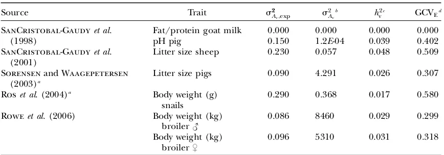
Av ¼0. As reviewed in the Introduction, there is empirical evidence that genotypes differ in environmental variance, but it is not abundant. To compare results of different studies ana-lyzing field data we use Equation 17, because some are based on the exponential genetic model (SanCristobal -Gaudyet al. 1998, 2001; Sorensenand Waagepetersen 2003; Roset al. 2004) and some on the additive genetic model (Roweet al. 2006). The measure of heritability (h2
v) developed in this study (Equation 13) and the genetic coefficient of variation for environmental variance GCVE¼sA=m¼sAv=s
2
E, denoted ‘‘evolvability’’ (Houle 1992), are used to compare results from different studies
(Table 9). Heritabilities of environmental variance were low, in the range 0.02–0.05 as used in this study, and GCVE’s were large, in the range of 0.30–0.58 (excluding 0). Note that GCV2Eis close tos2
Av;exp. The low values ofh 2 v show that a large amount of information is necessary to estimateAˆvaccurately, but the high values of GCVEshow that there is substantial opportunity for genetic change.
Other evidence of the existence of genetic hetero-geneity of environmental variance can come from selection experiments. With genetic heterogeneity of environmental variance, environmental variance would decrease with stabilizing selection and increase with disruptive selection. In most studies (e.g., Rendelet al. 1966; Cardin and Minvielle 1986), however, only changes in phenotypic variance are reported, which are not separated into changes in genetic and environ-mental variance. Interpretation of any selection exper-iment is complicated by possible changes in genetic variance due to gene frequency change, which cannot be predicted from simple base population parameters. Under infinitesimal model assumptions, effects of gene frequency change can be ignored and those due to gametic phase disequilibrium can be predicted. Due to negative gametic phase disequilibrium, genetic variance is expected to decrease with stabilizing selection and increase with disruptive selection (Bulmer 1971). In agreement with this expectation, Kaufmanet al. (1977) found substantial decreases in genetic and environmen-tal variance with stabilizing selection inT. castaneumand Scharlooet al. (1972) observed substantial increases in genetic and environmental variance with disruptive selec-tion inD. melanogaster, indicating a substantial genetic variance in environmental variance. Sorensenand Hill (1983), however, found large increases only in genetic variance with disruptive selection inD. melanogaster. TABLE 9
Comparison of literature estimates of genetic variance in environmental variance
Source Trait s2
Av;exp s
2 Av
b h2
v
c GCV
Ed
SanCristobal-Gaudyet al.
(1998)
Fat/protein goat milk 0.000 0.000 0.000 0.000
pH pig 0.150 1.2E-04 0.039 0.402
SanCristobal-Gaudyet al.
(2001)
Litter size sheep 0.230 0.057 0.048 0.509
Sorensenand Waagepetersen
(2003)a
Litter size pigs 0.090 4.291 0.026 0.307
Roset al. (2004)a Body weight (g)
snails
0.290 0.368 0.017 0.580
Roweet al. (2006) Body weight (kg)
broiler#
0.086 8460 0.029 0.299
Body weight (kg) broiler$
0.096 5310 0.031 0.318
a
Models included permanent environmental variance; environmental variance was taken from their model 1 estimates.
b
Equation 17:s2
Av¼s
4
E;expexpð2s 2
Av;expÞ s
4 E.
c h2
v ¼s 2 Av=ð2s
4 P13s
2
AvÞ ¼heritability of environmental variance.
d
GCVE¼sAv=s
2
Even though some studies analyzing field data or selection experiments show existence of genetic hetero-geneity of environmental variance, it could still be due to statistical artifacts,e.g., due to confounding genetic and environmental effects on variance or violation of the infinitesimal model assumption. If genetic hetero-geneity of environmental variance is a truly biological phenomenon, it could be due to scaling, genetic vari-ance in environmental sensitivity, or a combination of both. Traits seem to have a rather constant CV, even when the mean changes dramatically due to selection (Hilland Bu¨ nger2004). A constant CV would require a correlation of unity between mean and standard de-viation, which has not been found in analysis of field data (Sorensen and Waagepetersen 2003; Roset al. 2004; Roweet al. 2006). Genetic heterogeneity of environmental variance can arise from genetic differences in environ-mental sensitivity (Falconerand Mackay1996; Lynch and Walsh1998). When genotypes perform under var-iable environmental conditions, which are unknown to the researcher, genetic differences in response to environmental conditions may be observed as genetic heterogeneity of environmental variance.
Genetic heterogeneity of environmental variance is a complicated phenomenon and there is not yet abun-dant evidence of its existence. The results in this study may help in understanding the consequences of genetic heterogeneity of environmental variance on pheno-types and the methods can help in designing selection experiments and in evaluating breeding strategies or the effects of natural selection that change both the mean and the variance. Genetic heterogeneity of envi-ronmental variance may indeed be exploited to breed more ‘‘robust’’ or ‘‘stable’’ genotypes.
H.M. thanks Johan van Arendonk, Bart Ducro, and Roel Veerkamp for valuable comments on earlier versions of the manuscript. We thank Ian White for statistical advice. European Animal Disease Genomics Network of Excellence for Animal Health and Food Safety is acknowl-edged for financial support to a visit of H.M. to Edinburgh and the Biotechnology and Biological Sciences Research Council for research support to W.G.H.
LITERATURE CITED
Bulmer, M. G., 1971 The effect of selection on genetic variability. Am. Nat.105:201–211.
Cameron, N. D., 1997 Selection Indices and Prediction of Genetic Merit in Animal Breeding. CAB International, Wallingford, UK.
Cardin, S., and F. Minvielle, 1986 Selection on phenotypic varia-tion of pupa weight in Tribolium castaneum. Can. J. Genet. Cytol. 28:856–861.
Clay, J. S., W. E. Vinsonand J. M. White, 1979 Heterogeneity of daughter variances of sires for milk yield. J. Dairy Sci.62:985–989. Debat, V., and P. David, 2001 Mapping phenotypes: canalization, plas-ticity and developmental stability. Trends Ecol. Evol.16:555–561. Falconer, D. S., and T. F. C. Mackay, 1996 Introduction to
Quantita-tive Genetics. Pearson Education Limited, Essex, UK.
Falconer, D. S., and A. Robertson, 1956 Selection for environ-mental variability of body size in mice. Z. Indukt. Abstam-mungs-Vererbungsl.87:385–391.
Flatt, T., 2005 The evolutionary genetics of canalization. Q. Rev. Biol.80:287–316.
Foulley, F. L., and R. L. Quaas, 1995 Heterogeneous variances in Gaussian linear mixed models. Genet. Sel. Evol.27:211–228. Gavrilets, S., and A. Hastings, 1994 A quantitative-genetic model
for selection on developmental noise. Evolution48:1478–1486. Hazel, L. N., 1943 The genetic basis for constructing selection
in-dexes. Genetics28:476–490.
Henderson, C. R., 1984 Applications of Linear Models in Animal Breeding. University of Guelph, Guelph, Ontario, Canada.
Hill, W. G., 2004 Heterogeneity of genetic and environmental var-iance of quantitative traits. J. Ind. Soc. Agric. Stat.57:49–63. Hill, W. G., and L. Bu¨ nger, 2004 Inferences on the genetics of
quantitative traits from long-term selection in laboratory and do-mestic animals. Plant Breed. Rev.24(2): 169–210.
Hill, W. G., and X. S. Zhang, 2004 Effects of phenotypic variability of directional selection arising through genetic differences in re-sidual variability. Genet. Res.83:121–132.
Hill, W. G., and X. S. Zhang, 2005 Erratum Hill and Zhang (2004). Genet. Res.86:160.
Hohenboken, W. D., 1985 The manipulation of variation in quan-titative traits: a review of possible genetic strategies. J. Anim. Sci. 60:101–110.
Houle, D., 1992 Comparing evolvability and variability of quantita-tive traits. Genetics130:195–204.
Kaufman, P. K., F. D. Enfieldand R. E. Comstock, 1977 Stabilizing selection for pupa weight in Tribolium castaneum. Genetics87: 327–341.
Lynch, M., and B. Walsh, 1998 Genetics and Analysis of Quantitative Traits. Sinauer Associates, Sunderland, MA.
Mackay, T. F. C., and R. F. Lyman, 2005 Drosophila bristles and the nature of quantitative genetic variation. Philos. Trans. R. Soc. B. 360:1513–1527.
Rendel, J. M., B. L. Sheldonand D. E. Finlay, 1966 Selection for canalization of the scute phenotype. II. Am. Nat.100:13–31. Robertson, F. W., and E. C. R. Reeve, 1952 Heterozygosity,
environ-mental variation and heterosis. Nature170:286.
Ros, M., D. Sorensen, R. Waagepetersen, M. Dupont-Nivet, M. SanCristobalet al., 2004 Evidence for genetic control of adult weight plasticity in the snail helix aspersa. Genetics168: 2089–2097.
Rowe, S. J., I. M. S. White, S. Avendano and W. G. Hill, 2006 Genetic heterogeneity of residual variance in broiler chickens. Genet. Sel. Evol.38:617–635.
SanCristobal-Gaudy, M., J. M. Elsen, L. Bodin and C. Chevalet, 1998 Prediction of the response to a selection for canalisation of a continuous trait in animal breeding. Genet. Sel. Evol.30:423–451. SanCristobal-Gaudy, M., L. Bodin, J. M. Elsenand C. Chevalet, 2001 Genetic components of litter size variability in sheep. Genet. Sel. Evol.33:249–271.
Scharloo, W., 1991 Canalization: genetic and developmental as-pects. Annu. Rev. Ecol. Syst.22:65–93.
Scharloo, W., A. Zweep, K. A. Schuitemaand J. G. Wijnstra, 1972 Stabilizing and disruptive selection on a mutant character in Drosophila. IV. Selection on sensitivity to temperature. Genet-ics71:551–566.
Sorensen, D., and R. Waagepetersen, 2003 Normal linear models with genetically structured residual variance heterogeneity: a case study. Genet. Res.82:207–222.
Sorensen, D. A., and W. G. Hill, 1983 Effects of disruptive selec-tion on genetic variance. Theor. Appl. Genet.65:173–180. Stuart, A., and J. K. Ord, 1994 Kendall’s Advanced Theory of Statistics:
Distribution Theory. Arnold, London.
VanVleck, L. D., 1968 Variation of milk records within paternal-sib groups. J. Dairy Sci.51:1465–1470.
Waddington, C. H., 1942 Canalization of development and the in-heritance of acquired characters. Nature150:563–565. Waddington, C. H., 1960 Experiments on canalizing selection.
Genet. Res.1:140–150.
Wagner, G. P., G. Boothand H. Bagheri-Chaichian, 1997 A pop-ulation genetic theory of canalization. Evolution51:329–347. Zhang, X. S., and W. G. Hill, 2005 Evolution of the environmental
component of the phenotypic variance: stabilizing selection in changing environments and the cost of homogeneity. Evolution 59:1237–1244.
APPENDIX A: DERIVATION OF ELEMENTS IN THE P- AND G-MATRICES
Selection on a single phenotype:The elements in theP- andG-matrices were derived as follows, using the Roman E to denote expectation and the italic E to denote the environmental deviation E ¼x ffiffiffiffiffiffiffiffiffiffiffiffiffiffiffiffis2
E1Av p
and noting that Eðx2Þ ¼1:
EðPÞ ¼0;EðP2Þ ¼s2P;
EðP3Þ ¼EA3m13Am2E13AmE21E3¼01013EAms2E1Av10¼3covAmv;
EðP4Þ ¼E A4m14Am3E16A2mE214AmE31E4
¼3s4P13s2A
v;
EðP5Þ ¼E A5m15Am4E110Am3E2110A2mE315AmE41E5
¼30s2PcovAmv;
EðP6Þ ¼E A6m16Am5E115A4mE2120A3mE3115Am2E416AmE51E6
¼15s6P145s2Ps2A
ms
2
E190covA2mv145s
2 Ps2Av:
varðPÞ ¼EðP2Þ ðEðPÞÞ2; varðP2Þ ¼EðP4Þ fEðP2Þg2;
covðP;P2Þ ¼EðP3Þ EðPÞEðP2Þ;
covðP;P3Þ ¼EðP4Þ EðPÞEðP3Þ; covðP2;P3Þ ¼EðP5Þ EðP2ÞEðP3Þ;
varðP3Þ ¼EðP6Þ ðEðP3ÞÞ2:
covðP;AmÞ ¼s2A
m;
covðP2;AmÞ ¼cov Am2 12AmE1E2;Am
¼0101covðE2;AmÞ ¼covAmv;
covðP3;AmÞ ¼cov A3m13A2mE13AmE21E3;Am
¼cov A3m;Am
1cov 3AmE2;Am
¼3s4A
m13s
2
Ams
2
E¼3s2Ps2Am:
Similarly covðP;AvÞ ¼covAmv, cov P 2;A
v
ð Þ ¼s2
Av, and cov P 3;A
v
ð Þ ¼3s2 PcovAmv.
Selection based on a group of relatives:
varðPÞ ¼ s2
P1awðn1Þs2Am
!
=n
covðP;ðPÞ2Þ ¼ ncov Pk;P2
k
1nðn1ÞcovPk;Pl212 covðPk;PkPlÞ
=n3
¼hf313awðn1ÞgcovAmv
i
=n2
varððPÞ2Þ ¼
nvar Pk2 1nðn1Þ covPk2;Pl214 cov Pk2;PkPl
12 covðPkPl;PkPlÞ
1nðn1Þðn2Þ 2 cov Pk2;PlPm
14 covðPkPl;PkPmÞ
1nðn1Þðn2Þðn3ÞcovðPkPl;PmPnÞ
2 6 4
3 7 5
, n4
¼2 s2P1awðn1Þs2
Am
=n
h i2
1 f313awðn1Þgs2
Av
h i
=n3
varðP2Þ ¼nvarPk21nðn1ÞcovPk2;Pl2=n2¼ 2s4P13s2A
v
n o
1ðn1Þ 2aw2s4A
m1aws
2
Av
n o
h i.
n
covðP;P2Þ ¼
ncovPk;Pk21nðn1ÞcovPk;Pl2
=n2¼ ½f31awðn1ÞgcovAmv=n
covðP;varWÞ ¼ ½n=n13hcovðP;P2Þ covðP;ðPÞ2Þi¼ ½f31awðn3Þgcov