Simultaneous Detection of Linkage Disequilibrium and Genetic Differentiation of Subdivided Populations



DOI: 10.1534/genetics.103.023044

Simultaneous Detection of Linkage Disequilibrium and

Genetic Differentiation of Subdivided Populations

Shuichi Kitada*

,1

_{and Hirohisa Kishino}

†

*Faculty of Marine Science, Tokyo University of Marine Science and Technology, Minato, Tokyo 108-8477, Japan and †_{Graduate School of Agricultural and Life Sciences, University of Tokyo, Bunkyo, Tokyo 113-8657, Japan}

Manuscript received March 20, 2003 Accepted for publication December 26, 2003

ABSTRACT

We propose a new method for simultaneously detecting linkage disequilibrium and genetic structure in subdivided populations. Taking subpopulation structure into account with a hierarchical model, we estimate the magnitude of genetic differentiation and linkage disequilibrium in a metapopulation on the basis of geographical samples, rather than decompose a population into a finite number of random-mating subpopulations. We assume that Hardy-Weinberg equilibrium is satisfied in each locality, but do not as-sume independence between marker loci. Linkage states remain unknown. Genetic differentiation and linkage disequilibrium are expressed as hyperparameters describing the prior distribution of genotypes or haplotypes. We estimate related parameters by maximizing marginal-likelihood functions and detect linkage equilibrium or disequilibrium by the Akaike information criterion. Our empirical Bayesian model analyzes genotype and haplotype frequencies regardless of haploid or diploid data, so it can be applied to most commonly used genetic markers. The performance of our procedure is examined via numerical simulations in comparison with classical procedures. Finally, we analyze isozyme data of ayu, a severely exploited fish species, and single-nucleotide polymorphisms in humanALDH2.

W

ITH the many discoveries of fine-scale markers developed a method called the transmission/disequilib-rium test (TDT), which uses nuclear family data to de-that represent highly polymorphic loci, linkage

dis-tect real associations in structured populations. To use equilibrium between these markers and disease genes

this type of reliable information, similar family-based or other trait genes has regained importance (Jorde

methods for testing linkage disequilibrium have been 1995). Along with the rapid progress of genetic

tech-developed (e.g.,ExcoffierandSlatkin1998;

Lazze-niques, assessing linkage disequilibrium has become a

roni and Lange 1998; Spielman and Ewens 1998).

current concern. The assessment involves two aspects:

However, family-based methods cannot be used for asso-detecting the presence of disequilibrium and estimating

ciation studies of undomesticated species, such as wild-its magnitude once disequilibrium has been confirmed

life and forest trees, for which no nuclear family records (Weir 1979). Continuous efforts have been made on

are available (WuandZeng2001). Hence, population-such assessments of linkage disequilibrium between

al-based methods that detect linkage disequilibrium even leles at two or more loci (Hill1974a,b; Brown1975;

in the presence of population structure are required.

Weir andCockerham 1978;Slatkin and Excoffier

Pritchard et al. (2000a,b) proposed a

population-1996;Luo1998;LuoandSuhai1999;Luoet al.2000;

based method that can detect associations between

AyresandBalding2001;LuoandWu2001). Methods

marker alleles and phenotypes in structured popula-for linkage disequilibrium-based mapping of target

tions. The essential idea of the method is to decompose genes have also been developed (HillandWeir1994;

a sample drawn from a mixed population into several

Kaplanet al.1995;XiongandGuo1997;Meuwissen

unstructured subpopulations and test the association in

andGoddard2000;WuandZeng2001). These

meth-the homogeneous subpopulations. The methods have ods assume homogeneous natural populations.

How-been applied to association analyses in humans (Parra

ever, if a population is structured, this leads to biased

et al.1998;Rosenberget al.2002) and crop plants, with results (known as spurious association) that can reject

modified test statistics being used to deal with quantita-a null quantita-associquantita-ation between quantita-a phenotype quantita-and moleculquantita-ar

tive traits (Thornsberryet al.2001). markers (e.g.,LanderandSchork1994).

To study the population structure, a sample is often To overcome this problem, Spielman et al. (1993)

divided by geographical regions. However, in many cases, there are no obvious regional units by which subpopula-tions can be defined. Rather, natural populasubpopula-tions have

1_{Corresponding author:Tokyo University of Marine Science and}

Tech-a complex hierTech-archicTech-al structure, forming Tech-a metTech-apopu-

metapopu-nology, 4-5-7 Konan, Minato, Tokyo 108-8477, Japan.

E-mail: [email protected] lation (PannellandCharlesworth2000). In models,

a metapopulation has a continuous structure and con- lations that have reached equilibrium under the joint effects of drift and mutation or migration, Wright

sists of an infinite number of subpopulations, or demes.

Such populations are well described by hierarchical (1945, 1951) found that allele frequencies for loci with two alleles have a beta distribution; for multiallele loci, models that specify the distribution of genetic structure

among demes. Population subdivision (NeiandLi1973; the distribution is Dirichlet. We assumed that hyperpar-ameters are common over subpopulations and the sum

Petersonet al.1999) and other evolutionary forces such

as genetic drift (HillandRobertson1968), natural se- of the hyperparameters is also common for all loci. So, if random sampling of demes is performed from a lection (Lewontin1964), and mutation (Ohta1982a,b)

affect linkage disequilibrium. Therefore, when assess- metapopulation, estimated hyperparameters describe ing linkage disequilibrium in natural populations, it is the magnitude of genetic differentiation among sub-very important to also estimate the magnitude of genetic populations that have reached equilibrium. The mean

differentiation. linkage disequilibrium coefficient over subpopulations

In this article, we propose a new strategy to detect is also written as a function of the hyperparameters, as linkage disequilibrium between marker loci and simulta- shown later. Therefore, our assumption on hyperpara-neously estimate genetic differentiation in metapopula- meters has genetic meaning.

tions, extending the empirical Bayesian method of Now,Kdemes are randomly sampled from the

meta-Kitadaet al.(2000). Instead of decomposing a popula- population, and nk individuals are randomly sampled

tion into a finite number of subpopulations, we describe from each deme (k⫽ 1, . . . ,K). Given the allele fre-a distribution for fre-allele frequencies within subpopulfre-ations quencies at each deme, the sample counts of alleles, and test linkage disequilibrium using an information nk⫽ (nk1, . . . ,nkI)⬘, follow a multinomial distribution.

criterion based on hierarchical models that detect either Taking account of uncertainty of the allele frequen-linkage equilibrium or disequilibrium. Using samples cies, the likelihood of the sample counts is expressed from randomly sampled localities from a metapopulation, as a marginal-likelihood function, which is a Dirichlet-we estimate hyperparameters associated with linkage multinomial distribution (e.g., Lange 1995; Rannala

disequilibrium and genetic differentiation, on the basis and Hartigan 1996; Weir 1996; Kitada et al. 2000; of marginal-likelihood functions derived from prior dis- Balding2003):

tributions of allele or haplotype frequencies and

likeli-L˜(␣|nk)⫽

冮

. . .

冮

L(p|nk)␲(p|␣)dp

hood functions. We assume that individuals mate ran-domly and that Hardy-Weinberg (H-W) equilibrium holds

in each locality or deme. The method can be applied to _⫽ nk!

兿

nki!

⌫(␪)

⌫(␪ ⫹n)

兿

I

i⫽1

⌫(␣i⫹nki)

⌫(␣i)

. ₍₂₎

frequency data of common genetic markers, including

isozymes, mtDNA, microsatellites, and single-nucleotide _{The total likelihood is the product of the likelihoods} polymorphisms (SNPs). We do not assume independence

ofKdemes. Here,nk⫽

兺

Ii⫽1nki.

between marker loci, and linkage states remain unknown.

With a sample size ofn, the variance-covariance ma-We examine the performance of our procedure via

nu-trix of a Dirichlet-multinomial distribution is (n⫹ ␪)/ merical simulations in comparison with classical

proce-(1⫹ ␪) times larger than that of the multinomial distri-dures. Finally, we analyze isozyme data of ayu, a severely

bution (JohnsonandKotz1969). This phenomenon, exploited fish species, and single-nucleotide

polymor-in which the variance exceeds the nompolymor-inal variance, is phisms in humanALDH2.

called overdispersion. In our hierarchical models, over-dispersion corresponds to the variation of allele fre-quencies over subpopulations. With samples of size

MODELS AND METHODS

n1, . . ,nk, our overdispersion,␴2, becomes

Distribution of allele frequencies and genetic

differ-entiation:We consider a metapopulation that consists _␴2 _⫽n⫹ ␪

1⫹ ␪. (3)

of localities or demes. Hardy-Weinberg equilibrium holds in each deme. The distribution of the allele frequencies,

Here,nis the mean sample count overKsamples given p⫽(p1, . . . ,pI)⬘, at each deme is described as a

Dirich-byn⫽

兺

K

k⫽1nk/K. For a panmictic population,␴2 is 1;

let distribution (JohnsonandKotz1969),

it takes values⬎1 according to the magnitude of genetic differentiation among subpopulations. On the other

␲(p|␣)⫽ ⌫(␪)

兿

I

i⫽1⌫(␣i)

兿

I

i⫽1

p␣_ii⫺1, (1)

hand,␪converges to infinity for a panmictic population. From Weir’s equation (Weir 1996, p. 48, Equation whereIis the number of alleles and␪ ⫽

兺

I

i⫽1␣iand␣⫽ _{2.15), the variance of the allele frequency between}

sub-(␣1, . . . , ␣I)⬘ are regarded as hyperparameters for re- _{populations is expressed as}

spective alleles specifying prior distribution. We use this

distribution as a prior for allele frequencies of a subdi- _Var[p]⫽ p(1⫺p)

popu-TABLE 1

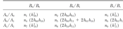
The termFST(2n⫺1)⫹1 corresponds to the dispersion parameter␴2_{. From this,Kitadaet al.(2000) obtained}

Notation for number of observed composite genotypes

the relation between␴2_andF

ST(Wright1951):

B0/B0 B0/B1 B1/B1

FST⫽ ␴ 2⫺₁

2n⫺ 1. (4) A0/A0 n1(h2

00) n2(2h00h01) n3(h201) A0/A1 n4(2h00h10) n5(2h00h11⫹2h01h10) n6(2h01h11)

If the organism is haploid, 2nshould ben. By substitut- A1/A1 n7(h2

10) n8(2h10h11) n9(h211) ing Equation 3 into Equation 4 and assumingn⫽2n, we

Diplotype probabilities are given in parentheses.

obtain the relation

FST⫽ 1

1⫹ ␪, (5) lations have a Dirichlet (for casesIj ⬎ 2) or beta (for

casesIj⫽2) distribution. The marginal-likelihood

func-which is also given inBalding(2003). From Equation _{tion for a subpopulation is obtained from Equations 1,}

5, we have _{2, and 7 as}

␪ ⫽ 1

FST

⫺1. (6) _L˜_{0(␣|n)⫽C⬘2}nhetero

兿

J

j⫽1

冦

⌫(␪)

⌫(␪ ⫹2n)

兿

I_j

i⫽1

⌫(␣(j)

i ⫹2n(ij))

⌫(␣(ij))

冧

, (8)

This coincides with Equation 3 ofRannalaand

Harti-where 2n(j)

i , the number of genes for allelei at locusj, gan(1996), which was proposed byWright(1969) and

is calculated from composite genotypes. The total likeli-gives the rate of gene flow. Thus, the sum of

hyperpara-hood is the product ofKlikelihood functions for respec-meters ␪ is consistent with the rate of gene flow and

samples. This equation can also be used for haploid has a relation withFST.

organisms by usingniandCinstead of 2niandC⬘2nhetero.

Linkage equilibrium with population structure:When

Linkage disequilibrium with population structure:

genetic data are available from multiple loci, the

likeli-The likelihood for sample haplotypes of a subpopula-hood is obtained as a product of the likelisubpopula-hoods of

tion is also a multinomial distribution: these loci when they are under linkage equilibrium. We

consider diploid organisms. Let the frequency allele i _L

1(p|n)⫽C

兿

i(1)...i(J)

(hi(1)...i(J))ni (1)_...i(J)

. (9)

in a subpopulation at locusjbep(j)

i (j⫽1, . . . ,J;i⫽

1, . . . ,Ij), whereJis the number of loci. The haplotype

If the haplotypes are observed, the marginal likelihood frequency of the subpopulation under linkage

equilib-is given by rium can be written by the product of allele frequencies

over the loci as

L˜1(␣|n)⫽C

⌫(␪)

⌫(␪ ⫹n)

兿

I

i⫽1

⌫(␣i⫹ni)

⌫(␣i)

, (10)

h_i(1) ...i(J)⫽p

(1)

i . . .p(iJ),

whereIis the number of haplotypes and, for simplicity, where the combination ofJallelesi(1)_{. . .i}(J)_{should be}

we use a suffix i for haplotypes instead of i(1) _{. . . i}(J)_.

i(1)

j . . .i(jJ), but we use ellipses for simplicity. Let the

sam-However, when analyzing diploid data, we do not ob-ple count for haplotypes be n_i(1)

...i(J) and 兺ni(1)...i(J)⫽2n

serve diplotypes (and then no haplotypes), but only (individuals). The likelihood for sample haplotypes

composite genotypes. under H-W equilibrium is a multinomial distribution,

When investigating linkage disequilibrium, the link-age phase between two alleles may be of most interest. L0(p|n)⫽C

兿

i(1)...i(J)

(p(1)

i · · ·p(iJ))ni

(1)

...i(J)⫽C

兿

J

j⫽1

兿

I_J

i⫽1 (p(j)

i )2n

(j) i ,

Hence, here we focus on models for two loci with two alleles and derive the general marginal-likelihood func-where 2n(j)

i is the number of genes of alleleiat locus

tion in theappendix. j. The constant termC ⫽2n!/⌸ini(1)...i(J)! is the

combina-Let allele frequencies for two loci be pA₀,pA₁andpB₀,

tion of the observed haplotypes. However, we do not

ob-pB₁, and let the haplotype frequencies beh00,h01,h10,h11in serve haplotypes but genotypes. When composite

geno-a subpopulgeno-ation. In this cgeno-ase, nine composite genotypes typesGi(1)...i(J)are observed, the likelihood is written as

can be observed with specific diplotypes. Let the number L0(p|n)⫽C⬘2nhetero

兿

i(1)_...i(J) (pG_i(1)

...i(J))

nG_i(1)_...i(J), (7) of individuals for the genotypes ben

1, . . . ,n9(Table 1). For example, the diplotype for the composite genotype A0A0B1B1can be specified byA0B1/A0B1. Under the H-W whereC⬘ ⫽n!/⌸i(1)...i(J)nG_i(1)

...i(J)! andnheterois the sum of the

equilibrium assumption, the probability of having the heterozygous loci overn individuals. Under H-W

equi-genotype ish2

01and that for A0B0/A0B1 is 2h00h01. Thus, librium, probabilities for heterozygous genotypes are

the probabilities of having genotypes can be written by obtained by duplicating the product of allele

frequen-diplotype probabilities, which are combinations of hap-cies. The term 2nhetero_{refers to such duplication.}

subpopu-two diplotypes are possible for the genotypes. In this

DˆTOTAL⫽ ␣

ˆ00␣ˆ11⫺ ␣ˆ01␣ˆ10

␪ˆ2 . (14)

case,A0A1B0B1is the double heterozygote with observed number n5. For this genotype, the possible diplotypes

However, this estimator is biased. LetE[D] be the mean are A0B0/A1B1 and A0B1/A1B0. The probability for the

ofDat each deme, which can be written as genotype is then given as 2h00h11⫹2h01h10(Table 1).

The likelihood of composite genotypes for the case _{E[D]⫽E[h00⫺pA}

0pB0]

of two loci with two alleles is given in Hudson (2001,

⫽E[h00]⫺E[pA0]E[pB0]⫹E[pA0]E[pB0]⫺E[pA0pB0]

p. 316, Equation 11.6). Expanding the term for the double

heterozygote, we obtain the likelihood function as _⫽

DTOTAL⫺Cov[pA0,pB0],

from which we have L1(p|n)⫽C⬘2n₂⫹n₄⫹n₅⫹n₆⫹n₈

兺

n5

t⫽0

冢

n5

t

冣

(h00)

2n₁⫹n₂⫹n₄⫹n₅⫺t_(h01)n₂⫹2n₃⫹n₆⫹t

DTOTAL⫽E[D]⫹ Cov[pA₀,pB₀]. (15) ⫻(h10)n4⫹2n7⫹n8⫹t_(h11)n5⫹n6⫹n8⫹2n9⫺t_, (11)

AspA₀⫽h00⫹ h01andpB₀ ⫽h00⫹h10, the covariance is whereC⬘ ⫽n!/⌸9

i⫽1ni! is a constant term for the combina- expressed as

tion of the multinomial likelihood. The

marginal-likeli-Cov[pA₀,pB₀]⫽Var[h00]⫹Cov[h00,h10]⫹Cov[h00,h01] hood function for a subpopulation is then obtained as

⫹ Cov[h01,h10]. L˜1(␣|n)⫽C⬘2n2⫹n4⫹n5⫹n6⫹n8兺

n5

t⫽0

冢

n5

t

冣

⌫(␪)

⌫(␪ ⫹2n)

The variance and covariance of a Dirichlet distribution are Var[pi]⫽ ␣i(␪i⫺ ␣i)/(␪2(␪ ⫹1)) and Cov[pi,pj]⫽ ⫻ ⌫(␣00⫹2n1⫹n2⫹n4⫹n5⫺t)

⌫(␣00)

⌫(␣01⫹n2⫹2n3⫹n6⫹t)

⌫(␣01) ␣i␣j/(␪2(␪ ⫹1)) (JohnsonandKotz1969). Hence, we

have the covariance as a function of hyperparameters: ⫻ ⌫(␣10⫹n4⫹2n7⫹n8⫹t)

⌫(␣10)

⌫(␣11⫹n5⫹n6⫹n8⫹2n9⫺t)

⌫(␣11)

,

Cov典 [pA₀,pB₀]⫽ ␣

ˆ00␣ˆ11⫺ ␣ˆ01␣ˆ10

␪

ˆ2₍␪_ˆ ⫹ ₁₎ . (16) (12)

where␣11⫽ ␪ ⫺ ␣00⫺ ␣01⫺ ␣10. From Equations 14, 15, and 16, we have the unbiased

Parameter estimation and model selection: We esti- _{estimator of the mean linkage disequilibrium coefficient}

mate parameters by maximizing the negative log mar- _{correcting spurious association as} ginal-likelihood functions for linkage equilibrium and

disequilibrium. The constant terms C and C⬘ can be _Eˆ[D]⫽ ␣ˆ00␣ˆ11⫺ ␣ˆ01␣ˆ10

␪

ˆ(␪ˆ _{⫹ 1)} , (17)

excluded from the estimation procedure. We

reparame-terize hyperparameters with FST by using the relation _{while correction ofris not trivial because of the} denomi-given by Equation 6 and estimateFSTand hyperparamet- _{nator of Equation 13.}

ers numerically as free parameters by using simplex _{We use the Akaike Information Criterion (AIC;Akaike} minimization. The rate of gene flow␪and the dispersion _{1973) as a criterion for model selections,}

parameter␴2_{are then estimated by Equations 4 and 6.}

AIC⫽2⫻LL典 ⫹2⫻ u, (18) Our empirical Bayesian procedure thus offers

maxi-mum-likelihood estimators of genetic differentiation. _{where LL}典 _{is the maximum marginal log-likelihood of} We estimate the 95% confidence interval for FSTfrom _{the model anduis the number of free parameters} esti-the log-likelihood profile, and esti-then estimate 95% con- _{mated. We can compare various models by this criterion;} fidence intervals for␪and␴2_{by substituting the lower}

the model with the lowest AIC value is selected as the and upper confidence limits ofFSTinto Equations 4 and most parsimonious model. Equation 18 indicates that,

6, respectively. _{when there are several models with similar values of the}

We also estimate the linkage correlation coefficient _{maximum likelihood, we should select the model with}

(HillandRobertson 1968) as _{the smallest number of parameters, again following the}

principle of parsimony. By using AIC, we can detect link-age equilibrium or disequilibrium.

rˆ⫽ DˆTOTAL

冪

Eˆ[pA₀](1⫺ Eˆ[pA₀])Eˆ[pB₀](1⫺Eˆ[pB₀])

, ₍₁₃₎

TESTING PERFORMANCE

whereE[pA0] andE[pB0] are mean allele frequencies over To evaluate the performance of our method, we con-ducted two sets of simulations. The first simulation ex-subpopulations, which are estimated from sample allele

rium with two other commonly used estimates: an esti- erated from the Dirichlet distribution, where the hyper-parameters were given as␣00⫽ ␪(0.64⫹0.16r), ␣01⫽ mate from a pooled sample and an average of the

esti-␣10 ⫽ ␪0.16(1 ⫺ r), and ␣11 ⫽ ␪(0.04 ⫹ 0.16r). We mated linkage disequilibrium over subsamples.

set total sample size to 1000 individuals and generated

Simulated data 1:We assumed that the mean

popula-haplotype frequencies for different numbers of locali-tion allele frequencies of the two loci over

subpopula-ties (K⫽ 10, 20, 40, 100) under various r(0, 0.2, 0.4, tions wereE[pA0]⫽E[pB0]⫽0.5 and hence haplotype

0.6, 0.8) with fixedFST⫽0.2. We then calculated sample frequencies were E[h00] ⫽ E[h11] ⫽ 0.25(1 ⫹ r) and

composite genotype counts on the basis of haplotype E[h01]⫽E[h10]⫽0.25(1⫺r). We set the sample size to

frequencies assuming H-W equilibrium. 50 individuals for each sampling point and generated

We estimatedFST,E[D], and hyperparameters on the haplotype frequencies for 20 geographical samples

un-basis of Equations 8, 12, and 17 for 1000 replicates. der variousFST(0, 0.05, 0.10, 0.15, 0.20) andr(0, 0.2,

DMEAN and DPOOL were estimated by the method of Hill 0.4, 0.6, 0.8). We then calculated sample composite

(1974b) on the basis of sample composite genotype genotype counts on the basis of haplotype frequencies

counts at each locality and the pooled counts. A larger assuming H-W equilibrium.

number of sampling points improved the precision of For the state of linkage equilibrium (r ⫽ 0), given

estimates ofFST(Table 3). Our hierarchical model esti-theFSTvalues, sample allele frequencies of two loci were

mated the real values ofE[D] correctly over the whole generated independently from the beta distribution

range of linkage disequilibrium and numbers of

sam-␤(␪/2,␪/2), where␪ ⫽1/FST⫺1. Haplotype

frequen-pling points. Precision of the estimates ofE[D] was also cies were then calculated asE[pA₀]E[pB₀] forE[h00]. Other

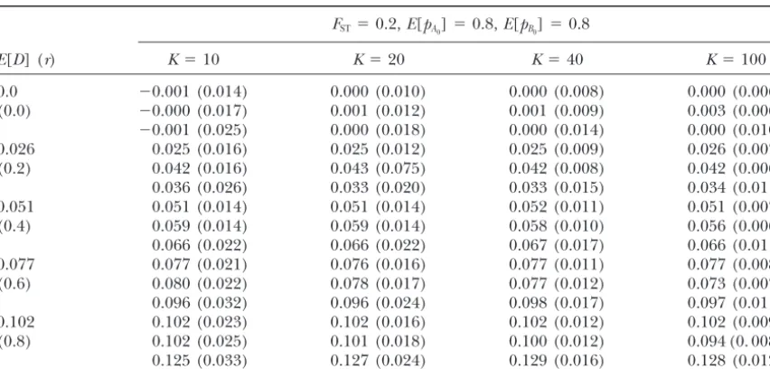
improved for a larger number of sampling points (Table haplotypes were calculated in a similar way. For the case

4). Estimates ofDMEAN were biased for weaker linkage ofFST⫽0, sample allele frequencies of the two loci were

disequilibrium. The biases were decreased for largerr; generated independently from the binomial

distribu-however, the biases were larger than those from the tion Bi(50, 0.5). For linkage disequilibrium, given the

hierarchical model. Estimates ofDPOOLwere largely

bi-FSTvalues, haplotype frequencies were generated from

ased with low precision over the whole range of linkage the Dirichlet distributionD(␣00,␣01,␣10,␣11), where the

disequilibrium and numbers of sampling points. The hyperparameters were given as␣00⫽ ␣11⫽ 0.25␪(1 ⫹

results showed that our method works more efficiently r) and␣01⫽ ␣10⫽ 0.25␪(1⫺ r). For cases ofFST⫽0,

than classical procedures. sample haplotype frequencies were generated from the

multinomial distribution Mul(50,E[h00], E[h01],E[h10],

E[h11]). APPLICATION TO REAL DATA

We estimatedFST,r, and hyperparameters on the basis _{Genotype data of the ayu:We analyzed isozyme} geno-of Equations 8, 12, and 13 for 1000 replicates. For all

type data for seven samples of the ayu (Plecoglossus alti-cases with r⬎ 0, the model of linkage disequilibrium

velis) from Japan (K. Yoshizawa, unpublished data). had smaller values of AIC and was selected. On the

Two samples of wild stocks were taken from Biwako Lake other hand, for all cases ofr⫽0, the model of linkage

(land-locked type) and Nagara River (amphidoromous equilibrium was selected. Estimates obtained from the

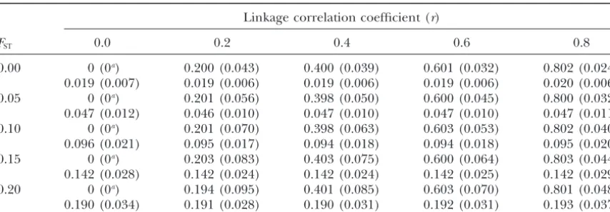
type), and five samples were taken from captive brood best-fit model agreed well with the real values ofFSTand _{stocks in hatcheries. The lifespan of ayu is 1 year. These}

r, showing that our method works appropriately over a _{brood stocks have been bred in captivity for between 7} wide range of genetic differentiation and linkage dis- _{and 26 generations in each hatchery to produce} juve-equilibrium (Table 2). _{niles for release to enhance severely exploited stocks.}

Simulated data 2: In an ordinary way, researchers _{The numbers of generations of captive breeding are}

would use the sample mean of the linkage disequilib- _{shown in parentheses with the names of the sampling} rium coefficient in each subpopulation (say,DMEAN) as _{locations in the Table 5 legend. Two loci were analyzed.} an estimator of the mean linkage disequilibrium coeffi- _{Four alleles were found at theGpilocus and three alleles} cient. Although a larger number of sampling points _{at theMpilocus. However, two alleles ofGpiand one of} should improve precision of estimates of genetic differ- _{Mpiwere very minor, and so we grouped them with major} entiation, limited sample size in each locality may result _{ones to obtain nine composite genotypes (Table 5).} in a poor estimate ofDMEAN. Another procedure is to esti- We estimated parameters on the basis of composite mate the mean linkage disequilibrium coefficient from _{genotype data by using Equations 8, 12, and 13 (Table 6).} pooled genotype data over subpopulations (say,DPOOL). A smaller AIC value was obtained for the model of link-This procedure neglects the population structure. age equilibrium; thus, linkage equilibrium betweenGpi The mean population allele frequencies of the two loci andMpiloci was detected. Estimates ofFSTand␪showed over subpopulations were assumed asE[pA₀]⫽E[pB₀]⫽0.8 very large genetic differentiation and small gene flow.

Generally, genetic differentiation of fish species is small and hence haplotype frequencies were E[h00]⫽ 0.64 ⫹

0.16r,E[h01]⫽E[h10]⫽0.16(1⫺r), andE[h11]⫽0.04⫹ because of large gene flows caused by migration or lack of barriers (e.g.,McPhersonet al.2001;Goldand

gen-TABLE 2

Mean linkage correlation coefficientsrandFSTof the best-fit models estimated from 1000 simulations

under various levels of linkage disequilibrium and population structure

Linkage correlation coefficient (r)

FST 0.0 0.2 0.4 0.6 0.8

0.00 0 (0a_{) 0.200 (0.043) 0.400 (0.039) 0.601 (0.032) 0.802 (0.024)}

0.019 (0.007) 0.019 (0.006) 0.019 (0.006) 0.019 (0.006) 0.020 (0.006)

0.05 0 (0a_{) 0.201 (0.056) 0.398 (0.050) 0.600 (0.045) 0.800 (0.032)}

0.047 (0.012) 0.046 (0.010) 0.047 (0.010) 0.047 (0.010) 0.047 (0.011)

0.10 0 (0a_{) 0.201 (0.070) 0.398 (0.063) 0.603 (0.053) 0.802 (0.040)}

0.096 (0.021) 0.095 (0.017) 0.094 (0.018) 0.094 (0.018) 0.095 (0.020)

0.15 0 (0a_{) 0.203 (0.083) 0.403 (0.075) 0.600 (0.064) 0.803 (0.044)}

0.142 (0.028) 0.142 (0.024) 0.142 (0.024) 0.142 (0.025) 0.142 (0.029)

0.20 0 (0a_{) 0.194 (0.095) 0.401 (0.085) 0.603 (0.070) 0.801 (0.048)}

0.190 (0.034) 0.191 (0.028) 0.190 (0.031) 0.192 (0.031) 0.193 (0.037)

The sample size was set to 50 individuals for each sampling point and haplotype frequencies for 20 geographi-cal samples were generated. The mean allele frequencies of the two loci were assumed asE[pA0]⫽E[pB0]⫽0.5. The numbers in parentheses are the standard errors of the estimates.

a_{In all replicates, the model of linkage equilibrium was selected.}

ner2002). However, the result obtained here is natural to 0.01 for 17 subpopulations, with an average of⫺0.45

(Petersonet al.1999, Table 4). Strong linkage

disequi-because the sample comprised three different groups:

land-locked, amphidoromous, and captive brood stocks librium was found, which is consistent with the analyses by Petersonet al. Estimates ofFSTand␪also showed that in successive breeding for many generations.

Human SNPs:We analyzed SNPs reported byPeter- genetic differentiation of humanALDH2was large with

a small gene flow.

sonet al.(1999) in the human aldehyde dehydrogenase 2 geneALDH2.

We focused on sites 1 and 2 from the six sites reported

DISCUSSION

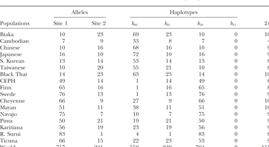
by Petersonet al.The haplotype frequencies were

esti-mated from the haplotype configurations given in their We have proposed a new method, based on genotype frequencies of geographical samples, to detect linkage Table 2 ash11⫽ H1 ⫹ H4 ⫹ H6 ⫹ H8 ⫹ H9, h12⫽ H3,

h21⫽H2, and h22⫽ 0. We estimated parameters using disequilibrium between markers and to simultaneously estimate genetic differentiation by taking population Equation 8 from the allele frequencies at the two sites

withinALDH2genotyped in 756 people from 17 popula- subdivision into account. The method detected linkage disequilibrium and estimated linkage disequilibrium co-tions across five continents (Table 7). We also estimated

parameters for estimated haplotypes on the basis of efficient andFSTcorrectly.

With a hierarchical model, we estimate the genetic Equation 10 (Tables 7 and 8). The AIC value for the

model of linkage disequilibrium was smaller than that structure in a metapopulation, rather than decompose a population into a finite number of randomly mating for linkage equilibrium. Our estimate of r was ⫺0.60,

whereas the original authors’ estimates varied from⫺0.96 subpopulations. The sum of hyperparameters␪coincided

TABLE 3

MeanFSTestimated from 1000 simulations under various levels of linkage disequilibrium

for different numbers of sampling points

FST⫽0.2,E[pA0]⫽0.8,E[pB0]⫽0.8

r K⫽10 K⫽20 K⫽40 K⫽100

0 0.180 (0.047) 0.193 (0.036) 0.195 (0.027) 0.198 (0.020)

0.2 0.181 (0.048) 0.193 (0.037) 0.196 (0.028) 0.198 (0.021)

0.4 0.180 (0.049) 0.190 (0.036) 0.195 (0.028) 0.198 (0.022)

0.6 0.183 (0.052) 0.192 (0.039) 0.197 (0.030) 0.198 (0.023)

0.8 0.183 (0.056) 0.191 (0.044) 0.197 (0.034) 0.198 (0.025)

TABLE 4

Performance of the hierarchical model in comparison with classical procedures

FST⫽0.2,E[pA0]⫽0.8,E[pB0]⫽0.8

E[D] (r) K⫽10 K⫽20 K⫽40 K⫽100

0.0 ⫺0.001 (0.014) 0.000 (0.010) 0.000 (0.008) 0.000 (0.006)

(0.0) ⫺0.000 (0.017) 0.001 (0.012) 0.001 (0.009) 0.003 (0.006)

⫺0.001 (0.025) 0.000 (0.018) 0.000 (0.014) 0.000 (0.010)

0.026 0.025 (0.016) 0.025 (0.012) 0.025 (0.009) 0.026 (0.007)

(0.2) 0.042 (0.016) 0.043 (0.075) 0.042 (0.008) 0.042 (0.006)

0.036 (0.026) 0.033 (0.020) 0.033 (0.015) 0.034 (0.011)

0.051 0.051 (0.014) 0.051 (0.014) 0.052 (0.011) 0.051 (0.007)

(0.4) 0.059 (0.014) 0.059 (0.014) 0.058 (0.010) 0.056 (0.006)

0.066 (0.022) 0.066 (0.022) 0.067 (0.017) 0.066 (0.011)

0.077 0.077 (0.021) 0.076 (0.016) 0.077 (0.011) 0.077 (0.008)

(0.6) 0.080 (0.022) 0.078 (0.017) 0.077 (0.012) 0.073 (0.007)

0.096 (0.032) 0.096 (0.024) 0.098 (0.017) 0.097 (0.011)

0.102 0.102 (0.023) 0.102 (0.016) 0.102 (0.012) 0.102 (0.009)

(0.8) 0.102 (0.025) 0.101 (0.018) 0.100 (0.012) 0.094 (0. 008)

0.125 (0.033) 0.127 (0.024) 0.129 (0.016) 0.128 (0.012)

Total sample size was fixed at 1000 individuals. The numbers are means estimated from 1000 simulations with standard errors in parentheses. Lines are arranged in threes as follows: top (E[D]), mean of the linkage correlation coefficient at each deme estimated by the hierarchical model; middle (DMEAN), sample mean of the linkage disequilibrium coefficient in each deme; bottom (DPOOL), estimates of the linkage disequilibrium coefficient based on pooled genotypes over demes.

with the rate of gene flow, andFSTwas written by␪. We territory. Even for marine fish, which can disperse widely because of the lack of barriers in oceans, the stock con-also showed by Equation 17 that the magnitude of

link-age disequilibrium depends on that of genetic differen- cept is popular in fishery resource management (Waples

1998). In breeding seasons, fish species generally gather tiation. Our model assumes metapopulations, which

in-cludes Wright’s island model as a special case (Wright to spawning grounds where they mate randomly. As a result of such breeding patterns, the assumption of 1940); hence the relationship between␪andFSTcan be

applied for these population models. The metapopula- Hardy-Weinberg equilibrium may be valid in each local-ity. Furthermore, in humans, whose population struc-tion concept fits with ecology of wildlife that have

lim-ited movement ability and may mate randomly in their tures may be more complex than those of wildlife, it has

TABLE 5

Allozyme composite genotype frequencies for seven samples of the ayu from Japan

Sampling location

Genotypes GM-1a _GM-2a _NGa _GFb _SGc _HSa _OTa

A0A0B0B0 1 1 65 32 4 3 79

A0A0B0B1 0 2 25 8 7 2 0

A0A0B1B1 0 0 1 2 3 0 0

A0A1B0B0 9 9 7 41 14 30 30

A0A1B0B1 17 18 2 5 27 23 0

A0A1B1B1 9 7 0 2 16 5 0

A1A1B0B0 18 17 0 7 5 19 2

A1A1B0B1 35 36 0 3 18 16 0

A1A1B1B1 11 10 0 1 6 2 0

Total 100 100 100 100 100 100 111

GM, Gunma (26); NG, Niigata (7); GF, Gifu; SG, Shiga; HS, Hiroshima (21); and OT, Oita (11) Prefecture. Numbers in parentheses are the numbers of generations in captive breeding.

a_{Captive brood stocks.}

b_{Wild (amphidoromous type).}

TABLE 8 TABLE 6

Estimated linkage correlation coefficient between Estimated worldwide linkage correlation coefficient between

sites 1 and 2 in the humanALDH2gene and genetic

GpiandMpiloci and genetic differentiation

among seven samples of ayu differentiation among 17 human populations

Models Models

Linkage Linkage

Linkage Linkage

equilibrium disequilibrium equilibrium disequilibrium

LLa ⫺_1444.79 ⫺_1247.85

LLa ⫺_1073.25 ⫺_1093.89

AIC 2152.50 2195.78 AIC 2895.58 2503.70

r — ⫺0.601

r — 0.024

FST 0.280 [0.168, 0.455] 0.209 FST 0.204 0.234 [0.166, 0.295]

␪ 3.908 3.267 [2.390, 5.024]

␪b _{2.576 [1.198, 4.952] 3.787}

␴2c _{29.164 [17.920, 46.825] 22.039 ␴}2 _{18.917 21.608 [15.598, 26.943]}

a_{Maximum log-likelihood without the multinomial} con-a_{Maximum log likelihood without the multinomial constant}

termC⬘in Equations 8 and 12. stant termCin Equations 8 and 10.

b_{Rate of gene flow.}

c_{Dispersion parameter.}

this treatment was appropriate. Consider a simple case of three haplotypes with sample countsn1,n2, and n3, been reported that geographic clusters often correspond _{where n}

3 ⫽ 0. The marginal-likelihood function for a closely to predefined regional or population groups or _{subpopulation is a Dirichlet-multinomial distribution:} collections of geographically similar populations (

Rosen-L1(␣1,␣2,␣3|n1,n2,n3)⫽ ⌫

(␣1⫹ ␣2⫹ ␣3)

⌫(␣1⫹ ␣2⫹ ␣3⫹n1⫹n2)

⌫(␣1⫹n1)

⌫(␣1)

⌫(␣2⫹n2)

⌫(␣2)

.

berget al.2002). In actual populations, various levels of

subdivision may exist (Excoffier2001), and the num- ₍₁₉₎

ber of demes should be very large with continuous

sub-Using the relation of⌫(n⫹1)⫽n⌫(n), the first term division. In ecological studies, sampling points may

in-of this equation can be written as crease year by year, which increases the accuracy of our

method. ⌫(␣1⫹ ␣2⫹ ␣3)

⌫(␣1⫹ ␣2⫹ ␣3)(␣1⫹ ␣2⫹ ␣3⫹1) . . . (␣1⫹ ␣2⫹ ␣3⫹n1⫹n2⫺1)

Estimates of hyperparameters were based only on

fre-quencies counted in the samples, and alleles that did not ⫽{(␣1⫹ ␣2⫹ ␣3⫹1) . . . (␣1⫹ ␣2⫹ ␣3⫹n1⫹n2⫺1)}⫺1.

(20) appear were assigned frequency 0. Here, we consider if

TABLE 7

Haplotype frequencies at two sites (sites 1 and 2) in the humanALDH2gene among 17 human populations,

calculated from Table 2 ofPetersonet al.(1999)

Alleles Haplotypes

Populations Site 1 Site 2 h00 h01 h10 h11 2n

Biaka 10 23 69 23 10 0 102

Cambodian 7 9 33 8 7 0 48

Chinese 10 16 68 16 10 0 94

Japanese 16 10 72 10 16 0 98

S. Korean 13 14 53 14 13 0 80

Taiwanese 10 20 55 21 10 0 86

Black Thai 14 23 63 23 14 0 100

CEPH 49 14 1 14 49 0 64

Finn 65 16 1 16 65 0 82

Swede 76 13 1 13 76 0 90

Cheyenne 66 9 27 9 66 0 102

Mayan 51 11 38 11 51 0 100

Navajo 75 7 10 7 75 0 92

Pima 50 21 19 21 50 0 90

Karitiana 56 19 23 19 56 0 98

R. Surui 83 1 4 1 83 0 88

Ticuna 66 15 22 23 53 0 98

Hudson, R. R., 2001 Linkage disequilibrium and recombination,

Hence, to maximize Equation 19, the term in the

paren-pp. 309–324 in Handbook of Statistical Genetics, edited by D. J.

theses in Equation 20 should be minimized. As␣3ⱖ0, _{Balding, M.Bishopand C.Cannings. Wiley, Chichester, UK.}

Johnson, N. L., and S.Kotz, 1969 Discrete Distributions. Wiley, New

the maximum-likelihood estimate of␣3 is then 0. This

York.

can be generalized for all cases.

Jorde, L. B., 1995 Linkage disequilibrium as a gene mapping tool.

For diploid data, we have two procedures for inferring _{Am. J. Hum. Genet.56:11–14.}

Kaplan, N., W. G. HillandB. S. Weir, 1995 Likelihood methods

linkage disequilibrium. The first procedure (method 1)

for locating disease genes in nonequilibrium populations. Am.

estimates hyperparameters using Equation 12 or the last

J. Hum. Genet.56:18–32.

equation in the appendix, on the basis of observed _{Kitada, S., T. HayashiandH. Kishino, 2000 Empirical Bayes}

proce-dure for estimating genetic distance between populations and

composite genotypes. Another way (method 2) is to

effective population size. Genetics156:2063–2079.

use Equation 10, on the basis of estimated haplotypes.

Lander, E. S., andN. J. Schork, 1994 Genetic dissection of complex

Several methods for estimating haplotype frequencies _{traits. Science265:2037–2048.}

Lange, K., 1995 Application of the Dirichlet distribution to forensic

have been developed (Excoffier and Slatkin 1995;

match probabilities. Genetica96:107–117.

Longet al.1995;SlatkinandExcoffier1996). In the

Lazzeroni, L. C., and K. Lange, 1998 A conditional inference

analysis of human SNPs, we used estimated haplotypes _{framework for extending the transmission/disequilibrium test.}

Hum. Hered.48:67–81.

as if they were observed data. However, the effect of

us-Lewontin, R. C., 1964 The interaction of selection and linkage. I.

ing estimated haplotypes on parameter estimates is

un-General considerations; heterotic models. Genetics49:4–67.

known. The accuracy of the inference might depend on _{Long, J. C., R. C.Williamsand M.Urbanek, 1995 An E-M algorithm}

and testing strategy for multiple-locus haplotypes. Am. J. Hum.

the precision of haplotype estimates. Method 1 should

Genet.56:799–810.

be better for accurate inference, but deriving explicit

Luo, Z. W., 1998 Detecting linkage disequilibrium between a

poly-marginal-likelihood functions becomes much harder _{morphic marker locus and a trait locus in natural populations.}

Heredity80:198–208.

for larger numbers of loci, although the general form

Luo, Z. W., andS. Suhai, 1999 Estimating linkage disequilibrium

of the marginal-likelihood function is derived in the

between a polymorphic marker locus and a trait locus in natural

appendix. Method 2 is much easier and more practical. _{populations. Genetics151:359–371.}

Luo, Z. W., andC.-I Wu, 2001 Modeling linkage disequilibrium

Precise estimation of haplotype frequencies is very

im-between a polymorphic marker locus and a locus affecting

com-portant for studies of linkage disequilibrium.

plex dichotomous traits in natural populations. Genetics 158:

1785–1800. We thank Kazutomo Yoshizawa for allowing us to use his

unpub-Luo, Z. W., S. H. TaoandZ-B. Zeng, 2000 Inferring linkage

disequi-lished data and Laurent Excoffier and an anonymous reviewer for their

librium between a polymorphic marker locus and a trait locus constructive comments on earlier versions of the manuscript. This

in natural populations. Genetics156:457–467.

work was supported by the Japan Society for the Promotion of Science

McPherson, A. A., R. L. Stephenson, P. T. O’Reilly, M. W. Jones

and Japan Science and Technology Agency.

andC. T. Taggart, 2001 Genetic diversity of coastal Northwest

Atlantic herring population implications for management. J. Fish

Biol.59:356–370.

Meuwissen, T. H. E., andM. E. Goddard, 2000 Fine mapping of

LITERATURE CITED

quantitative trait loci using linkage disequilibria with closely

linked marker loci. Genetics155:421–430.

Akaike, H., 1973 Information theory and an extension of the

maxi-mum likelihood principle, pp. 267–281 inThe Second International Nei, M., and W.-H. Li, 1973 Linkage disequilibrium in subdivided

populations. Genetics75:213–219.

Symposium on Information Theory, edited by B. N.Petrovand F.

Csa´ki. Akade´miai Kiado´, Budapest. Ohta, T., 1982a Linkage disequilibrium due to random genetic

drift in finite subdivided populations. Proc. Natl. Acad. Sci. USA

Ayres, K. L., andD. J. Balding, 2001 Measuring gametic

disequilib-rium from multilocus data. Genetics157:413–423. 79:1940–1944.

Ohta, T., 1982b Linkage disequilibrium with the island model.

Ge-Balding, D. J., 2003 Likelihood-based inference for genetic

correla-tion coefficient. Theor. Popul. Biol.63:221–230. netics75:139–155.

Pannell, J. R., andB. Charlesworth, 2000 Effects of

metapopula-Brown, A. D. H., 1975 Sample sizes required to detect linkage

dis-equilibrium between two or three loci. Theor. Popul. Biol.8:184–201. tion processes on measures of genetic diversity. Philos. Trans. R.

Soc. Lond. B355:1851–1864.

Excoffier, L., 2001 Analysis of population subdivision, pp. 271–307

inHandbook of Statistical Genetics, edited by D. J. Balding, M. Parra, E. J., A. Marcini, J. Akey, J. Maartinson, M. A. Batzeret al.,

1998 Estimating African American admixture proportions by

Bishopand C.Cannings. Wiley, Chichester, UK.

Excoffier, L., andM. Slatkin, 1995 Maximum likelihood estima- use of population-specific alleles. Am. J. Hum. Genet.63:1839–

1851. tion of molecular haplotype frequencies in a diploid population.

Mol. Biol. Evol.12:921–927. Peterson, R. J., D. GoldmanandJ. C. Long, 1999 Effects of

world-wide population subdivision onALDH2linkage disequilibrium.

Excoffier, L., andM. Slatkin, 1998 Incorporating genotypes of

relatives into a test of linkage disequilibrium. Am. J. Hum. Genet. Genet. Res.9:844–852.

Pritchard, J. K., M. Stephens, N. A. RosenbergandP. Donnelly,

62:171–180.

Gold, J. R., andT. F. Turner, 2002 Population structure of red drum 2000a Association mapping in structured populations. Am. J.

Hum. Genet.67:170–181.

(Sciaenops ocellatus) in the northern Gulf of Mexico, as inferred

from variation in nuclear-encoded microsatellites. Marine Biol.140: Pritchard, J. K., M. StephensandP. Donnelly, 2000b Inference

of population structure using multilocus genotype data. Genetics 249–265.

Hill, W. G., 1974a Tests for association of gene frequencies at sev- 156:945–959.

Rannala, B., andJ. A. Hartigan, 1996 Estimating gene flow in

eral loci in random diploid populations. Biometrics31:881–888.

Hill, W. G., 1974b Estimation of linkage disequilibrium in randomly island populations. Genet. Res.67:147–158.

Rosenberg, N. A., J. K. Pritchard, J. L. Weber, H. M. Cann, K. K.

mating populations. Heredity33:229–239.

Hill, W. G., andA. Robertson, 1968 Linkage disequilibrium in Kiddet al., 2002 Genetic structure of human populations.

Sci-ence298:2381–2384.

finite populations. Theor. Appl. Genet.38:226–231.

Hill, W. G., andB. S. Weir, 1994 Maximum likelihood estimation Slatkin, M., andL. Excoffier, 1996 Testing for linkage

disequilib-rium in genotype data using the EM algorithm. Heredity76:377–383.

of gene location by linkage disequilibrium. Am. J. Hum. Genet.

in the presence of association: the sib

transmission/disequilib-rium test. Am. J. Hum. Genet.62:450–458. L1⫽ C⬘

兿

m

i⫽1

冢

兺

l_Gi

j⫽1

PD_j

冣

n_Gi

.

Spielman, R. S., R E. McGinnisandW. J. Ewens, 1993 Transmission

test for linkage disequilibrium: the insulin gene region and

insu-lin-dependent diabetes mellitus (IDDM). Am. J. Hum. Genet.52: By multinomial expansion, we have another form of the

506–513. _{likelihood as}

Thornsberry, J. M., M. M. Goldman, J. Doebley, S. Kresovich,

D. Nielsenet al., 2001 Dwarf8 polymorphisms associate with

variation in flowering time. Nat. Genet.28:286–289.

L1⫽ C⬘

兺

i1...ilG₁

nG₁!

i(1)1 ! . . .i(1)l_G 1!

冢

Pi

(1) 1

D(G1)

1 . . .P

i_l(1)

G1 D(G1)

lG₁

冣

. . .

Waples, R. S., 1998 Separating the wheat from the chaff. Pattern

of genetic differentiation in high gene flow species. J. Hered.89:

438–450.

Weir, B. S., 1979 Inferences about linkage disequilibrium.

Biomet-兺

i₁...i_l

Gm

nGm!

i(1m)! . . .i (m)

l_Gm!

冢

Pi

(m) 1

D(Gm) 1 . . .P

i(lGm_m)

D(Gm) lGm

冣

,

rics35:235–254.

Weir, B. S., 1996 Genetic Data Analysis II. Sinauer Associates,

Sunder-land, MA.

Weir, B. S., andC. C. Cockerham, 1978 Testing hypotheses about

wherei(i)

j is the number of individuals having diplotype

linkage disequilibrium with multiple alleles. Genetics88:633–642.

j, which constitutes genotypei, andd兺lGi

j⫽1i(

i)

j ⫽nGi.

Wright, S., 1940 Breeding structure of populations in relation to

speciation. Am. Nat.74:232–248. _{Under H-W equilibrium, the probability of the jth}

Wright, S., 1945 The differential equation of the distribution of

diplotype is expressed as a product of the probabilities

gene frequencies. Proc. Natl. Acad. Sci. USA31:383–389.

of haplotypes,

Wright, S., 1951 The general structure of populations. Ann. Eugen.

15:323–354.

Wright, S., 1969 Evolution and Genetics of Populations: The Theory of _Ph

j1/hj2⫽ 2

(1⫺␦h_j1h_j2)_P hj1Phj2,

Gene Frequencies, Vol. 2. University of Chicago Press, Chicago.

Wu, R., andZ-B. Zeng, 2001 Joint linkage and linkage disequilibrium

where ␦ is a delta function that is 1 for homozygous

mapping in natural populations. Genetics157:899–909.

Xiong, M. M., andS. W. Guo, 1997 Fine-linkage genetic mapping and 0 for heterozygous genotypes. Therefore, the

likeli-based on linkage disequilibrium theory and applications. Am. J. _{hood of a sample from a subpopulation under H-W}

Hum. Genet.60:1513–1531.

equilibrium is

Communicating editor: L.Excoffier

L1⫽C⬘

兺

i₁...i_l

G₁

nG₁!

i(1)1 ! . . .i (1) l_G

1

!冦

共

2(1⫺␦h(G1) 11h

(G1) 12

) P(G1)

h11 P

(G₁) h12

兲

i(1) 1

. . .

APPENDIX: GENERAL LINKAGE DISEQUILIBRIUM

MARGINAL-LIKELIHOOD FUNCTION

共

₂(1⫺␦_h(G1)

lG1

h(G1)

l_G12)P(G1)

h_l

G1

1P (G₁) h_l

G₁2

兲

i(1)

lG1

冧

_{. . .}

兺

i₁...i_l

Gm

nG_m!

i(1m)! . . .i (m) l_G

m!

FOR DIPLOID ORGANISMS

Let observed composite genotypes be Gi(i ⫽ 1, . . . , ⫻

冦

共

2

(1⫺␦_h(Gm) 11h

(Gm) 12

) P(Gm)

h₁₁ P (Gm)

h₁₂

兲

i(m)

1

. . .

共

2(1⫺␦h(Gm)

l_Gm1hl(_GmGm2))P(Gm)

h_l

Gm

1P (Gm)

h_l

Gm

2

兲

i(m)

l_Gm

冧

. m) and the numbers of individuals for the genotypes be

nG_i. The likelihood function for a sample is written as In the above equation some haplotypes will be common,

so we rename these haplotypes as L1⫽C⬘

兿

m

i⫽1

PnGi

G_i,

{h⬘1, . . . ,h⬘␰}⫽{h(

G1) 11 , . . . ,h

(Gm)

lGm2},

where PG_iis the probability for the genotypeGi, which

where␰is the number of common haplotypes. The like-can be written by the probability of diplotypes. For the

lihood function is then written as case of two loci with two alleles, the diplotype

probabili-ties are given in Table 1. Even for multilocus data, a

diplotype can be specified for a set of completely homo- L1⫽C⬘

兺

i1...ilG1

. . .

兺

i1...il

Gm

nG1!

i(1)1 ! . . .i (1)

lG₁!

. . . nGm!

i(1m)! . . .i (m)

lGm!

zygous genotypes, but the larger number of

heterozy-gous genotypes results in a larger number of diplotype _⫻

冦

₂(1⫺␦_h(G₁) 11 h

(G₁) 12

)

冧

i(1) 1

. . .

冦

2(1⫺␦h(lGm)

Gm1h (Gm)

l

Gm2

)

冧

i(m)

l_Gm

(Ph⬘i)

j1_{. . . (P}

h⬘_␰)j␰,

combinations. Consequently, the number of summations of diplotype probabilities increases for such genotypes.

where js (s ⫽ 1, . . . , ␰) is the number of individuals

Thus, the probability of a genotype is expressed by the

having haplotypesand兺js⫽2n,

sum of diplotype probabilities.

Let a set of diplotypes and haplotypes consistent with _j

s⫽i

(1) 1

共

␦h⬘sh

(G₁) 11 ⫹ ␦h⬘sh

(G₁)

12

兲

⫹. . .⫹i

(1)

lG1

共

␦h⬘sh

(G₁)

lG₁1 ⫹ ␦h⬘sh

(G₁)

lG₁2

兲

⫹. . .

a genotypeGbe

⫹i(1m)

共

␦h⬘sh

(Gm) 11 ⫹ ␦h⬘sh

(Gm)

12

兲

⫹. . .⫹i

(m)

lGm

共

␦h⬘sh

(Gm)

lG_m1 ⫹ ␦h⬘sh

(Gm)

lG_m2

兲

,

diplo(G)⫽ (D(1G), . . . ,D(

G)

l_G )⬘

where␦h⬘sh(11G1)is again a delta function that is 1 ifh⬘s

coin-⫽ (h(11G)/h(

G)

12, . . . ,h(

G)

l_G1/h(

G)

l_G2)⬘,

cides withh(G1)

11 and 0 otherwise. Thus, the likelihood for where lG is the number of diplotypes consistent with observed composite genotypes can be written as the sum

of the multinomial distribution for haplotype frequen-the genotypeG. The likelihood function for composite

cies. From aboveL1, the marginal-likelihood function genotypes is then written by using diplotype

L˜1(␣|n)⫽ C⬘

兺

i₁...i_lG 1

. . .

兺

i₁...i_l

Gm

nG1!

i(1)1 ! . . .i(1)l_G 1!

. . . nGm! i(1m)! . . .i(

m)

l_Gm! ⫻

冦

⌫(␪)

⌫(␪ ⫹2n)

兿

␰

s⫽1

⌫(␣s⫹js)

⌫(␣s)

冧

.

The total marginal-likelihood function is obtained

mul-⫻

冦

2(1⫺␦h(G1)

11 h(12G1))

冧

i(1)1

. . .

冦

2(1⫺␦h(Gm) l_Gm1h(l_GmGm2))

冧

i(l_Gmm)