Patient-Specific Image Quality and Dose Estimation for Contrast Enhanced CT.

(1)

ABSTRACT

Sahbaee Bagherzadeh, Pooyan. Patient-Image Quality and Dose Estimation for Contrast Enhanced CT (Under the direction of Dr. Ehsan Samei.)

Development of new CT technologies and challenges introduced by clinical-trials, highlight the importance of virtual-clinical-trials (VCT) as essential tools, which involve the use of computational-phantoms and models of the imaging process. Such tools can offer a more efficient means to evaluate current imaging systems and methods. VCT’s are being increasingly applied for imaging studies. Through VCT’s studies, imaging and injection protocols may be adjusted in the context of individual patients based on size or weight, and radiation dose levels can be more accurately assessed. Reliable VCT’s with reasonable accuracy can further provide a means with which to quantitatively evaluate or compare products in terms of radiation-dose and image-quality from competing vendors.

To achieve such reliable VCT’s a library of realistic computational-patient-models is essential. In the first part of this dissertation, a previously developed library of human models, 4D eXtended-Cardiac-Torso (4D-XCAT), was deployed to study and calculate the radiation-dose delivered to different organs. While effective for a wide range of medical imaging studies, the current XCAT models like other anthropomorphic models suffer from a major drawback; the lack of modeling of the distribution of contrast-material that occurs during contrast-enhanced CT scans.

(2)

computational-patient-phantoms, 5D-XCAT models. Achieving a close agreement between the simulated contrast-enhancement-time results with clinical data, the contrast-enhanced models can offer a necessary tool for virtual clinical trials that involve contrast material.

Currently, there is not a systematic administration technique across the different clinics. This leads to inconsistent enhancement across different patients. To address this inconsistency, in the third part, two methods were developed and evaluated to determine the required contrast-material injection-function to achieve a desired contrast-enhancement for specific organs and vessels. By combining these two methods we could achieve better than a 10% accuracy in delivering an organ-enhancement based on a predicted injection-function.

Deploying the 5D-XCAT models, in the fourth part of the dissertation a method was developed to calculate the radiation-dose in contrast-enhanced CT examinations. The study showed that for a contrast-enhanced abdomen examination, organ-doses

normalized-by-CTDI!"# and effective-dose normalized-by-DLP remarkably increased. The simulations results indicated up to a 54% and 28% increase in organ-dose and effective-dose, respectively, which indeed reflected a remarkable improvement of the accuracy of VCTs in the context of dosimetry.

(3)

This dissertation has proposed four significant advancements in the human modeling platform to enable VCTs. First, we develop the next generation of computational anthropomorphic phantoms, 5D-XCAT, that includes the distribution of contrast material within human body. Second, an innovative technique was devised to predict the required injection-function to achieve the desired contrast-enhancement in a given organ in the context of individual patients. Third, 5D-XCAT models enabled us to study the impact of contrast-material on radiation-dose as a function of time in different organs across a population of patients. Fourth, for the first time, the interdependency of image-quality, radiation-dose, and contrast-material dose was studied to provide the methodology to balance iodine-concentration and dose based on patient’s attributes. Such advancements provided more realistic VCT’s, paving the way towards the ultimate goal of replacement of the clinical trial with VCT’s for optimization of medical imaging systems.

(4)

(5)

Patient-Specific Image Quality and Dose Estimation for Contrast Enhanced CT

by

Pooyan Sahbaee Bagherzadeh

A dissertation submitted to the Graduate Faculty of North Carolina State University

in partial fulfillment of the requirements for the Degree of

Doctor of Philosphy

Physics

Raleigh, North Carolina 2015

APPROVED BY:

_______________________________ _______________________________

Paul Huffman Albert Young

_______________________________ _______________________________

Paul Segars Kenan Gundogdu

_______________________________ Ehsan Samei

(6)

DEDICATIONS

I dedicate this dissertation to my love and my best friend, Negar, my dad and mom, and my

sister and brother. Mom and Dad, no words can explain my appreciation for your support

from my childhood. You sacrificed a great portion of your life and efforts to make this day

possible. Azadeh and Arash, thank you for your priceless support and advices. I am so lucky

to have you in my life.

(7)

ACKNOWLEDGMENTS

My deepest appreciation and gratitude go to my advisor at Duke University, Dr. Ehsan

Samei, who helped me towards my goal, which was not only obtaining the PhD degree, but

to become an independent researcher. He trained me how to think outside the box to become

someone who can innovate new methods that can have a meaningful impact on the medical

imaging field. I also want to greatly appreciate Dr. Blondin and Dr. Huffman, professors in

the Physics Department at NCSU who provided the bridge for me to follow my interest in

medical imaging research. They provided strong support and cared deeply about my situation

from day one till the end. I would like to give a special thanks to Dr. Segars, Dr. Young, and

Dr. Gundugdu for all of their support, comments, and challenging questions about my work.

Thank you all for opportunities you provided throughout my tenure in the NCSU physics

PhD program.

I would like to thank my lab mates, especially Manu Lakshmanan, Justin Solomon, Dr. Juan

Carlos Giraldo Ramirez, Dr. Anuj Kapadia, and Brian Harrawood for their support and our

valuable discussions. Without the help of these individuals, my accomplishments would not

have been possible.

(8)

List of Tables

Table 2.1. CT examination categories investigated in this study and the associated starting and ending anatomical landmarks of scan coverage ... 10 Table 2.2. Fitting parameters (α, β), root-mean-square from the residual, and the mean value

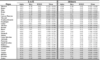
for h factor for each protocol-organ combination. The fitting parameters (α, β) and RMSE for h factor for the organs completely or partially inside the scan coverage with white background and for the organs outside the scan coverage with gray background are shown here. ... 19 Table 2.3. Fitting parameters (α, β) and root mean square from the residual for k factor for

each CT examination category. The fitting parameters (α, β), RMSE, and the mean value for k factor for the body CT examination categories with white background and for the neurological categories with gray background are shown here ... 24 Table 3.1. Estimated blood distribution in the vascular system, blood flow rate, and capillary

volumes used in PBPK standard contrast model. The compartments are numbered in the order that they appear in Figure 1. In our compartmental model, heart was constructed of three separate compartments: Left heart, right heart, and heart muscle. Note that due to the negligible amount of perfusion occurring in left and right heart, they were assumed as vessel compartments. The table only includes the organs’ names (except aorta) and the vessels are named with their compartment numbers (except aorta). ... 40 Table 4.1 Estimated blood distribution, blood flow rate, and capillary volumes used in the

standard forward model. The compartments are numbered in the order that they appear in Figure 1. In our compartmental model, the heart was constructed of three separate compartments: left heart, right heart, and heart muscle. Note that due to the negligible amount of perfusion occurring in the left and right heart, they were assumed as vessel compartments. The table includes the organs’ names and the vessels are named with their compartment numbers (except the aorta). ... 62 Table 4.2. Contrast material administration protocols. 32 different injection protocols

(12)

Table 4.3. The maximum value of the time-to-peak, peak-value, and mean absolute error results from both methods across the uni-phasic and bi-phasic protocols. ... 67 Table 5.1. Minimum, maximum, and mean values of the increase in CTDIvol normalized

organ dose (h factor) and DLP normalized effective dose (k factor) due to the administration of contrast medium with respect to the dose before injection. ... 83 Table 5.2. Mean and the standard deviation of the dose increase (in percentage) due to the

contrast medium. ... 88

(13)

List of Figures

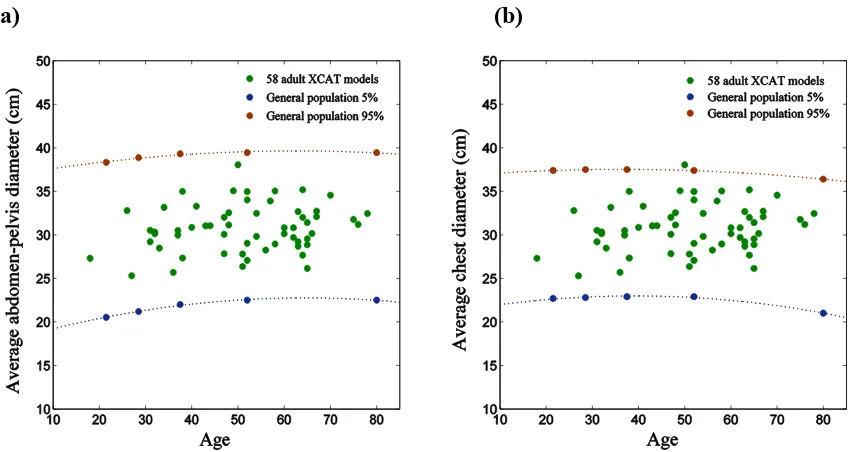
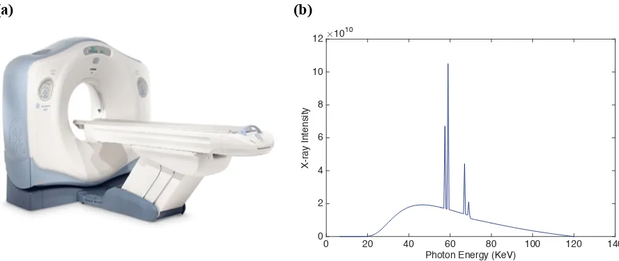
Figure 2.1. Variability in size among the patient models. The individual data points represent the average diameter of a) abdomen-pelvis and b) chest for 58 individual models, while lines represent the various (5 and 95 percent) percentiles according to general population-based studies (PeopleSize 2008, Open Ergonomics, UK). ... 9 Figure 2.2. a) A multi-detector array CT scanner LightSpeed VCT, GE Healthcare was used

in all simulations in this thesis. The scanner was equipped with 64 arrays/rows of detectors, allowing the user to select a beam collimation of 1.25–40 mm. The scanner can operate in both axial and helical scanning modes with a helical pitch of 0.516– 1.375. Three bowtie filters small, medium, and large were available on the scanner to provide size-adapted compensation for the variation of body thickness from the center to the periphery of the scan field-of-view (SFOV) in order to reduce dose and achieve more uniform x-ray intensity at the detector. The scanner automatically switched between a large and a small focal spot size based on tube current. The distance between the focal spot and the iso-center was 54.1 cm. The user could select a tube potential of 80, 100, 120, or 140 kVp. The detector of the scanner is consisted of 64 x 912 Ceramic Detectors. The slice thickness of 0.63, 1.25, 2.5, 3.75, 5, 7.5, 10 mm can be provided. The scanner enables up to 960 Scans per minute. The maximum scan time is 60 seconds. b) 120 kVp energy spectrum used in this study. ... 11 Figure 2.3. Probability that a given organ on the x-axis in a given CT examination category

on the y-axis is inside, on the periphery, or outside the scan coverage over the population of patients. ... 14 Figure 2.4. Organ dose plotted against average diameter of patient’s body inside the scan

coverage. Dose to the organs which are fully or partially irradiated in (a) liver scan; liver (as a large organ inside), adrenals (as a small organ inside), lungs (as an organ on the periphery), and bone (as a distributed organ), and (b) head-and-neck scan; brain (as a large organ inside), larynx and pharynx (as small organs inside), esophagus (as an organ on the periphery), and bone (as a distributed organ). ... 15 Figure 2.5. Organ dose plotted against distance between the center of the scan and the center

(14)

thyroid, larynx and pharynx, and bladder, and (b) head-and-neck scan; lungs, heart, and liver. ... 17 Figure 2.6. Effective dose for body and neurological CT examination categories. Effective

dose are plotted against (a) average patient’s body diameter for the body scan categories; chest, liver, and kidney, and (b) patient’s trunk length for neurological scan categories; head, neck, head-and-neck. ... 23 Figure 2.7. Comparison of dose to the liver after normalization by CTDIvol (h factor) across

five different protocols. ... 27 Figure 2.8. Comparison of organ doses after normalization by CTDIvol (h factor) in liver

scan. ... 27 Figure 2.9. Comparison of effective dose after normalization by DLP (k factor) (mSv per

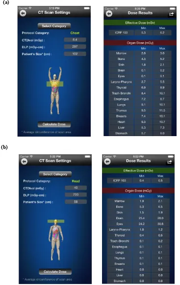
mGy-cm). ... 27 Figure 2.10. Screen captures of the Dose Calculator iPhone app showing a male adult patient

XCAT phantom in interactive rendering mode undergoing (a) chest and (b) head scans. ... 32 Figure 3.1. The physiologically based compartmental model used for simulating the

pharmacokinetics of contrast medium via the cardiovascular system through the body. The model includes 38 compartments: each ellipse represents a vessel compartment and each box represents an organ (see Table 3.1). ... 38 Figure 3.2. a) Organ and b) vessel compartments. Each organ is modeled by 3

sub-compartments: Intravascular, extracellular, and intracellular. CIV and CEC are intravascular and extracellular concentrations, and VIV and VEC are intravascular and extracellular volumes. Note that the input and output blood flow rates (Q) are assumed to be equal. ... 38 Figure 3.3. Collage of extended cardiac torso (XCAT) patient phantoms with variety of age,

size, gender, and anatomical diversity used in this study. ... 44 Figure 3.4. Intravenous contrast agent injection protocols. (Left) a uni-phasic injection of 125

mL of contrast material (320 mgI/mL) at 5 mL/sec and (Right) a bi-phasic injection of 50 mL of the same contrast agent at 2.5 mL/sec followed by 75 mL at 1 mL/sec. ... 46 Figure 3.5. Distribution of contrast material throughout a 5D XCAT model undergoing a

(15)

Figure 3.6. Iodine concentration curves for different organs (brain, heart, kidney, lung, liver, pancreas, small intestine, and stomach) used to update the particular organ’s material as a function of time in a male XCAT model. ... 49 Figure 3.7. Simulated and clinical aortic and hepatic contrast enhancement-time curves with

uni and bi-phasic injections. Simulated results are shown with thin solid cruves for the aorta (blue) and liver (red). The thicker black curves represent the mean value of simulation data for each data set. ... 50 Figure 3.8. Simulated contrast enhancement curves for different organs (brain, heart, kidney,

lung, liver, pancreas, small intestine, and stomach) across a library of 5D XCAT models undergoing a uni-phasic injection of 125 mL of contrast agent (320 mgI/mL) at 5 mL/sec. ... 51 Figure 3.9. Contrast enhancement curves for different organs (brain, heart, kidney, lung,

liver, pancreas, small intestine, and stomach) across a library of 5D XCAT models undergoing a bi-phasic injection of 50 mL of the same contrast agent at 2.5 mL/sec followed by 75 mL at 1 mL/sec. ... 52 Figure 3.10. Contrast enhancement calculator. ... 53 Figure 4.1. The physiologically based compartmental model used for simulating the

pharmacokinetics of contrast medium via the cardiovascular system through the body. The model includes 38 compartments: each ellipse represents a vessel compartment and each box represents an organ (see Table 4.1). ... 61 Figure 4.2. Iterative striping model. This figure summarizes the steps of the iterative

stripping technique. The unity signal strip, adjusted signal strip, and predicted uni-phasic injection function are shown at the top. The reference response, adjusted response functions, desired iodine concentration (calculated from the contrast enhancement), and subtracted reference function are shown below. ... 64 Figure 4.3. The enhancement curves calculated in the kidneys applying the analytical inverse

(16)

Figure 4.4. Error map created for the kidneys. The time-to-peak, peak value, and mean absolute errors in the prediction of the contrast enhancement in the kidney is based on the predicted injection functions applying the analytical inverse and iterative stripping methods across a) uni-phasic and b) bi-phasic injection protocols. Each block includes 16 different combinations of 4 iodine concentrations (y-axis) and 4 injection durations (x-axis). ... 68 Figure 4.5. Error bars created for different organs. The maximum value of errors in

prediction of the contrast enhancement based on predicted injection functions applying both analytical inverse (dark) and iterative stripping (light) methods across uni-phasic (left) and bi-phasic (right) injection protocols are shown for a) aorta, b) kidney, c) stomach, and d) small intestine. ... 69 Figure 4.6. Required injection function to achieve a desired enhancement in the kidneys

across our library of 58 XCAT models. Applying the analytical inverse method on a given contrast enhancement in the kidneys (solid line), different injection functions (dashed lines) were calculated for individual XCAT models. ... 72 Figure 5.1. Intra-venous contrast medium injection function. A uni-phasic injection function

of 125 mL of contrast agent (320 mgI/mL) at 5 mL/sec is shown. ... 77 Figure 5.2. Simulated iodine concentration curves for the different organs (spleen, liver,

kidneys, stomach, small intestine, large intestine, and pancreas) across a library of XCAT models undergoing a contrast-enhanced abdomen CT scan. ... 81 Figure 5.3. Monte Carlo simulation of the organ dose to the heart, spleen, liver, kidneys,

stomach, large intestine, small intestine, and pancreas as a function of time across the XCAT models undergoing a contrast-enhanced abdomen CT scan. The organ doses are normalized by CTDIvol. ... 82 Figure 5.4. Calculated effective dose as function of time across XCAT models undergoing an

abdomen contrast enhanced CT scan. The effective doses are normalized by DLP. ... 83 Figure 5.5. Distribution of the maximum dose increment (in percentage) in the heart, spleen,

(17)

was imaged in a Siemens (FLASH) CT scanner and computational models were imaged using a CT scan simulator modeling the geometry of a GE CT scanner. ... 95 Figure 6.2. 3D CNR surfaces (left) and contours (right) with respect to iodine concentration

and radiation dose for a) Mercury and b) 4 XCAT models (2 normal and 2 obese). ... 97 Figure 6.3. SR results calculated from 4 XCAT models (2 normal and 2 obese) using a) organ

dose, b) CTDIvol , c) organ dose without effect of iodine, and d) from Mercury phantom using CTDIvol. ... 98

(18)

List of Abbreviations

CT Computed Tomography

mSv MilliSievert

VCT Virtual clinical trial XCAT Extended cardiac torso

5D Five dimensional

IC Iodine concentration

RD Radiation dose

CTDI Computed tomography dose index DLP Dose length product

SSDE Size specific dose estimation

mGy Milligray

kVp Peak kilovoltage ROI Region of interest CNR Contrast to noise ratio IR Iterative reconstruction

PBPK Physiologically based pharmacokinetics

SR Sensitivity Ratio

MP Mean percentage

TP Time to peak

PV Peak Value

(19)

1. Background and Introduction

Dramatic improvements in medical image quality and diagnosis have been introduced over the last two decades. Such advancements, particularly in computed tomography (CT), have resulted in improvements in patient diagnosis and treatment, but they have also raised new challenges and concerns related to the population risk from radiation exposure. The recent national Summit on Management of Radiation Dose in CT indicated a strong consensus among experts and leaders for targeting low effective dose levels as low as 1 mSv or less. Such a goal greatly accentuates the significance of optimizing imaging applications in terms of image quality versus ionizing radiation dose.

1.1 Virtual clinical trials in Computed Tomography

(20)

1.2 Computational phantoms

Growing number of new CT technologies and challenges introduced by clinical trials, highlight the essence of virtual clinical trials (VCT’s) as an “all-time high”. Virtual clinical trials, which involve the use of computational phantoms and models of the imaging process, can offer a more efficient means to evaluate current and emerging imaging systems and methods. Such trials are being increasingly explored for imaging researches. [5-8] Through such studies, imaging protocols may be adjusted for individuals based on size or weight, and radiation dose levels can be more accurately assessed. VCT’s can further provide the only means with which to quantitatively evaluate or compare products from competing vendors.

(21)

1.3 Administration of contrast material in CT examinations

In clinical practice, the administration of contrast material is widely administered to improve the image quality and diagnostic sensitivity [16]. However, different institutions have different procedures in regards to contrast enhancement. For example, some institutions alter the amount of contrast material based on patient size and age while others do not. Overall, there is not a consistent, systematic administration technique across the different clinical practices. This leads to inconsistent enhancement across different patients [17-19]. Without factoring in patient-specific attributes, contrast-enhanced CT examinations can not be fully optimized in terms of scan timing, image quality, or radiation dose [20]. The design and optimization of new contrast material administration techniques properly orchestrated with the scan parameters (e.g. scan timing) requires an established relationship between contrast enhancement and the injection function. Knowing the dynamics of contrast material distribution, we can design injection protocols for different patients based on the desired contrast enhancements.

1.4 Impact of contrast material on dose and optimization results

(22)

evaluating and optimizing CT imaging technologies.

Finally, in order to conduct comprehensive evaluation and optimization studies in contrast enhanced CT imaging techniques, the effect of contrast material on image quality and radiation dose need to be taken into account. For such studies a library is essential in order to optimize CT technologies so as to achieve a diagnostic image quality while minimizing dose. They will provide a platform from which to evaluate CT technologies across a population of models as opposed to characterizations based on limited or overly simplistic models that are not indicative of clinical reality. Such a library allows us to build towards an integrated patient-specific optimization of contrast medium dose, radiation dose, and image quality together.

Therefore, there is a need to, first, study the patient-specific organ dose in absence of contrast material, and second, to develop more realistic computational patient models with the presence of contrast material enabling virtual clinical studies to evaluate CT imaging technologies and methods that involve contrast material, and third, to devise prediction techniques for contrast administration to design task- and patient-specific injection protocols across different patients, and finally, to study the relationship between image quality, radiation dose, and contrast does in the greater task of imaging dose management, consistent contrast enhancement, and image quality optimization.

1.5 Design and Objective of the Dissertation

(23)

and using that to develop a new generation of computational patient phantoms, 5D XCAT models with the fifth dimension representing contrast dynamics, and third, employing the contrast enhanced phantoms to calculate the patient-specific increase in organ dose due to the presence of contrast material, and fourth, predication of the patient-specific injection function to achieve the desired contrast enhancement in different organs and vessels for a given medical task, and finally, to investigate the interdependency of most important CT factors: image quality, radiation dose, and contrast does towards optimization or design of the new imaging protocols and administration techniques.

Previous version of XCAT phantoms were applied in Chapter 2 to compute patient-specific organ doses and effective dose conversion factors for a representative collection of routinely used un-enhanced CT protocols across a large number (58) of adult patient phantoms. The dose results from abdomen scan in this chapter were compared to the results from contrast-enhanced models in Chapter 4, to calculate the impact of contrast material on radiation dose. Based on the findings, the work included the development of an iOS application as a convenient calculator for providing reasonable estimation of organ and effective doses for adult patients undergoing CT examination.

(24)

To address the common inconsistency in the contrast material administration techniques and hence the contrast enhancement results from patients undergoing contrast-enhanced CT examinations, in Chapter 4, a step was taken further to develop and evaluate a strategy to determine the required contrast material injection function to achieve a desired contrast enhancement for specific organs and vessels. Two methods were developed, analytical inverse and iterative stripping, to predict the required contrast medium injection function to achieve a desired contrast enhancement in specific organs by incorporation of our physiologically based compartmental model of dynamics of contrast material distribution.

Application of iodinated contrast medium in contrast enhanced CT examinations is accompanied by increase in radiation dose. In Chapter 5, a method was developed to quantify the patient-specific organ doses for a representative, routinely used contrast-enhanced CT abdomen protocol by employing our 5D XCAT models along with Monte Carlo simulation to model the physics of radiation transport and absorption. The radiation dose was investigated as a function of time due to the contrast medium administration across a wide population of anatomies. The study further included the characterization of the physics of radiation absorption using Monte Carlo simulations in the presence of contrast media (See Appendix).

(25)

2. Patient-Based Estimation of Organ Dose for a

Population of Adult Patients

2.1 Introduction

Remarkable technological developments in computed tomography (CT) in the last four decades, especially after the introduction of helical CT technology in the late 1980’s,[22, 23] have made CT an essential medical diagnostic tool.[23] CT usage in the United States has been growing by 10 to 15% every year. The average effective dose per person in the United States has nearly doubled in the last three decades mostly, due to an increase in the number of CT examinations performed.[24] As a result, radiation dose from CT has become a subject of public attention. The number of publications focusing on radiation dose in x-ray CT has risen considerably in the last twelve years.[25] There is a need to more accurately estimate the radiation dose and associated risks to patients undergoing CT examination.

(26)

methods,[28] leading to organ dose databases [29] and CT dose software packages such as ImpactDose,[30] ImPACT CTDosimetry, CTDOSE (CT-Dose 2010),[15, 31] and VirtualDose. However, most of these approaches have been based on oversimplified stylized phantoms or a small number of adult phantoms.[31]

The purpose of this study was to compute patient-specific organ doses and effective dose conversion factors for a representative collection of routinely used CT protocols across a large number (58) of adult patient phantoms. Based on the findings, the work included the development of an iOS application as a convenient calculator for providing reasonable estimation of organ and effective doses for adult patients undergoing CT examination.

2.2 Methods

2.2.1 Patients and computer models

(27)

cage, gallbladder, spleen) within the CT images were segmented and modeled. The obtained segmented images were converted to three-dimensional non-uniform rational basis spline (NURBS) surfaces using a NURBS-based 3-D modeling software (Rhinceros, McNeel North America, Seattle, WA).[33] Remaining organs, not easily segmented or visible in the scan coverage, as well as head, neck, arms, and legs, were added by morphing organs from an existing extended cardiac-torso (XCAT) model developed from visible human data to fit the framework defined by segmented organs. The organ volumes were further scaled and matched to predictions based on the patient’s height, weight, and gender. The predictions were based on autopsy studies. [34, 35] Tissue composition of each organ and structure in the models was defined based on the elemental composition and mass density information tabulated in the CIRS manual. [35]

(a) (b)

Figure 2.1. Variability in size among the patient models. The individual data points represent the average diameter of a) abdomen-pelvis and b) chest for 58 individual models, while lines represent the various (5 and 95 percent) percentiles according to general population-based studies (PeopleSize

2008, Open Ergonomics, UK).

(28)

2.2.2 CT Protocols

Thirteen CT examination protocol groups, consisting of ten body categories and three neurological categories were selected based on existing protocols in use at our institution (Table I). All ten body categories shared the same set of scan parameters of tube voltage of

120 kVp, pitch of 1.375, beam collimation of 40 mm, and large body scan field-of-view per our routine clinical procedure. The scan parameters used for neurological categories were tube voltage of 120 kVp, pitch of 1, beam collimation of 20 mm, and head scan field-of-view per our routine clinical procedures. All thirteen protocols and the associated scan parameters were explicitly modeled in the Monte Carlo simulation.

Table 2.1. CT examination categories investigated in this study and the associated starting and ending anatomical landmarks of scan coverage

Simulated Scan Coverage Examination Category Start _{(1 cm above)} End _{(1 cm below)}

Chest-Abdomen-Pelvis Lung apex Inferior ischium

Chest Lung apex Lung base

Abdomen-Pelvis Superior liver Inferior ischium Abdomen Superior liver Superior iliac crest Body Pelvis Superior iliac crest Inferior ischium

Adrenals Superior adrenals Inferior adrenals Liver Superior liver Inferior liver Kidneys Superior kidney Inferior kidney Liver-to-Kidney Superior liver Inferior kidney Kidneys to Bladder Superior kidney Inferior bladder

Head Vertex of skull Scalp bottom

Neurological Neck C1 C7

Head-and-Neck Vertex of skull C7

2.2.3 Radiation Dose Estimation

(29)

slice CT system (GE Light-Speed VCT system) including helical and axial modes and the bowtie filters (Figure 2).[36] The simulation was previously validated in both cylindrical and anthropomorphic phantoms to agree with measurements within 1%-11% on average and 5%-17% maximum.

(a) (b)

Figure 2.2. a) A multi-detector array CT scanner LightSpeed VCT, GE Healthcare was used in all simulations in this thesis. The scanner was equipped with 64 arrays/rows of detectors, allowing the user to select a beam collimation of 1.25–40 mm. The scanner can operate in both axial and helical scanning modes with a helical pitch of 0.516–1.375. Three bowtie filters small, medium, and large were available on the scanner to provide size-adapted compensation for the variation of body thickness from the center to the periphery of the scan field-of-view (SFOV) in order to reduce dose and achieve more uniform x-ray intensity at the detector. The scanner automatically switched between a large and a small focal spot size based on tube current. The distance between the focal spot and the iso-center was 54.1 cm. The user could select a tube potential of 80, 100, 120, or 140 kVp. The detector of the scanner is consisted of 64 x 912 Ceramic Detectors. The slice thickness of 0.63, 1.25, 2.5, 3.75, 5, 7.5, 10 mm can be provided. The scanner enables up to 960 Scans per minute. The maximum scan time is 60 seconds. b) 120 kVp energy spectrum used in this study.

For a given protocol, the pertinent starting and ending points of scan for each patient model were computed. For helical scans (body protocols) the over-ranging length (required for data interpolation in helical reconstruction) was estimated to be 6.40 cm. [4] The total scan length

Photon Energy (KeV)

0 20 40 60 80 100 120 140

X-ray Intensity

#1010

(30)

for each examination was determined by adding the total image coverage to the over-ranging length.

To simulate each CT scan, 80 million photons were initiated and tracked through each patient’s phantom, resulting in relative errors within 1% - 4%. The dose to the organs was tallied from the deposited energy by the photons in each individual organ as a whole (as opposed to in individual voxels). The secondary electrons were assumed to be absorbed locally once they were generated. As the dose data were binned into (large) organs, the simplifying assumption regarding secondary particle absorption would not impact the results. The collision kerma estimator used can be categorized as a track-length estimator which keeps track of photon fluence track-length. Dose to the red bone marrow which was not explicitly modeled was estimated by tallying the volume-averaged photon fluence spectrum at each skeletal site and using the fluence-to-dose conversion coefficients of monoenergetic

photons in cancellous bone of skeleton.[2]A single active marrow dose was then calculated

as its skeletal average using the age-dependent fractional distribution of active marrow tabulated in ICRP 89. [2]

A given organ can appear in different locations with respect to the scan coverage in different patients. This location was categorized as being completely “inside”, “on the periphery”, or completely “outside” of the scan region for each patient. An average likelihood, 𝑃!"#$, was computed for each organ-protocol combination using

𝑃_!"#$ = !!"∙!! !!"#∙ !

!! !!"#∙ !

!!"!#$ ∙100%, (1)

(31)

the patients. In the dose analysis in this study, if the probability of an organ for being inside the scan field of view was less than 25%, the organ was considered to be outside the scan. If the probability was between 25% and 75%, the organ was considered to be on the periphery of the scan protocol. If the probability was greater than 75%, the organ was considered to be inside the scan protocol.

The estimated absorbed organ dose values were then weighted by the tissue weighting factors and summed to obtain the effective dose as

𝐸= !𝑤! 𝐻! , (2)

(2)

where 𝐻_!is the dose to organ T and 𝑤_!is the tissue weighting factor defined by ICRP publication 103. Dose to gonads was approximated as dose to testes or ovaries separately, thus computing effective dose as a patient specific construct. Breast dose was included in the calculation of effective dose for all the phantoms. The “remainder” tissues mean dose of each gender was calculated as the remainder dose.

The estimated organ values for each patient across the CT examination categories were normalized by CTDIvol to calculate the so called h factor. The CTDIvol was estimated from the technical reference manual of the GE LightSpeed VCT scanner using the tables of CTDI100 and technique adjustment factors. The DLP was calculated using the corresponding CTDIvol and total scan length for each examination protocols as

𝐷𝐿𝑃= 𝐶𝑇𝐷𝐼!"# ×𝑠𝑐𝑎𝑛 𝑙𝑒𝑛𝑔𝑡ℎ!"!#$ , (3)

(32)

to within 5%. The CTDIvol per tube current values used for the body and neurological CT protocols, 6.23 and 21 mGy/100mAs, respectively, were estimated based on 32-cm-diameter and 16-cm-diameter CTDI phantoms.

2.3 Results

2.3.1 Organ Dose

Figure 2 provides a summary of the geometry of the various protocols and the organs receiving dose in the protocols with respect to their location and the scan area. In general, as expected key organs are within the scan coverage in their associated anatomical categories. But that is not always the case, particularly for small organs.

Figure 2.3. Probability that a given organ on the x-axis in a given CT examination category on the y-axis is inside, on the periphery, or outside the scan coverage over the population of patients.

(33)

decreased exponentially with increasing average diameter of the patient’s body within the scan field of view (SFOV) corresponding to each CT examination (Figure 3) as

𝐻_! 𝑑_!"# =exp 𝛼_!𝑑_!"#+𝛽_! (4a)

and ℎ 𝑑_!"# = exp 𝛼_!𝑑_!"#+𝛽_! , (4b)

where 𝑑_!"# is the average diameter of the cross sections of the patient’s body within the scan coverage and 𝛼!, 𝛽!, 𝛼!, and 𝛽! are the fitting parameters. The average diameter was

calculated for each patient model as

𝑑_!"# = 2 _!"! , (5)

where 𝑉 and 𝑙 are the total volume and length of the scan coverage, respectively. (a) (b)

Figure 2.4. Organ dose plotted against average diameter of patient’s body inside the scan coverage. Dose to the organs which are fully or partially irradiated in (a) liver scan; liver (as a large organ inside), adrenals (as a small organ inside), lungs (as an organ on the periphery), and bone (as a distributed organ), and (b) head-and-neck scan; brain (as a large organ inside), larynx and pharynx (as small organs inside), esophagus (as an organ on the periphery), and bone (as a distributed organ).

(34)

organs was strongly dependent on the size and location of the organ. The correlation was generally strong for large organs that were entirely located inside the corresponding scan coverage (𝑟> 0.88); however, it was generally weaker for small organs inside the scan coverage ( 𝑟>0.68), for the ones on the periphery (𝑟 > 0.49), and for the distributed organs (𝑟 > 0.63) (Figure 3.a). The small organs that did not follow this pattern, i.e., the organs inside the scan coverage for which 𝑟< 0.68, were the breasts in chest and chest-abdomen-pelvis categories. The organs on the periphery that did not follow this pattern, i.e., the organs that were partially irradiated but had 𝑟 < 0.49 were the trachea-bronchi in liver, liver-to-kidney, adrenals, and kidney-to-bladder scans; the esophagus in liver and liver-to-kidney; the testes in abdomen-pelvis and pelvis; and finally the gallbladder in adrenals scan. The dose for the organs outside the scan coverage showed weaker correlation with patient size (𝑑_!"#) but strong correlation with the distance between the center of the organ and the center of the scan region. The organ dose (in mGy per 100 mAs) normalized by CTDIvol (h factor) decreased exponentially with increasing distance from the center of the scan region for each CT examination to the center of each organ outside the scan coverage (Figure 4.a) as

ℎ 𝐷 = exp (𝛼_!_!"#𝐷+ 𝛽_!_!"#), (6)

(35)

(a) (b)

Figure 2.5. Organ dose plotted against distance between the center of the scan and the center of the organ. Dose to the organs which are outside the scan region in (a) liver scan; thyroid, larynx and pharynx, and bladder, and (b) head-and-neck scan; lungs, heart, and liver.

(36)

category. Since CTDIvol was constant for a given protocol, the same held true after the organ dose was normalized by CTDIvol. For each protocol-organ combination, the fitting parameters (𝛼!, 𝛽!, 𝛼!"#, and 𝛽!"#), root-mean-square of residuals, and mean value of h

(37)

Table 2.2. Fitting parameters (α, β), root-mean-square from the residual, and the mean value for h

factor for each protocol-organ combination. The fitting parameters (α, β) and RMSE for h factor for

the organs completely or partially inside the scan coverage with white background and for the organs outside the scan coverage with gray background are shown here.

a: Chest and Liver protocols

Chest Liver

Organ Alpha Beta RMSE* Mean** Alpha Beta RMSE Mean

Marrow -0.06 0.90 0.03 0.375 ± 0.067 -0.05 -0.02 0.02 0.241 ± 0.045

Bones -0.05 1.15 0.05 0.625 ± 0.103 -0.04 0.26 0.04 0.351 ± 0.067

Skin -0.04 -0.02 0.02 0.251 ± 0.036 -0.02 -0.97 0.02 0.188 ± 0.022

Brain -0.06 -2.25 0.00 0.016 ± 0.004 -0.11 -1.53 0.00 0.001 ± 0.000

Eyes -0.09 -1.47 0.00 0.014 ± 0.004 -0.12 -1.30 0.00 0.001 ± 0.001

Larynx Pharynx -0.03 0.27 0.17 0.484 ± 0.166 -0.12 -0.51 0.00 0.016 ± 0.007

Thyroid -0.05 1.63 0.18 1.100 ± 0.229 -0.11 -0.27 0.01 0.032 ± 0.012

Trachea-Bronchi -0.06 2.03 0.11 1.236 ± 0.224 -0.01 -0.83 0.06 0.288 ± 0.063

Esophagus -0.07 2.06 0.09 1.074 ± 0.209 -0.02 -0.32 0.06 0.438 ± 0.069

Lungs -0.06 1.92 0.06 1.270 ± 0.197 -0.02 0.02 0.08 0.532 ± 0.085

Thymus -0.05 1.97 0.12 1.384 ± 0.232 -0.11 0.46 0.07 0.212 ± 0.080

Breasts -0.04 1.28 0.16 1.123 ± 0.196 -0.15 1.02 0.13 0.294 ± 0.198

Heart -0.06 2.12 0.08 1.335 ± 0.228 -0.04 1.05 0.11 0.887 ± 0.164

Liver -0.06 1.68 0.12 0.846 ± 0.179 -0.05 1.70 0.05 1.091 ± 0.204

Stomach -0.06 1.59 0.14 0.908 ± 0.189 -0.06 1.82 0.07 1.110 ± 0.224

Spleen -0.07 1.93 0.15 0.863 ± 0.214 -0.05 1.50 0.06 1.036 ± 0.181

Large Intestine -0.04 -0.73 0.05 0.146 ± 0.055 -0.05 1.17 0.08 0.634 ± 0.142

Adrenals -0.11 1.02 0.19 0.577 ± 0.211 -0.06 1.61 0.04 0.886 ± 0.178

Pancreas -0.02 -0.17 0.20 0.562 ± 0.201 -0.07 1.94 0.04 1.007 ± 0.223

Small Intestine -0.04 -0.7 0.06 0.157 ± 0.063 -0.06 1.63 0.13 0.800 ± 0.214

Kidneys -0.18 2.21 0.13 0.296 ± 0.162 -0.07 1.93 0.07 0.957 ± 0.224

Gallbladder -0.12 1.28 0.27 0.452 ± 0.314 -0.05 1.79 0.13 1.180 ± 0.248

Ovaries -0.12 -0.83 0.00 0.005 ± 0.002 -0.26 2.86 0.01 0.054 ± 0.038

Uterus -0.10 -1.66 0.00 0.004 ± 0.001 -0.25 3.02 0.01 0.043 ± 0.029

Vagina -0.11 -1.61 0.00 0.002 ± 0.001 -0.26 3.27 0.00 0.014 ± 0.009

Bladder -0.14 -0.24 0.00 0.002 ± 0.001 -0.24 2.45 0.01 0.023 ± 0.015

Prostate -0.14 -0.23 0.00 0.001 ± 0.001 -0.23 2.43 0.00 0.012 ± 0.009

Testes -0.10 -3.06 0.00 0.000 ± 0.000 -0.15 -0.55 0.00 0.002 ± 0.001

b: Liver-to-Kidney and Abdomen protocols

L-to-K Abdomen

Organ Alpha Beta RMSE Mean Alpha Beta RMSE Mean

Marrow -0.03 -0.38 0.02 0.256 ± 0.038 -0.04 -0.06 0.03 0.292 ± 0.049

Bones -0.03 -0.10 0.05 0.373 ± 0.062 -0.04 0.23 0.05 0.426 ± 0.074

Skin -0.01 -1.31 0.02 0.203 ± 0.018 -0.01 -1.07 0.02 0.225 ± 0.022

Brain -0.13 -0.85 0.00 0.001 ± 0.000 -0.13 -0.35 0.00 0.001 ± 0.000

Eyes -0.14 -0.20 0.00 0.001 ± 0.001 -0.16 0.97 0.00 0.001 ± 0.001

Larynx Pharynx -0.14 0.23 0.00 0.016 ± 0.007 -0.15 0.90 0.00 0.016 ± 0.007

Thyroid -0.13 0.35 0.01 0.032 ± 0.013 -0.14 0.84 0.01 0.031 ± 0.012

Trachea-Bronchi -0.01 -0.82 0.06 0.288 ± 0.063 -0.02 -0.74 0.05 0.284 ± 0.055

Esophagus -0.02 -0.31 0.07 0.440 ± 0.070 -0.02 -0.27 0.06 0.436 ± 0.070

Lungs -0.02 0.02 0.08 0.533 ± 0.085 -0.02 0.08 0.07 0.528 ± 0.079

Thymus -0.10 0.37 0.07 0.212 ± 0.080 -0.10 0.43 0.05 0.205 ± 0.056

Breasts -0.21 2.18 0.13 0.295 ± 0.198 -0.25 3.12 0.13 0.284 ± 0.187

Heart -0.04 1.05 0.11 0.889 ± 0.165 -0.04 1.07 0.11 0.885 ± 0.162

Liver -0.05 1.64 0.05 1.099 ± 0.198 -0.05 1.64 0.05 1.106 ± 0.202

Stomach -0.06 1.78 0.07 1.119 ± 0.221 -0.06 1.77 0.07 1.127 ± 0.224

Spleen -0.05 1.45 0.06 1.044 ± 0.176 -0.05 1.44 0.06 1.051 ± 0.178

Large Intestine -0.03 0.58 0.10 0.714 ± 0.127 -0.04 1.03 0.12 0.855 ± 0.166

Adrenals -0.05 1.52 0.03 0.902 ± 0.170 -0.05 1.51 0.04 0.914 ± 0.172

Pancreas -0.06 1.84 0.04 1.025 ± 0.214 -0.06 1.84 0.04 1.042 ± 0.218

Small Intestine -0.04 1.02 0.13 0.900 ± 0.175 -0.05 1.42 0.12 1.057 ± 0.206

Kidneys -0.06 1.70 0.05 1.005 ± 0.200 -0.06 1.69 0.04 1.031 ± 0.201

Gallbladder -0.05 1.69 0.13 1.195 ± 0.241 -0.05 1.71 0.13 1.215 ± 0.247

Ovaries -0.19 1.40 0.01 0.060 ± 0.020 -0.20 1.89 0.02 0.110 ± 0.037

Uterus -0.16 0.86 0.01 0.048 ± 0.017 -0.18 1.56 0.02 0.089 ± 0.033

Vagina -0.20 1.73 0.00 0.016 ± 0.006 -0.14 0.30 0.00 0.028 ± 0.008

Bladder -0.16 0.62 0.01 0.031 ± 0.012 -0.17 1.27 0.02 0.057 ± 0.022

Prostate -0.15 0.22 0.00 0.019 ± 0.007 -0.16 1.03 0.01 0.034 ± 0.014

(38)

c: Adrenal and Kidney protocols

Adrenal Kidney

Marrow -0.05 -0.52 0.02 0.125 ± 0.027 -0.05 -0.27 0.02 0.168 ± 0.037

Bones -0.05 -0.25 0.03 0.180 ± 0.039 -0.05 0.12 0.03 0.245 ± 0.055

Skin -0.03 -1.50 0.01 0.102 ± 0.013 -0.02 -1.29 0.01 0.147 ± 0.016

Brain -0.10 -3.24 0.00 0.000 ± 0.000 -0.12 -1.95 0.00 0.000 ± 0.000

Eyes -0.08 -3.98 0.00 0.000 ± 0.000 -0.10 -2.98 0.00 0.000 ± 0.000

Larynx Pharynx -0.10 -1.89 0.00 0.006 ± 0.002 -0.12 -1.00 0.00 0.005 ± 0.002

Thyroid -0.11 -1.35 0.00 0.011 ± 0.004 -0.12 -0.72 0.00 0.009 ± 0.004

Trachea-Bronchi -0.15 0.29 0.02 0.083 ± 0.033 -0.16 0.90 0.02 0.069 ± 0.029

Esophagus -0.08 -0.53 0.05 0.172 ± 0.056 -0.10 0.07 0.05 0.142 ± 0.053

Lungs -0.17 0.73 0.06 0.171 ± 0.076 -0.16 1.12 0.05 0.135 ± 0.060

Thymus -0.17 0.25 0.01 0.058 ± 0.022 -0.16 0.41 0.01 0.048 ± 0.018

Breasts -0.18 -0.26 0.03 0.050 ± 0.040 -0.20 0.77 0.03 0.040 ± 0.036

Heart -0.23 1.38 0.07 0.295 ± 0.143 -0.25 2.30 0.06 0.220 ± 0.107

Liver -0.07 1.95 0.09 0.798 ± 0.213 -0.08 2.13 0.14 0.789 ± 0.259

Stomach -0.07 2.01 0.09 0.912 ± 0.230 -0.08 2.17 0.13 0.903 ± 0.277

Spleen -0.05 1.42 0.07 0.887 ± 0.168 -0.06 1.62 0.07 0.906 ± 0.198

Large Intestine -0.02 -0.39 0.09 0.373 ± 0.089 -0.04 0.71 0.09 0.687 ± 0.126

Adrenals -0.06 1.56 0.04 0.730 ± 0.157 -0.06 1.51 0.04 0.794 ± 0.168

Pancreas -0.07 1.75 0.07 0.830 ± 0.193 -0.07 1.89 0.07 0.907 ± 0.222

Small Intestine -0.03 0.12 0.10 0.461 ± 0.111 -0.04 1.10 0.11 0.879 ± 0.169

Kidneys -0.07 1.68 0.09 0.710 ± 0.182 -0.06 1.66 0.05 0.955 ± 0.197

Gallbladder -0.04 0.95 0.24 0.911 ± 0.265 -0.05 1.68 0.15 1.093 ± 0.255

Ovaries -0.19 -0.03 0.00 0.015 ± 0.005 -0.23 1.49 0.01 0.060 ± 0.021

Uterus -0.15 -0.81 0.00 0.012 ± 0.004 -0.17 0.57 0.01 0.048 ± 0.018

Vagina -0.19 0.10 0.00 0.004 ± 0.002 -0.22 1.58 0.00 0.016 ± 0.006

Bladder -0.19 -0.03 0.00 0.007 ± 0.003 -0.20 0.98 0.00 0.030 ± 0.011

Prostate -0.16 -0.89 0.00 0.004 ± 0.001 -0.19 0.74 0.00 0.018 ± 0.007

Testes -0.13 -2.42 0.00 0.001 ± 0.000 -0.14 -1.13 0.00 0.003 ± 0.001

d: Chest-Abdomen-Pelvis and Abdomen-Pelvis protocols

CAP AP

Marrow -0.06 1.31 0.02 0.714 ± 0.116 -0.05 0.69 0.03 0.493 ± 0.078

Bones -0.05 1.75 0.06 1.185 ± 0.192 -0.05 1.15 0.05 0.784 ± 0.125

Skin -0.03 0.30 0.03 0.541 ± 0.054 -0.02 -0.33 0.02 0.392 ± 0.033

Brain -0.07 -0.59 0.00 0.016 ± 0.004 -0.12 0.16 0.00 0.001 ± 0.000

Eyes -0.08 -0.29 0.00 0.014 ± 0.004 -0.16 2.39 0.00 0.001 ± 0.001

Larynx Pharynx -0.06 1.47 0.16 0.486 ± 0.165 -0.13 1.57 0.00 0.015 ± 0.007

Thyroid -0.04 1.38 0.18 1.101 ± 0.229 -0.11 1.29 0.01 0.032 ± 0.012

Trachea-Bronchi -0.05 1.82 0.12 1.256 ± 0.226 -0.02 -0.64 0.05 0.285 ± 0.054

Esophagus -0.06 1.80 0.10 1.111 ± 0.208 -0.02 -0.15 0.06 0.439 ± 0.071

Lungs -0.05 1.72 0.07 1.304 ± 0.198 -0.03 0.12 0.07 0.531 ± 0.079

Thymus -0.05 1.75 0.13 1.398 ± 0.230 -0.09 1.23 0.05 0.204 ± 0.055

Breasts -0.03 1.17 0.16 1.134 ± 0.196 -0.21 4.56 0.13 0.282 ± 0.185

Heart -0.05 1.92 0.08 1.384 ± 0.229 -0.04 1.17 0.11 0.880 ± 0.163

Liver -0.06 1.91 0.07 1.209 ± 0.211 -0.06 1.75 0.07 1.117 ± 0.205

Stomach -0.06 2.00 0.08 1.215 ± 0.227 -0.06 1.84 0.10 1.124 ± 0.226

Spleen -0.06 1.77 0.08 1.131 ± 0.195 -0.05 1.54 0.08 1.059 ± 0.185

Large Intestine -0.05 1.83 0.06 1.244 ± 0.204 -0.05 1.73 0.05 1.230 ± 0.204

Adrenals -0.06 1.81 0.05 0.977 ± 0.183 -0.06 1.64 0.05 0.932 ± 0.175

Pancreas -0.07 2.04 0.07 1.092 ± 0.218 -0.06 1.96 0.07 1.052 ± 0.222

Small Intestine -0.06 2.01 0.07 1.283 ± 0.231 -0.06 1.88 0.06 1.256 ± 0.227

Kidneys -0.06 2.00 0.04 1.084 ± 0.206 -0.06 1.82 0.05 1.066 ± 0.202

Gallbladder -0.06 1.90 0.15 1.293 ± 0.254 -0.05 1.83 0.15 1.233 ± 0.257

Ovaries -0.07 1.97 0.06 0.911 ± 0.200 -0.06 1.76 0.07 0.905 ± 0.198

Uterus -0.07 2.07 0.07 1.000 ± 0.222 -0.07 1.91 0.06 1.003 ± 0.219

Vagina -0.07 1.86 0.06 0.942 ± 0.195 -0.06 1.53 0.06 0.946 ± 0.177

Bladder -0.06 1.88 0.10 1.031 ± 0.210 -0.06 1.73 0.09 1.010 ± 0.204

Prostate -0.07 1.80 0.06 0.839 ± 0.163 -0.06 1.58 0.05 0.834 ± 0.157

(39)

e: Kidney-to-Bladder and Pelvis protocols

K-to-B Pelvis

Marrow -0.06 0.74 0.02 0.382 ± 0.074 -0.06 0.57 0.01 0.280 ± 0.053

Bones -0.06 1.21 0.04 0.605 ± 0.117 -0.06 1.02 0.03 0.477 ± 0.089

Skin -0.03 -0.49 0.02 0.293 ± 0.030 -0.03 -0.66 0.02 0.232 ± 0.024

Brain -0.10 -1.95 0.00 0.000 ± 0.000 -0.10 -3.10 0.00 0.000 ± 0.000

Eyes -0.10 -2.04 0.00 0.000 ± 0.000 -0.10 -3.30 0.00 0.000 ± 0.000

Larynx Pharynx -0.12 0.03 0.00 0.005 ± 0.002 -0.10 -2.58 0.00 0.000 ± 0.000

Thyroid -0.11 0.17 0.00 0.010 ± 0.004 -0.12 -1.14 0.00 0.001 ± 0.000

Trachea-Bronchi -0.14 1.76 0.02 0.070 ± 0.029 -0.15 0.68 0.00 0.005 ± 0.002

Esophagus -0.10 1.17 0.04 0.145 ± 0.054 -0.13 0.24 0.00 0.009 ± 0.004

Lungs -0.14 2.05 0.05 0.137 ± 0.061 -0.15 0.84 0.00 0.008 ± 0.003

Thymus -0.14 1.43 0.01 0.048 ± 0.018 -0.18 1.39 0.00 0.003 ± 0.001

Breasts -0.18 1.99 0.03 0.041 ± 0.037 -0.19 1.19 0.00 0.002 ± 0.002

Heart -0.19 3.22 0.07 0.223 ± 0.108 -0.19 1.95 0.00 0.011 ± 0.005

Liver -0.08 2.14 0.17 0.807 ± 0.267 -0.31 4.13 0.01 0.059 ± 0.050

Stomach -0.08 2.20 0.17 0.919 ± 0.283 -0.28 3.89 0.02 0.067 ± 0.053

Spleen -0.06 1.74 0.08 0.920 ± 0.201 -0.20 2.08 0.01 0.052 ± 0.029

Large Intestine -0.05 1.73 0.05 1.197 ± 0.210 -0.07 1.74 0.12 0.765 ± 0.198

Adrenals -0.06 1.59 0.06 0.817 ± 0.169 -0.18 1.67 0.01 0.078 ± 0.033

Pancreas -0.07 1.96 0.10 0.938 ± 0.230 -0.24 2.95 0.02 0.116 ± 0.062

Small Intestine -0.06 1.88 0.06 1.236 ± 0.233 -0.07 1.69 0.15 0.738 ± 0.214

Kidneys -0.06 1.77 0.05 1.011 ± 0.199 -0.21 2.40 0.05 0.210 ± 0.096

Gallbladder -0.06 1.82 0.18 1.136 ± 0.273 -0.29 3.66 0.03 0.145 ± 0.178

Ovaries -0.07 1.84 0.06 0.881 ± 0.206 -0.07 1.77 0.07 0.875 ± 0.191

Uterus -0.07 2.00 0.05 0.960 ± 0.228 -0.07 2.07 0.04 0.985 ± 0.222

Vagina -0.07 1.72 0.09 0.698 ± 0.186 -0.06 1.78 0.05 0.928 ± 0.191

Bladder -0.06 1.75 0.10 0.952 ± 0.212 -0.06 1.86 0.08 1.010 ± 0.205

Prostate -0.06 1.37 0.07 0.708 ± 0.144 -0.06 1.60 0.04 0.826 ± 0.154

Testes -0.45 8.79 0.13 0.194 ± 0.165 -0.02 0.68 0.32 1.243 ± 0.323

f: Head and Head-and-Neck protocols

Head H & N

Marrow -0.03 -2.51 0.0024 0.053 ± 0.003 -0.03 -1.83 0.0050 0.102 ± 0.006

Bones -0.06 -0.86 0.0159 0.164 ± 0.019 -0.05 -0.44 0.0257 0.271 ± 0.029

Skin -0.03 -2.61 0.0040 0.045 ± 0.004 -0.04 -1.80 0.0070 0.082 ± 0.008

Brain -0.03 0.10 0.0329 0.702 ± 0.038 -0.03 0.14 0.0320 0.737 ± 0.038

Eyes -0.01 -0.14 0.0827 0.704 ± 0.082 0.00 -0.25 0.0853 0.730 ± 0.085

Larynx Pharynx -0.19 -0.38 0.0025 0.029 ± 0.005 -0.04 0.55 0.0518 0.867 ± 0.063

Thyroid -0.22 -0.15 0.0011 0.011 ± 0.003 -0.02 -0.13 0.1532 0.629 ± 0.152

Trachea-Bronchi -0.15 -1.26 0.0005 0.004 ± 0.001 0.04 -2.80 0.0454 0.126 ± 0.045

Esophagus -0.12 -2.07 0.0004 0.003 ± 0.001 0.01 -2.84 0.0226 0.073 ± 0.022

Lungs -0.13 -1.63 0.0002 0.002 ± 0.001 -0.15 0.61 0.0037 0.030 ± 0.009

Thymus -0.14 -2.10 0.0002 0.002 ± 0.001 -0.21 1.35 0.0035 0.032 ± 0.016

Breasts -0.15 -1.45 0.0004 0.002 ± 0.001 -0.32 3.72 0.0041 0.014 ± 0.018

Heart -0.12 -2.46 0.0001 0.001 ± 0.000 -0.16 0.32 0.0013 0.012 ± 0.006

Liver -0.11 -2.69 0.0001 0.000 ± 0.000 -0.12 -0.57 0.0006 0.004 ± 0.002

Stomach -0.11 -2.85 0.0001 0.000 ± 0.000 -0.14 -0.35 0.0006 0.003 ± 0.002

Spleen -0.12 -2.27 0.0001 0.000 ± 0.000 -0.13 -0.41 0.0006 0.004 ± 0.002

Large Intestine -0.10 -3.67 0.0000 0.000 ± 0.000 -0.10 -2.15 0.0002 0.000 ± 0.000

Adrenals -0.10 -3.59 0.0001 0.000 ± 0.000 -0.11 -1.45 0.0005 0.002 ± 0.001

Pancreas -0.10 -3.67 0.0000 0.000 ± 0.000 -0.13 -0.55 0.0004 0.002 ± 0.001

Small Intestine -0.10 -3.95 0.0000 0.000 ± 0.000 -0.13 -0.94 0.0001 0.001 ± 0.000

Kidneys -0.10 -3.77 0.0000 0.000 ± 0.000 -0.12 -1.24 0.0002 0.001 ± 0.001

Gallbladder -0.10 -3.84 0.0000 0.000 ± 0.000 -0.15 -0.12 0.0003 0.001 ± 0.001

Ovaries -0.10 -5.53 0.0000 0.000 ± 0.000 -0.10 -3.94 0.0000 0.000 ± 0.000

Uterus -0.10 -5.48 0.0000 0.000 ± 0.000 -0.10 -4.28 0.0000 0.000 ± 0.000

Vagina -0.10 -5.93 0.0000 0.000 ± 0.000 -0.10 -4.49 0.0000 0.000 ± 0.000

Bladder -0.10 -5.82 0.0000 0.000 ± 0.000 -0.10 -4.43 0.0000 0.000 ± 0.000

Prostate -0.10 -5.39 0.0000 0.000 ± 0.000 -0.10 -4.40 0.0000 0.000 ± 0.000

(40)

g: Neck protocol

Neck

Organ Alpha Beta RMSE Mean

Marrow -0.03 -2.29 0.00 0.058 ± 0.004

Bones -0.05 -1.26 0.01 0.131 ± 0.015

Skin -0.05 -2.25 0.00 0.043 ± 0.004

Brain -0.01 -2.48 0.00 0.066 ± 0.005

Eyes -0.24 -0.25 0.01 0.050 ± 0.007

Larynx Pharynx -0.04 0.59 0.05 0.849 ± 0.063

Thyroid -0.02 -0.11 0.16 0.610 ± 0.155

Trachea-Bronchi 0.03 -2.63 0.05 0.122 ± 0.045

Esophagus 0.00 -2.58 0.02 0.070 ± 0.022

Lungs -0.16 -0.40 0.00 0.029 ± 0.008

Thymus -0.21 -0.10 0.00 0.030 ± 0.016

Breasts -0.33 1.62 0.00 0.013 ± 0.016

Heart -0.16 -0.79 0.00 0.011 ± 0.005

Liver -0.12 -1.45 0.00 0.003 ± 0.002

Stomach -0.14 -1.30 0.00 0.003 ± 0.001

Spleen -0.13 -1.33 0.00 0.004 ± 0.002

Large Intestine -0.11 -2.47 0.00 0.000 ± 0.000

Adrenals -0.11 -2.16 0.00 0.002 ± 0.001

Pancreas -0.14 -1.40 0.00 0.002 ± 0.001

Small Intestine -0.13 -1.72 0.00 0.000 ± 0.000

Kidneys -0.12 -2.13 0.00 0.001 ± 0.000

Gallbladder -0.15 -1.27 0.00 0.001 ± 0.001

Ovaries -0.10 -5.18 0.00 0.000 ± 0.000

Uterus -0.10 -5.00 0.00 0.000 ± 0.000

Vagina -0.10 -5.27 0.00 0.000 ± 0.000

Bladder -0.10 -5.21 0.00 0.000 ± 0.000

Prostate -0.10 -5.13 0.00 0.000 ± 0.000

Testes -0.10 -5.22 0.00 0.000 ± 0.000

* Root-mean-square of the residuals (RMSE) represents the average discrepancy between the h factor values predicted by using the fitting function and the h factor values calculated for individual patient. It has the same unit as h factor or organ dose.

** Mean represents the average value of the h-factor calculated for individual organs across all the patients. It has the same unit as h factor or organ dose.

2.3.2 Effective Dose

For all body protocols, the correlation between the effective dose before and after normalization by DLP (in mSv per 100 mAs and mSv per mGy-cm, respectively) and patient size (averaged diameter of the patient’s body inside the scan coverage) could be well described by an exponential fit (Figure 5.a). The effective dose decreased exponentially with the patient size as

𝐸 𝑑_!"# = exp 𝛼_!𝑑_!"#+𝛽_! and (7a) and

𝑘 𝑑_!"# =exp 𝛼_!𝑑_!"# +𝛽_! , (7b)

(41)

neurological protocols, effective dose was slightly more strongly correlated with the measured trunk length of the patient than with the patient diameter. More specifically, the 𝑟

value of the correlation of effective dose with diameter for protocol head, neck, and head-and-neck were 0.41, 0.15, and 0.18 which improved to 0.46, 0.48, and 0.48, respectively, when trunk length was used as the correlation factor. The estimated effective dose after normalization by DLP (“k factor”) (in mSv per mGy-cm) decreased exponentially with increasing length of trunk (Figure 5.b) as

𝑘 𝐿_!"#$% =exp 𝛼_!"𝐿_!"#$%+𝛽_!" , (8)

where 𝐿!"#$% is the measured trunk’s length and 𝛼!" and 𝛽!" are the fitting curve parameters. The fitting parameters (𝛼!, 𝛽!, 𝛼!", and 𝛽!"), root-mean-square of residuals, and mean value of the k factor are reported in Table III.

(a) (b)

Figure 2.6. Effective dose for body and neurological CT examination categories. Effective dose are plotted against (a) average patient’s body diameter for the body scan categories; chest, liver, and kidney, and (b) patient’s trunk length for neurological scan categories; head, neck, head-and-neck.

(42)

Table 2.3. Fitting parameters (α, β) and root mean square from the residual for k factor for each CT

examination category. The fitting parameters (α, β), RMSE, and the mean value for k factor for the

body CT examination categories with white background and for the neurological categories with gray background are shown here

k factor

Protocol Alpha Beta RMSE* Mean**

Head -0.02 -6.25 0.0013 0.0011 ± 0.0001

Head-and-Neck -0.04 -4.65 0.0004 0.0028 ± 0.0004

Neck -0.05 -3.98 0.0006 0.0044 ± 0.0007

Chest -0.04 -2.52 0.0014 0.0211 ± 0.0028

Liver -0.05 -2.57 0.0018 0.0195 ± 0.0035

Liver-to-Kidney -0.05 -2.37 0.0014 0.0187 ± 0.0037

Abdomen -0.05 -2.49 0.0013 0.0177 ± 0.0034

Adrenal -0.06 -1.98 0.0016 0.0212 ± 0.0047

Kidney -0.07 -2.10 0.0018 0.0174 ± 0.0044

CAP -0.05 -2.56 0.0007 0.0157 ± 0.0025

Abdomen-Pelvis -0.05 -2.64 0.0009 0.0144 ± 0.0026

Kidney-to-Bladder -0.07 -2.35 0.0017 0.0135 ± 0.0033

Pelvis -0.06 -2.86 0.0009 0.0101 ± 0.0020

* Root-mean-square of the residuals (RMSE) represents the average discrepancy between the k factor values predicted by using the fitting function and the k factor values calculated from the organ dose values of individual patients. It has the same unit as k factor or effective dose.

** Mean represents the average value of the k factor calculated for individual patients. It has the same unit as k factor or effective dose.

2.4 Discussion

(43)

Using the dose results from a large library of retrospectively chosen patients from our clinical operation such that they represent a wide range of body types and age groups of adult males and females, enabled accurate estimation of organ and effective doses. Most importantly, due to the fact that the CTDIvol-normalized organ dose (h factor) and DLP-normalized effective dose (k factor) results are largely scanner-independent, they can be further applied to other CT systems with reasonable accuracy (<10% [39] and 15% according to our calculations). k factors may also be applied to tube current modulated scan with some discrepancy (<8%). However, these numbers are averaged across the entire population. For a given patient, this discrepancy can indeed be as large as 25%, consistent with our earlier report. [40] This is due

to the fact that when the individual discrepancies are averaged across the population, the case variability reduces the differences. These results indicate that as a first order approximation, as approached in this study, we can generalize across scanners. However, true patient specific organ dose calculations need to take the exact scanner into account. Furthermore, more work is needed to enable organ dose estimation with tube current modulation.

(44)

the testes to be inside the scan is only 29%. As such, while approximation can be made to generalize organ doses across patient, the actual dose for a specific patient can only be most accurately estimated with full knowledge of patient and scan geometry.

(45)

Figure 2.7. Comparison of dose to the liver after normalization by CTDIvol (h factor) across five different protocols.

Figure 2.8. Comparison of organ doses after normalization by CTDIvol (h factor) in liver scan.