On a multi-class queue with class dependent window-flow control

by

Raif O. Onvural H.G. Perras

Computer Science Department

Center for Communications and Signal Processing North Carolina State University

Raleigh, NC, 27695-8206, USA and

u.

Koerner

Department of Communication Systems Lund University

Box 118

8-22100 Lund, SWEDEN

CCSP-TR-88/17

Abstract

We consider a single server queue shared by N different classes of jobs. Class

i jobs arrive at the queue in a Poisson fashion with a class dependent rate. The total number of class i jobs allowed to wait in the queue is Wi, the window size of this class. A class i job that arrives to find Wi class i jobs in the shared queue is

forced to wait in an input queue. There is one input queue for each class. All classes receive the sameservice at the shared queue, which is exponentially distri-buted. We analyze the two-class model numerically. For more than two classes, we obtain an approximate decomposition algorithm that utilizes the two-class numerical procedure. Validation tests showed that the approximation procedure is fairly accurate.

One of the resource man agernent tasks which critically affects the perfor-rnance of computer communicat.ion networks is the flow control. i.e. the regula-tion of accepted traffic such that the network is not overloaded. Unless proper flow control is enacted, throughput of the network may significantly degrade below its optimum value. The principle of flow control is to shift congestion from the interior of the network to the points of admittance. The most widely known protocol to control the flow in a network is the window-flow control. The idea is simply to refuse admittance of new traffic when a certain number of messages in a region of the network is unacknowledged. The permissible upper bound of unack-nowledged messages is called the window size (cf. Reiser [6]).

multi-chain queueing networks of the product form tvpe to include mechanisms of state dependent lost and triggered arrivals.

The problem of analyzing multiple window control mechanisms can be for-mulated as a single or multi-class closed queueing network with population con-straints. The population constraint is imposed as follows: In the single class case, it is assumed that a subnetwork is subject to a population constraint. That is, only upto a predefined number of customers are allowed in the subnetwork. The remaining customers are queued in an input queue. In the multi-class case, for a particular subnetwork, each class (or a group of classes) has its own population constraint. These models have been analyzed approximately as closed queueing networks by several authors. A review of these approximations can be found in Thomasian and Bay [7J. The reader is also referred to Krzesinski and Teunissen [2] for a more recent approximation algorithm. We note that these models were originally developed for multiprogramming systems. They may not be suitable for modeling window-flow control mechanisms, which naturally give rise to open queueing networks. It is necessary, therefore, to develop open multi-class queue-ing networks with population constraints.

number of classes. A class i job that arrives to the network at a time that there are u'! jobs in the shared queue is forced to wait in an input queue. Let C': be the capacity of the input queue. ("1 can he finite or infinite ...-\. class i job waiting in the input queue is allowed to enter the shared queue only when a class i job departs from the network. There is one input queue per class.

Input Queues

At

_~.

Shared Queue

mG--.

AN

_~.

Figure 1: A multi-class open queueing model

Exact analysis of this model is rather difficult. In this paper. we analyze this

queueing; model n umer icailv and approximatelv. In particular. the two-class

model is analyzed numerically. For more than t\VO classes. \ve analyze the model

using an approximate decomposition algorithm which utilizes the two-class numerical procedure. In the following section, we describe the numerical pro-cedure. In section III, we present the approximation procedure and its validation. In section IV, we analyze the behavior of some performance metrics with respect to the arrival rates and window sizes. Finally, the conclusions are given in section

v.

II. The Queueing Model with Two Classes

Let us consider the queueing model described in section I with two classes. Let

(nt,n2)

denote its state where ni is the number of class i jobs in the network,

probability of being in state (nl'n2)' Seeing that the system under study is

n1

+

1 " ,

- - - - ,-J.LP(n17l.n~)T---J.LP(nt,n,!+1)

nl+w~ll nl+t.u~

and,

(~l

+

A~)P(O,O)

=

J.L(P(l,O)

+

P(O,l))

We note that in these equations, the probability of being in an infeasible state, i.e, ni

>

C,

+

wi' or ni

<

0, is equal to zero.

follows:

for i:=O to (w _t

+

It) do for j:=O to tw~-;- C~) do

begin

ind:=ind+1;

states( ind):=(i

.i)

end;

The generation of the rate matrix can be accomplished easily by going through the list of states and generating all feasible transitions for each state. In general, from an arbitrary state (nl,n2) there are four possible transitions to states

IS:

Once the rate matrix is set up, the steady-state queue length distribution can be obtained using a numerical technique such as power method, Gauss-Seidel method, etc.

III. The Approximation Procedure

lu this section. we present a decomposition procedure for the approximate

analysis of the N-<'lass queueing system shown in Figure 1. Below, we first

con-sider the case of finite capacity input queues, i.e.,

C,

<

x. i= I,...,~. The algo-rithm is then extended to the case of infinite capacity input queues in section 111.2. Finally, in section 111.3, both cases are validated and the time complexity of the algorithm is given.

III. 1. Finite Capacity Input Queues

Let us consider the N-class queueing model shown in Figure 1with parame-ters Ai' wi' J.L and C,

<

x, i=l,....N, with N>3. We decompose the N-class sys-tem into N two-class systems, the first class of which is the class under considera-tion and the second class is the aggregation of all other classes.

A.t

Figure 2: A two-class model

(:.-t be respectively the arrival rate. window size and capacity of the input queue of the aggregated class. In the original model. the total number of class A. jobs in the shared queue varies between zero and the sum of the window capacities of classes 2 to :\. Therefore, set

.V

W:t =

I

v.

&=2

We also set the arrival rate of class A jobs equal to the sum of the arrival rates of the individual classes, i.e.

Setting these values for AA and WA as shown above results in an overestimation of the number of class A jobs in the shared queue. The total arrival rate is equal

N

to AA =

2:

Ai as long as the total number of class A jobs in the shared queue is

i=2

less than min Wj. Once this limit is reached, then in the real system, jobs J=2,..,N

belonging to the class with the smallest window size may not enter the shared JV

queue. Clearly, this is not considered in the aggregate class with AA

=

2:

Ai and

1=2

N

WA

=

2:

Wi. We reduce the effect of overestimating the number of class A jobs in

i=2

the shared queue by fixing appropriately the capacity of the input queue of the aggregate class. The size of this input queue can be anything between zero and

f

C

i-For a given arrival rate A.AI the probability of having k jobs in the shared

i=2

balance the overestimation of the shared queue. L~.1 should be small. Accordingly~ we studied the following problem nurnericallv: Given the parameters of class 1,

v ~.

'\.t == ~ A_l, arid tL'.1

==

~ 1L'i what is (he value of Ct such that the marginal

pro-,_.)

~-"" 1=2

babilities of class 1 jobs are approximated with minimum error. Rather surpris-ingly, this numerical study suggested that C.₄

=

0,1 or 2. Although these values of CA do not always give the best approximate values, they are observed to be the best in most cases and they are never too far from the value of CA which

results in the best approximate values. This is true for a range of different values of the parameters of the queueing model.

Once we fix the parameters of the aggregate class, the resulting two-class model is solved numerically using the procedure given in section II. The steps of the algorithmare summarized as follows:

Step 1: Without loss of generality, consider class 1as the class under

considera-N

tion. Let the parameters of the aggregate class be as follows: WA

=

~ Wi'

i=2

if p<0.8 if 0.8<p

Step 2: Solve the two class network numerically to calculate the marginal queue length distribution of class 1.

III. 2. Infinite Capacity Input Queues

\Ve will now consider the ~-class model with (--:l='X, i=l ... .\'". and .\'~:3.

Let -;r(n) be the total number of jobs in the network without distinzuishinz

~ '='

between classes. Then. the following lemma is immediate by appealing directly to the steady-state equations.

Lemma: Consider an N-class queueing model as shown in figure 1with parame-ters 'Ai' Wi' C£, i=l, ...,~, and fJ.. Let Ci=x for all i. Furthermore, let

1T(n)

be the probability that total number of jobs in the network is n. Then

N

1T(n

-1)~ Ai

=

~1T(n) i

=

1

iV JV

where,

1T(O)=l-(

~Ai/f.L), (~ Ai/f.L)

<

1.

i=1 ~·=1

Hence, the system behaves like an

MIMI

1 queue if we do not distinguish between classes. In order to use the numerical procedure developed in section II, we should know the total capacity for each class, i.e. C..

+

wi. In the case of infinite capacity input queues, we obtain these values by first determining the

c"

total finite capacity,

C·,

such that ~".(n) is approximately equal to 1, where

n=O

c" .. I

~ 1T(n)=l-pC +1. In particular, we use the following procedure to calculate C .

n=O

jV I

Step 1: Let p=

2:

A.t·/~ with p

<

1, and let C = 1. i

=

1

Step 2: while l-p

c·

+l

<

0.99999 do

Once. C' is calculated, we apply the algorithm presented above for finite capa-city input queues assuming (-t:==Cf1 for all i.

III. 3. Time Complexity and Accuracy of the Procedure

The approximation procedure presented above decomposes the ~-class queueing system into N two-class systems. The number of states in each two-class system is B,=(

C,

+

wi)(2+WA).Hence, the total time complexity of the algorithm

to calculate the marginal probabilities of all classes is 0

[61

Bl ].

'rVe note that

the time complexity of the exact numerical procedure is 0

(()]1

(C

j

+

Wj ) )

3

].

App. I Proc (sec)

I

Numer ical

Proc (sec)

IL'1'".'U'."!

)

J

3 i (1.2.3)

I

(:.c,:c,:.c),9

I

12 l:3.2.-1) I :-3.3 I 9.6 : 3 (1,3.2) 9 (:c,:c,x),ll (2.3.4) I

I

I

I :389.9 19.2 I

:3 u.i.i) .) (4.4.-t) (2.2,2) I 6.1 I ·).:3

I

I

:

3 (1,1.1) 0 (8.8~8) (2.2~2) 93.-1 9.1

3

(1,2,3)

,..,~

(8,8,8)

(2.2,2) 120.2 12.5

3

(1,2,3)

12

(:C,x,x),8

(3.3,3)

i3.3 11.4

3

(1,1,1)

,.,I (':c,x.:c),9

(2.2,2)

113.2

6.3

4

(1,2,5,4)

18

(6,6,6,6)

(2,2,2,2)

719.5 12.1

4 (1,2,1,4) 15

(6,6,6,6)

(2,3,5,4)

656.4 21.1

Table 1: CPU times ofthe exact numerical procedure and the approximation procedure

IV. Performance Metrics

The performance metrics used in this analysis are defined as follows: Let

'IT

j(

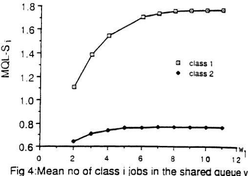
nj) be the marginal probability of having nj class i jobs in the network, l\tfQL - S, be the mean number of class i jobs in the shared queue, where

C·+w·

MQL -Sj =

'2:'

min(nj,wj) 'ITj(nj),

n,

=

1

MQL - I, be the mean number of class i jobs in the input queue, where MQL -

I

j

c.

2:

(nj-wd 'TTj(nj), and

T,

be the throughput of class i jobs, where

11.=Wi+1

if C·_I = : 0

otherwise

For the two-class model we study the behavior of MQL - Sj, l\tfQL - Ij , and

while all other parameters are kept the same. The values of these performance rnetrics are calculated numerically using the procedure described in section II.

Consider now the two-class model with parameters C'2=11. ,\1=2. A:!= l.

w2=2. and IJ.=-t. In figures 3 to ,5, W1 is varied from :2 to 11 while C1= 13-wI.

We observe that both ;,'"fQL - SL and ~\;[QL- S'?, increases as wI increases. As wI

increases, there are more class 1 jobs in the shared queue. This in turn reduces the rate at which class 2 jobs depart from the shared queue, thus increasing MQL - 52' As wI increases, there are less class 1 jobs waiting in the input queue,

hence MQL - II decreases. However, as the departure rate of class 2 jobs decreases, lwQL - 1₂ increases seeing that more jobs arrive to find W2 jobs in the

shared queue. For this example, both Ti's stay about the same as WI increases. Seeing that their values are very close to their respective arrival rates, we con-elude that the capacities of the input queues are as if they were infinite. We note that in this example Al

+

A2

<

J..L. Now, let us consider another example where

varied from 2 to 11 while CI=13-wt. In this case, all performance metrics are

{

13 - W

MQL -Ii

=

9 1

i=l i=2

J..L=7. and A~=l. In figures 9 to 11. ~\l is varied from l to 10. Increasing Al causes both .\[QL - .'31 and .\[QL - [1 to increase. as expected . .--\.s .Ir[QL - S1 increases.

the departure rate ofclass :2 jobs decreases. causing .\IQL - 52to increase slightly. This in turn causes ;.l;fOL - III_{... ...} to increase.

v.

Conclusions

We presented a model for the case where multiple connections use the same resource, depicted by a single server queue. .~ numerical procedure was imple-mented to calculate the steady-state joint queue length distributions. The number of states grows rapidly with the number of classes. In view of this, the numerical approach becomes infeasible even with a few classes. This necessitated the development of an approximation algorithm for more than two classes. The procedure decomposes the model to N two-class models, one for each class. Each two-class model is then analyzed numerically. Validation tests showed that the results are fairly accurate.

In

real situations, more than one node may be required to represent a virtual route. Furthermore, although the approximate procedure saves considerable amount of CPU time in the case of more than two classes, an accurate approxi-marion procedure for two-class model may result in even more savings. We are currently working on these two problems as an extension of the ideas presented in

0.6 w

o 2 4 6 8 10 121

Fig 4:Mean no of class i jobs in the shared queue

VS1

•

a class1

• class 2

~. 1.4 1.2 1.0 0.8

en

_I ....J

a

~

Fig 3: Throughput of class Ijobs vsw1

1.6

1 4

c class 1

1.2

•

class 1

1.0

•

•

•

0.8 .-1

1

0 2 4 6 8 10 ~2

Fig 6: Throughput of class Ijobs vsw1

1.0

0.8 c class 1

•

class2

0.6 I --1 _0.4

a

~ 0.2 0.0 wl

a 2 4 6 8 10 12

Fig 5:Mean no of class i jobs in the Input queue vsw1

1.6 ~-1.4 1.2 1.0 0.8 0.6 0.4

a 2 4 6 8

a class 1 • class2

10 12 10

.-en --l ₈

a

:E 6 4

2 a class 1

•

class 2

0 w

0 2 4 6 8 , a 12 1

Fig 7:Mean no of class i jobs in the shared queue vsw₁

12

10 class 1_class2

I 8 -J 0 ~ 6 4 2

o

w,

a 2 4 6 8 10 12

5

3

4

0;-c class 1 I

....J

3

•

Class2

_a

_{CJ c:ass 1}

~ 2

_•

_Class2

2

o

A

f

o 2 ~ 6 8 10 ~2

Fig 9:Througnput of class ijobsVS

A

4

o

A.

o 2 4 6 8 ~o 12

Fig 10:Mean no of class ijobs Inthe shared queue vs

Ai

10

8

--l

a

~

6

4 a class1

•

class2 2

o

A4

o 2 4 6 8 10 12

Fig 11:Mean no of class ijobs in the input queue vs

A

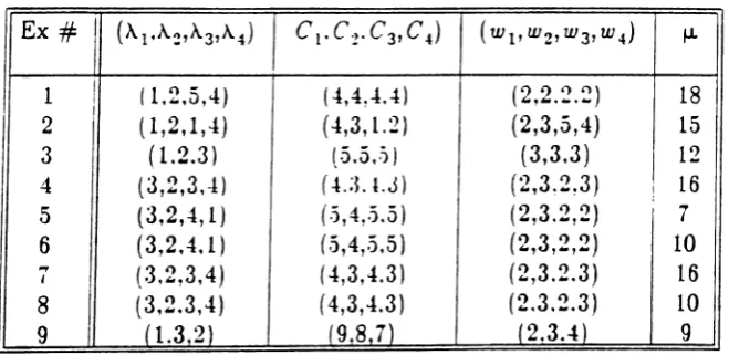
_f

Ex

#

(A.l·A~,A3,A.4) C1·C:?C 3,C.. ) (w1, wZ, w 3' w 4) f..I.

1 I ( 1,2,5,4) (4,4~-l.4) (2,2.~.~) 18 2 (1,2,1,4) (4,3,1.2) (2,3,5,4) 15

3 (1.2.3 ) (.5.5,,1) (3,3,3) 12

4 (3,2,3,-1 ) (-t.;LLJ) _{(2,3~2!3) !} 16

5 (3,2,4,1) (.),4,.5.5 ) (2,3.2,2) 7 6 (3,2,4,1) (,j,4"j,5 ) (2,3,2,2) 10

~

,

_{(3,2,3,4) (4,3,4.3)} (2,3.2.3) ₁₆

8 (3,2.3,4) (4,3,4.3) (2.3.2.3) 10

9 (1.3 2) (9.8,7) (2.3.4) 9

-0.00-r--...----r----...--r---~==!L_-..._l

0 2 3

class #

Fig 15: Relative error ~ for each classl (Example 4 in Table 2) \

I

•

mal-tOtal

0.80 a PrOb(O)

~ 0 \0-0 \0-0.60 \0-UJ CD :> ~ Q) _0.40 c: 020

•

au ~ 0.00

a 2 3 4

Class# i

Fig 13: Relative error JI _for

each _c1asl

-0

(Example 2 ; n Table 2 ) 0.70

0.60

~ _0.50

0

.... I

0 i \

.... ~

....

w 0.40 j

CD

.~ ~ I

(;i

0.30 &!I mqt-snlfld~

Q)

CI:

•

mqt-tataJ )Ii

0.20

•

Prob(O) ,_'~~

0.10

~

5 C rncr-snarec • mqf-total a Prob(O) 4 3 2 2 3 a~---"""-"""'-""'-"""-""-"""-""--"""-~ o Class # F:g 12: Relative error JI _for

each class

0

(Example 1 ; n Table 2 ) 0.70 .,

': 30i

"".,

l-i-O

~.30

.J.20

m mat-shared

0.10

_•

mqt-totaJ

II Prob(O)

-0.00

a 2 3 4

Class # Fig 14:Relative error 01 _for

each c 1as s

.D

(Example 3 ; n Table 2 )

15

2

O-t---.,.-..,...--...111=~-.--..-...-;;:.-....--,

a "~4 5

Class

#

Fig 17: Relative

error

% for each cl

(Example 6 in Table 2) 10

~ 8 m mqt-shared

0

' -

•

mqt-totaJ

0

...

a Prob(O)

' - ₆

w

CD > := 4 ~ Q)

a:

5 4 C mql-shared • mql-totaJ 3 2 5 Class #

Fig 16: Relative error ~ for each class (Example 5 in Table 2)

a-+---r--...

-~-

...-.,...--...--...-.---.

a

C mat-Sf • mqt-ta a Prob(C 4 3 2 Class #

o~-

....

-...-~...--

...-....,.-..,..-...-..,...--.---o a mql-shared • mql-totaJ • Prob(O) 4 5 3 Class# 2

o...

-...--~-...--~-....--

...- ...-..---...-.

o ~ 4 0

...

0

...

...

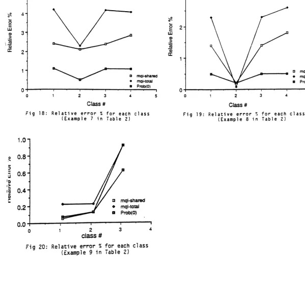
w Q) 3 .~ ,(; \ -Q) c: ₂

rig 18: Relative error % for each class

(Example 7 in Table 2) Fig 19: Relative(Example 8 in Table 2)error ~ for each class

1.0

0

0.8

~ ~

-

_0.6

u

11) l~ I~

0.4

D mql-shared t: m

0.2

•

mql-total

a Prob(O)

0.0

0 2 3 4

class

#

Fig 20: Relative

error

%

for each class

layered Window Flow Control vlechanisms ". Tech. Rep. Computer Science. 1988. North Carolina State Universit.y

[2] 4-\' Krzesinski and P. Teunissen , "Mult iclass Queueing .\"et\\"orks with Popu-lation Constrained Subnetworks". Proc ....\CYI SIG~1ETRICS Conf. on Measurement and Modeling of Computer Systems. .Austin. TX [August 1985), 128-139

[3] S.S. Lam, "Queueing .\:etworks with Population Size Constraints", IBNI .I.

Res. Develp., 370-378, July 1977

[4]

E.D. Lazowska and

J.

Zahorjan, "Multiple Class Memory Constrained Queueing Networks", Proc, ACM SIGMETRICS Conf. on Measurement and Modeling of Computer Systems, Seattle, W A (August 1982), 130-140

[5] M. Reiser, "A Queueing Network Analysis of Computer Communications Network with Window Flow Control", IEEE Trans. Comrn., vol, COM 27, 1199-1209, 1979

[6] M. Reiser, "Performance Evaluation of Data Communications Systems", Proc. IEEE, vol. 70, 171-196, 1982