Transactions of the 17th International Conference on Structural Mechanics in Reactor Technology (SMiRT 17) Prague, Czech Republic, August 17 –22, 2003
Paper # M02-1
Probabilistic Liquefaction Hazard Evaluation: Method and Application
James Marrone1), Farhang Ostadan2), Robert Youngs3), Joe Litehiser1)
1) Bechtel Corporation, San Francisco, California, USA
2) Bechtel National, Inc., San Francisco, California, USA
3) Geomatrix Consultants, Inc., Oakland, California, USA
ABSTRACT
Deterministic liquefaction potential evaluations are commonly made to assess the hazard from specific scenario earthquakes. These evaluations may assess the potential in a binary fashion (yes/no), or at best, define a factor of safety. More recent statistical analyses of liquefaction data have led to several models that predict the probability of liquefaction given a scenario event. In this paper a method is described that combines elements of a conventional probabilistic ground motion seismic hazard analysis with several new models for the conditional probability of liquefaction. This combination leads to a formal estimate of the annual probability of liquefaction that explicitly includes both uncertainties in regional seismicity parameters and in the conditional probability of liquefaction. The method not only allows calculating the composite liquefaction hazard from all seismic sources and their range of possible events, but, through deaggregation of the results, allows for assessing the relative contribution of various magnitudes, distances, or specific seismic sources. Example results are presented for sites in the San Francisco Bay Area (California).
The methodology presented is a robust probabilistic assessment of liquefaction potential, consistent with the current trend in U. S. regulations that require a probabilistic analysis of seismic hazards, such as U. S. Nuclear Regulatory Commission Regulation 10 CFR Part 100.23.
KEY WORDS: liquefaction, probabilistic, seismic hazard, earthquake, foundation design, ASHLE, SPT, cyclic stress ratio
INTRODUCTION
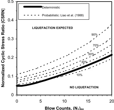
The traditional, and still most commonly used method for liquefaction evaluation of subsurface materials is deterministic ([1]; [2]; Figure 1). This method provides a binary – yes/no – determination of whether or not liquefaction will occur at a site. As it is applied to engineering design, and as depicted in Figure 1, the binary determinant is intentionally conservative, biased toward suggesting that liquefaction may occur. The margin against liquefaction is measured by determining a factor of safety based on “distance” from the binary determinant.
In recent years there has been the trend in engineering practice, as well as building code and critical facility regulations, to establish seismic design criteria in more robust probabilistic terms, including detailed specification of uncertainties ([3]; US Nuclear Regulatory Commission Regulation 10 CFR Part 100.23). While it is generally ground motions that are evaluated probabilistically, as in a probabilistic seismic hazard analysis (PSHA), a need often arises to evaluate the liquefaction potential itself within the context of a formal hazard analysis. For example, liquefaction potential may need to be measured against target performance goals for the facility, or to include explicit consideration of a range of possible local soil properties and regional seismic parameters.
0 0.1 0.2 0.3 0.4 0.5
0 5 10 15 20
Blow Counts, (N1)60
No
rm
alized
Cyclic S
tr
ess Ratio
(CS
R
N
) Deterministic
Probabilistic: Liao et al. (1988)
10% 30%
50% 70% 90%
LIQUEFACTION EXPECTED
NO LIQUEFACTION
Figure 1. Comparison of deterministic and
conditional probability assessment of
liquefaction hazard. In the 1980’s detailed statistical models of the occurrence of
liquefaction were developed to effectively allow the “distance” above or below the “yes/no” line of existing deterministic evaluations to be formally associated with a probability of liquefaction (see [4]; Figure 1). This probability of liquefaction was “conditional” in that it assumed that a given earthquake or earthquake ground motion had occurred.
both probabilistic ground motions and probability of liquefaction to be determined concurrently. Preprocessors of ASHLE allowed for determination of modeling (epistemic) or statistical (aleatory) variability of soil parameters to be incorporated into an ASHLE analysis, in concert with the variability of the seismic source parameters that is inherent in typical PSHA.
While robust, the ASHLE methodology was embedded within an existing PSHA computer code. Tt was not, therefore, able to provide probabilistic liquefaction potential predictions from previously calculated PSHA results. Subsequently, a variant of ASHLE, called ASHLES, was developed that performs the determination of liquefaction hazard as a post-process to the ground motion PSHA by using the PSHA ground motion hazard deaggregation matrices. ASHLES can be used, for example, in connection with the IPEEE studies for nuclear power plants [6].
The specific application of ASHLES demonstrated here is for the site in the San Francisco Bay Area, California, of another critical, although transportation rather than nuclear, facility.
METHOD
The program ASHLES predicts liquefaction hazard by calculation of the joint probability of the seismic ground motion hazard and the conditional probability of liquefaction at a specified location. This is performed as a post-process to the seismic ground motion hazard evaluation, using commonly-available ground motion deaggregation matrices (contribution to the hazard by binned magnitude and distance) for a suite of points (ground motion, annual probability of exceedance) along a ground motion hazard curve. The program allows incorporation of the variability or uncertainty of the standard penetration test results as a measure of cyclic shear strength resistance of the foundation soils.
Terms and Definitions:
To describe the theory and implementation of ASHLES, it is necessary to define a number of terms assumed units of measure.
Seismic ground motion hazard, P[Ei]
Site-specific seismic ground motion annual probability of occurrence of event Ei. For a conventional seismic hazard
evaluation, Ei is a minimum ground motion level - such as, a peak acceleration level of 0.5g - and P[Ei] represents the ith
point on the seismic hazard curve for the annual probability of exceedance of the specified ground motion type and level. ASHLES uses magnitude-distance deaggregation matrices of each point on a hazard curve for input of the seismic ground motion hazard.
Conditional probability of liquefaction, P[L|Ei]
Currently, ASHLES considers four published relations estimating the probability of liquefaction conditional upon the
occurrence of a given seismic event Ei at a specified “site” ([4]; [7]; [8]; [9]). The liquefaction potential is characterized by
the cyclic stress ratio as a measure of demand and the Standard Penetration Test as a measure of capacity.
Cyclic stress ratio, CSR
The cyclic stress ratio, CSR, is a measure of the seismic demand, expressed as equivalent uniform cyclic stress, divided by the initial effective overburden pressure. The average uniform cyclic stress ratio within a critical stratum at depth representative of the dynamic loading imposed by the earthquake is given by [10]:
d v v
EQ v
r
a ⋅ ⋅
⋅ =
' 0.65 max σ'
σ σ
τ
CSR= (1)
where
τ = average cyclic shear stress,
σv’ = effective vertical stress (psf) = buoyant density (pcf) * soil depth (ft)
amax = maximum ground surface acceleration (g)
σv = total vertical stress (psf) = total density (pcf) * soil depth (ft)
rd = nonlinear shear mass participation factor, also referred to as the depth-dependent stress reduction
coefficient
The maximum ground acceleration, amax, is a factor of the earthquake event, and is generally defined by the
The total (σv) and effective (σv’) vertical stresses are estimated from the geotechnical data available for a given site. The nonlinear shear mass participation factor, rd, is used to estimate accelerations, and therefore, the cyclic stress
ratio, at depth. Three of the four relations of conditional probability of liquefaction use a function of rd that is dependent
only on soil depth, while the relationship of Seed et al. (2001) uses an rd that is also a function of magnitude (M), amax, and
the average soil shear wave velocity of the upper 40 ft (Vs40). Alternatively, cyclic stress ratios can be obtained using shear
stresses developed from soil column analysis.
Normalized cyclic stress ratio, CSRN
For the purposes of assessing susceptibility to liquefaction, it is important to consider not only the severity of the
ground motion, as quantified by the ground motion acceleration, amax, but also the duration of shaking. Earthquake
magnitude, M, is an appropriate dependent variable for any functional parameterization of duration. For this purpose, [10] present a magnitude (7.5) normalized form of the cyclic stress ratio (CSRN):
m d
v v m
r r a
r = ⋅ ⋅ ⋅
= CSR / 0.65 max '
σ σ
CSRN (2)
where,
rm = earthquake magnitude scaling factor (MSF)
The factor rm adjusts for the lesser or greater number of cycles of ground motion that occurs during earthquakes of
magnitudes less than or greater than 7.5, respectively. This factor is inversely proportional to a power of magnitude, defined as unity for M = 7.5. ASHLES allows for various estimation methods of this parameter.
Standard Penetration Test, SPT
The Standard Penetration Test, SPT, is performed in the field to evaluate the penetration resistance of the granular soil, which is directly related to its liquefaction resistance. The measured blow count, N, is normalized to N1, which
represents the normalized penetration resistance of the soil under an effective overburden pressure of 1 ton per square foot.
(N1)60, used as a dependent variable in the conditional probability relations, is the corrected SPT resistance normalized to a
hammer energy ratio of 60% [11].
ASHLES allows for the uncertainty on measurements or estimates of (N1)60 to be incorporated into the liquefaction
probability evaluation through the definition of various types of distributions.
Numerical Operations
Given an evaluation of the probability of liquefaction occurring from a seismic event, P[L|Ei], and given the annual
probability that that seismic event occurs, P[Ei], we may estimate the joint probability, the annual probability of
liquefaction, by summing over all events Ei:
(3)
] [ ] | [ ]
[ i
i
i P E
E L P L
P =
∑
⋅Conventional seismic hazard evaluations consider the annual probability of exceeding a given ground motion level ‘a’:
P[ A > a] (4)
where ‘a’ may be peak ground acceleration. Actually, a hazard curve is defined by a discrete set of ai values, such that a
hazard curve is given as:
P[ A > ai] (5)
Basically, each point along the hazard curve is the composite contribution of all seismic sources as represented by modeled magnitude frequency or occurrence and spatial distributions. The uncertainty in the seismic input is modeled by considering various weighted contributions of different seismic model and ground motion attenuation parameters and/or their distributions. During the hazard calculation, the hazard contribution within specified magnitude intervals and distance intervals may be aggregated within accumulation bins, such that the hazard at a given ground motion (or corresponding
P[ A > ai | mj, dk] (6)
where mj and dk are representative central values of the magnitude and distance bins, respectively. It may be noted that:
(7)
∑
∑
>≈ >
k
k j i j
i P A a m d
a A
P[ ] [ | , ]
Literally, it is not appropriate to merely sum the probabilities. Instead, the appropriate summation is over the number of events of exceedance, which is then converted to a probability assuming a Poisson distribution. However, for hazards less
than about 10-3, the above summation is nearly numerically equivalent.
For the ASHLES methodology, there is no dependence on distance, so that the deaggregation over magnitude only is
used for each ground motion ai:
P[A>ai | mj] (8)
where
> ≈
∑
> (9)k i j k
j
i m P A a m d
a A
P[ | ] [ | , ]
Now, consider the hazard matrix given in Eq. 8. What is required for the liquefaction hazard estimate is the probability of a given ground motion level for which the conditional probability of liquefaction can be determined. Seismic hazard, however, is presented as a probability of exceedance. In fact, from fundamental probability theory, the probability of a given value of ground motion (or of any variable with a continuous distribution function at that value) is zero. What can be determined from the seismic hazard curve, however, is the probability of the occurrence of a ground motion level within a given interval, say between ai and ai+1:
P[ai+1>A>ai] = P[A>ai] - P[A>ai+1] (10)
The seismic hazard matrix, Eq. 8, that quantifies probability of exceedance, may be operated upon, as shown in Eq. 10, to develop a seismic hazard matrix that quantifies probabilities of ground motion intervals:
P[ai+1>A>ai|mj] = P[A>ai|mj] - P[A>ai+1|mj] (11)
In ASHLES we assume that the ground motion interval ai+1 > A > ai may be represented by a central value, āi, which we
define as the log mean of the bounding values, or
2 / )) ln( )
(ln( + +1
= ai ai
i e
a (12)
so that from Eqs. 11 and 12 a deaggregation matrix that represents an annual probability of occurrence is
P[A = āi|mj] ≡ P[ai+1>A>ai|mj] (13)
The ground motion āi is taken as amax and used as input into the CSRN function, and subsequently into the relation for
conditional probability:
P[L | CSRN(āi, mj,), (N1)60, . . . ] (14)
Therefore, from Eqs. 3, 13, and 14, the probability of liquefaction is the joint conditional probability of liquefaction given a seismic event and the annual probability of that event, summed over all events:
∑
⋅ ==
j i
j i j
i m N P A a m
a CSRN L P L P
,
60
1) ] [ | ]
( ), , ( | [ ]
[ (15)
Finally, where Eq. 15 indicates a single value of (N1)60, various distributions of (N1)60 may be considered. An additional
n n
j
i i j n i j
w m a A P N m a CSRN L P L
P =
∑
⋅ = ⋅,
, 1 60
] | [ ] } ) {( ), , ( | [ ] [ (16)
where wn are unity-normalized weights determined by the type distribution.
As stated before, there is no explicit dependence of conditional probability of liquefaction on distance, so as shown
in Eq. 9 we can sum over distance and work with a deaggregation array on magnitude. It may be of interest , however, to
retain the element of distance deaggregation if some source or spatial dependency on liquefaction hazard is to be evaluated.
For example, one might ask “Is the primary liquefaction hazard coming from a nearby or more distant source?” For this
reason Eq. 16 can be re-written to retain the summation over distance:
n n k j i k j i n j
i m N P A a m d w
a CSRN L P L
P =
∑
⋅ = ⋅, , ,
60
1) } ] [ | , ]
{( ), , ( | [ ] [ (17)
Suppressing the summation in Eq. 17 over either distance k or magnitude j, the relative contribution to liquefaction hazard
by distance or magnitude, respectively, can be determined.
APPLICATION
Current seismic hazard estimates for the San Francisco Bay Area have indicated that there is a 70% probability that a major earthquake on one of the major Bay Area faults, such as the Hayward or San Andreas faults, will occur within the next 30 years [12]. Even a more distant earthquake, such as the Ms=7.1 (Mw=6.9) Loma Prieta event some 90 km to the south, caused damage to the Oakland-San Francisco Bay Bridge and its feeder freeway system in 1989.
East Transbay Tube Ventilation Structure [TBTE]
0% 20% 40% 60% 80% 100%
5 6 7 8
Magnitude
Probabilit
y of Liquefaction Hayward
San Andreas
Method: Liao et al. (1988)
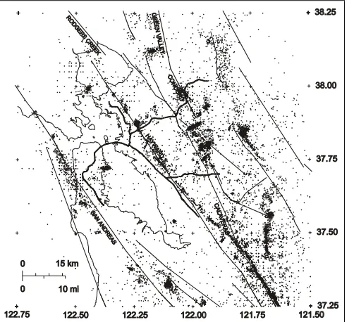
Figure 2. Map of the San Francisco Bay Area, showing earthquakes (ANSS); major faults (USGS), and the BART alignment.
Figure 3. Conditional probability of liquefaction for various scenario earthquakes.
One of the most critical elements of the BART system is the Transbay Tube that links the east and west sides of the bay. As part of the seismic retrofit program, the liquefaction hazard was also assessed using the methodology presented here.
Arango [14] performed a conventional deterministic liquefaction evaluation for the Project that suggested that fill materials surrounding the BART Transbay Tube are likely to liquefy during Bay Area maximum magnitude scenario earthquakes, specifically a magnitude 7.25 on the Hayward fault or a magnitude 8 on the San Andreas fault.
An assessment was made to quantify the conditional probabilities of liquefaction [Eq. 14] for the maximum magnitude scenario earthquakes, as well as a suite of smaller magnitude events along each of these major faults – as low as magnitude 5.0 – for various locations along the Transbay Tube. Figure 3 indicates that there is greater than a 50% probability of liquefaction along the Tube from a magnitude 6 or greater earthquake on the San Andreas or Hayward faults.
Finally, the ASHLES methodology was used to assess the joint annual probability of liquefaction from all magnitude events for all sources. This assessment is made for various locations along the BART Transbay Tube. Figure 4 shows the
Annual Hazard Curves: PGA
1E-05 1E-04 1E-03 1E-02 1E-01 1E+00
0 0.5 1 1.5 2
PGA (g)
Annual Frequency of
E
xceedance
TBTE: Rock, All Sources
TBTE: Soil, All Sources
TBTE: All Sources
Soil PGA: 0.539g Annual Hazard Level: 3.54e-03
Figure 4. Peak rock and soil acceleration hazard curves for all seismic sources for a Transbay Tube location [Eq. 5]. Circle symbols indicate the points along the hazard curve for which deaggregation matrices were available.
Figure 5. An example deaggregation matrix for one of the PGA hazard curve points (see Figure 4). This matrix
comprises one of the ith elements of Eq. 6.
rock peak ground acceleration (PGA) hazard curves for one of the locations. This figure also shows the corresponding soil PGA hazard curve, transformed from the rock curves using the soil/rock amplification relation presented in [15]. These soil PGA hazard curves correspond to Eq. 5. Each of the circle symbols on the hazard curve in Figure 4 indicates where a magnitude-distance deaggregation matrix value [Eq. 6] is available to use in ASHLES. Figure 5 is an example ground motion deaggregation matrix for one point along the hazard curve. As an observation for this particular site at this example ground motion and hazard level, the highest peaks are coming from the dominating contribution to ground motion hazard of the Hayward-Rodgers Creek (63%) and San Andreas (17%) faults, identifiable from their distinguishing magnitude and distance distributions. This deaggregation matrix indicates that much of the remaining PGA hazard contribution is coming from nearby (0 to 10km) smaller magnitude events not associated with any given fault. Deaggregation matrices for different points along a hazard curve will indicate differing relative contributions by the various seismic sources. As discussed above, and indicated by the summation over ai in Eq. 17, the evaluation of annual probability of liquefaction
Table 1 summarizes the results of the assessment of annual probability of liquefaction incorporating the contribution from all seismic sources for three sites along the Tube from east (TBTE) to west (TBTW).
Table 1: Annual Probability of Liquefaction
Site (N1)60Distribution Liao Toprak Youd Seed Average
TBTE 10 ± 3 7% 7% 6% 6% 7%
“ 14 ± 6 5% 6% 4% 5% 5%
TBTM 10 ± 3 6% 7% 6% 6% 6%
“ 14 ± 6 5% 6% 4% 5% 5%
TBTW 10 ± 3 6% 7% 6% 6% 6%
“ 14 ± 6 5% 6% 4% 4% 5%
The following conclusions from this application were made:
• The annual probability of liquefaction is on average 5% to 7% along the Transbay Tube.
• The east end of the Transbay Tube, has a very slightly higher (~1% higher) annual hazard of liquefaction than the
west end of the Tube.
• The range of estimated density of the backfill materials results in a difference of only 1% to 2% in annual
probability of liquefaction.
CONCLUSIONS
The methodology presented in this paper provides a robust approach for quantifying the probabilistic liquefaction hazard. The results of the seismic hazard studies can be incorporated in the methodology along with the site-specific soils data and its variation to evaluate the liquefaction hazard. This approach is consistent with the risk-aggregated approach currently used in the nuclear industry and finding increased application for other critical facilities. The method is most beneficial in decision making process for allocating limited funding for seismic upgrade of facilities constructed on poor soil conditions where foundation improvement can be very costly. The hazard evaluation provides a reasonable basis to determine the priorities for upgrading on the basis of the risk of the foundation failure.
REFERENCES
1. Seed, H. B., Arango, I., and Chan, C. K., Evaluation of Soil Liquefaction Potential for Level Ground During
Earthquakes, NUREG Report 0026, Nuclear Regulatory Commission, Washington, D.C., 1976.
2. Seed, H. B., Idriss, I. M., Arango, I., “Evaluation of liquefaction potential using field performance data”, J. Geotech.
Engrg., ASCE, Vol. 109, No. 3, 1983, pp. 458-482.
3. Senior Seismic Hazard Analysis Committee (SSHAC), “Recommendations for Probabilistic Seismic Hazard Analysis:
Guidance on Uncertainty and Use of Experts”, NUREG/CR-6372, Volume 1, U.S. Nuclear Regulatory Commission,
Washington, D.C., 1997.
4. Liao, S. S. C., Veneziano, D., and Whitman, R. V., “Regression models for evaluating liquefaction probability.” J.
Geotech. Engrg., ASCE, Vol. 114, No. 4, 1988, pp. 389-411.
5. Ostadan, F., Arango, I., Litehiser, J., Marrone J., “Liquefaction Hazard Evaluation”, Proc. of the 11th SMIRT
Conference, Tokyo, Japan, August 1991.
6. U. S. Nuclear Regulatory Commission, “Individual Plant Examination for Severe Accident Vulnerabilities--10CFR 50.54(f)”, Generic Letter 88-20, November 23, 1988.
7. Toprak, S., Holzer, T. L., Bennett, M. J., and Tinsley, J. C. (1999). “CPT- and SPT-based probabilistic assessments of
liquefaction potential”, Proc. of Seventh U.S.-Japan Workshop on Earthquake Resistant Design of lifeline Facilities
8. Youd, T.L., Idriss, I.M. Andrus, R.D. Arango, I., Castro, G., Christian, J.T., Dobry, R., Liam Finn, W.D.L., Harder, L.F., Jr., Hynes, M.E., Ishihara, K., Koester, J.P., Liao, S.S.C., Marcuson, W.F., III, Martin, G.R., Mitchell, J.K., Moriwaki, Y., Power, M.S., Robertson, P.K., Seed, R.B., Stokoe, K.H., II (2001). “Liquefaction resistance of soils: Summary Report from the 1996 NCEER and 1998 NCEER/NSF Workshops on Evaluation of Liquefaction Resistance
of Soils”, Journal of Geotechnical and Environmental Engineering, Vol. 127, No. 10, Oct. 2001, pp. 817-833.
9. Seed, R.B., Cetin, K. O., Moss, R. E. S., Kammerer, A. M., Wu, J., Pestana, J. M., and Reimer, M. F. “Recent
advances in soil liquefaction engineering and seismic site response evaluation”. Proc. of the Fourth International
Conference on Recent Advances in Geotechnical Earthquake Engineering and Soil Dynamics and Symposium in Honor
of W.D. Liam Finn, San Diego, CA, March 26-31, 2001.
10. Seed, H. B. and Idriss, I. M., Ground Motions and Soil Liquefaction During Earthquakes. Earthquake Engineering
Research Institute, Monograph Series, Richmond, CA., 1982, 134p.
11. Seed, H. B., Tokimatsu, K., Harder, L. F., and Chung, R. M. (1985). “Influence of SPT procedures in soil liquefaction
resistance evaluations”. J. Geotech. Engrg., ASCE, Vol. 111, No. 12, 1985, pp. 1425-1445.
12. Michael, A. J., Ross, S. L., Schwartz, D. P., Hendley, J. W., II, and Stauffer, P. H. (1999). Major quake likely to strike
between 2000 and 2030—Understanding Earthquake Hazards in the San Francisco Bay Region, U. S. Geological Survey Fact Sheet 152-99, 1999, 4 p.
13. Bechtel Infrastructure Corporation and The Bechtel/HNTB Team, BART Seismic Retrofit Program: Development of
BART Seismic Retrofit Design Ground Motion Criteria, San Francisco Bay Area Rapid Transit District, Oakland, CA.,
May 2002.
14. Arango, I., “Study on the vulnerability to seismic liquefaction of the fills around and below the Transbay Tube”, letter report for Bay Area Transit Consultants, Oakland, CA., February 2002.