ABSTRACT
WADDELL, CLEVELAND ALEXANDER. Parametric Linear System Solving with Error Correction. (Under the direction of Dr. Erich Kaltofen).
Consider solving a black box linear system,A(u)x =b(u), where the entries are polynomials in u over a field K, and A(u) is full rank. The solution, x = g(1u)f(u), where g is always the least common monic denominator, can be recovered even if some evaluations are erroneous. In [Boyer and Kaltofen, Proc. SNC 2014] the problem is solved with an algorithm that generalizes Welch/Berlekamp decoding of an algebraic Reed-Solomon code. Their algorithm requires the sum of a degree bound for the numerators plus a degree bound for the denominator of the solution. We describe an algorithm that given the same inputs uses possibly fewer evaluations to compute the solution.
We introduce a second count for the number of evaluations required to recover the solution based on work by Stanley Cabay. The Cabay count includes bounds for the highest degree polynomial in the coefficient matrix and right side vector, but does not require solution degree bounds. Instead our algorithm iterates until the Cabay termination criterion is reached. At this point our algorithm returns the solution. Assuming we have the actual degrees for all necessary input parameters, we give the criterion that determines when the Cabay count is fewer than the generalized Welch/Berlekamp count.
We then specialize the algorithm for parametric linear system solving to the recovery of a vector of rational functions, g(1u)f(u). If the rational function vector is the solution to a full rank linear system our early termination strategy applies and we may recover it from fewer evaluations than generalized Welch/Berlekamp decoding. We then show that if entries in our rational function vector are polynomials, then the vector can be viewed as an interleaved Reed-Solomon code. Thus if the errors occur in bursts we can again do better than generalized Welch/Berlekamp decoding.
The aforementioned algorithms do not work when the matrix of the system,A(u)x =b(u), is rank deficient and some evaluations cause errors. We next present an algorithm for solving black box linear systems where the entries are polynomials over a field and the matrix of the system is rank deficient. The algorithm first locates and removes all errors, after which it computes a solution that satisfies the input degree bounds.
©Copyright 2019 by Cleveland Alexander Waddell
Parametric Linear System Solving with Error Correction
by
Cleveland Alexander Waddell
A dissertation submitted to the Graduate Faculty of North Carolina State University
in partial fulfillment of the requirements for the Degree of
Doctor of Philosophy
Applied Mathematics
Raleigh, North Carolina 2019
APPROVED BY:
Dr. Terrence Blackman External Member
Dr. Ernie Stitzinger
Dr. Hoon Hong Dr. Kailash Misra
DEDICATION
To my grandfather the late Rev. Wilford Alexander Morris, my first formal teacher, his sister Zephreen Moriah for takig such good care of me as an infant. And to mother Bridget Marilyn
BIOGRAPHY
Cleveland Alexander Waddell, the last of my four children, the second of two boys, was born in 1987, September 28. His early education, Kindergarten - High School, was initiated and com-pleted in Guyana, South America, At the Pre-Kindergarten level he was ready and enthusiastic about attending school, especially the one his cousin was already attending. Pre-High School days, Cleveland is known to have been very playful yet evidenced a capability to balance play with sporting, church-related activities, and academic prowess.
It might be apt to say that Mathematics took a hold of him for classmates at high school sought his help with key concepts, he tutored students in his community, and he was decisive in his desire to pursue, abroad, a university level education and consequent qualification. Medgar Evers College afforded him such baccalaureate opportunity and he firmly grasped the challenge and honed his skill and aptitude in the Computer Science and Mathematics.That unwavering focus on scoring in cricket and basketball, and striding ahead of competitors in track events was applied to Graduate studies at North Carolina State University. The many Awards represent the acknowledgement and recognition of his scholarship.
Cleveland is, presently, part of a group that is promoting proficiency in Mathematics during the Summertime in Guyana. In his view, Mathematics could be fun. If my son had tutored me, I would have done better in Chemistry and Mathematics!
ACKNOWLEDGEMENTS
I wish to acknowledge the support by the National Science Foundation.
I would like to thank my adviser, Prof. Erich Kaltofen, for his problem, time and patience. This document would not be what it is without his guidance and support throughout the writing process. I would also like to express my gratitude to my committee members for sharing with me their wisdom and experience.
I would like to thank the academic support staff of the Department of Mahtematics during my tenure at the University for their help in ensuring all necessary administrative actions were taken in a timely manner. Your professionalism meant that I could focus my attention on finishing this document.
TABLE OF CONTENTS
List of Tables . . . vii
List of Figures . . . .viii
Chapter 1 Preface . . . 1
Chapter 2 Early Termination in Parametric Linear System Solving with Error Correction for Full Rank Systems . . . 4
2.1 Introduction . . . 4
2.2 Exact Vector of Function Solving . . . 7
2.3 Early Termination . . . 9
2.4 Cabay Early Termination . . . 14
2.5 Combined Early Termination . . . 20
2.6 Summary . . . 22
Chapter 3 Rational Vector Recovery with Error Correction as a Specializa-tion of Parametric Linear System Solving . . . 23
3.1 Introduction . . . 23
3.2 Rational Vector Recovery . . . 24
3.3 Cabay Early Termination with poles . . . 26
3.4 Summary . . . 28
Chapter 4 Parametric Linear System Solving with Error Correction for Rank Deficient Systems . . . 29
4.1 Introduction . . . 29
4.2 Exact Vector-of-Functions Solving - Rank Deficient Systems . . . 32
4.3 Removing Matrix Error . . . 36
4.3.1 The Algorithm . . . 45
4.4 Removing Right Side Vector Errors . . . 48
4.4.1 The Algorithm . . . 49
4.5 Returning a degree bounded solution in the Rank Deficient Case . . . 51
4.5.1 The Algorithm . . . 51
4.6 Summary . . . 52
Chapter 5 Polynomial Vector Recovery with Burst Errors . . . 53
5.1 Introduction . . . 53
5.2 Reducing the size of the system . . . 54
5.3 Summary . . . 63
Chapter 6 Modeling Polynomial Vector Recovery as a Burst Error Correcting Code . . . 64
6.2 Problem Description . . . 66
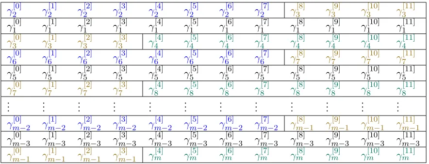
6.3 The Interleaving Scheme . . . 69
6.4 Data Transmission . . . 73
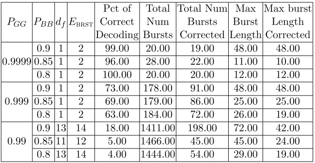
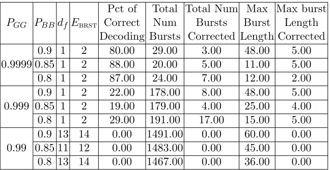
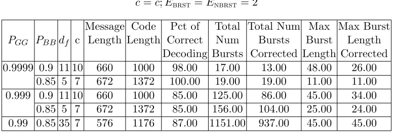
6.5 Performance on a Simplified Gilbert Channel . . . 76
6.5.1 Double Interleaving . . . 77
6.5.2 Experimental Results . . . 78
6.6 Summary . . . 82
Chapter 7 Conclusion . . . 83
Chapter 8 Future Work . . . 86
References. . . 88
APPENDIX . . . 90
LIST OF TABLES
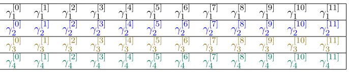
Table 6.1 Evaluated vectors before (m−1)Ebrst many evaluations are removed . . . 66
Table 6.2 Evaluated vectors after (m−1)Ebrst many evaluations are removed . . . . 67
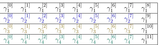
Table 6.3 Evaluated vectors to be transmitted . . . 67
Table 6.4 Evaluated vectors interleaved for transmission . . . 68
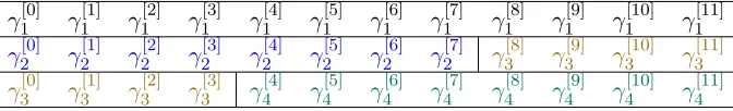
Table 6.5 Evaluated vectors interleaved for transmission . . . 74
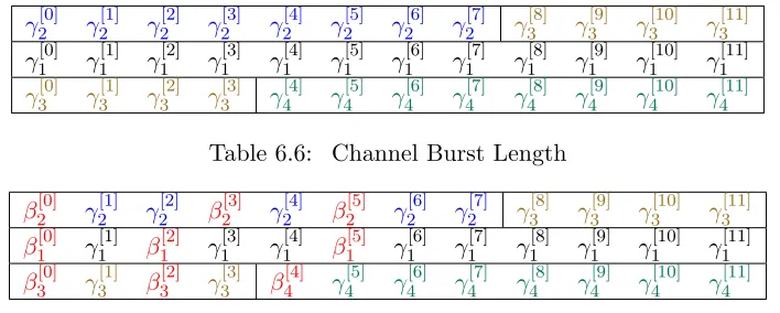
Table 6.6 Channel Burst Length . . . 74
Table 6.7 Evaluated vectors interleaved for transmission . . . 77
Table 6.8 Experiment Parameters . . . 78
Table 6.9 Stack + Burst Only + Minimal Interleave . . . 79
Table 6.10 Not Stack + Burst Only + Minimal Interleave . . . 80
Table 6.11 Stack + Burst Only + Not Minimal Interleave . . . 80
Table 6.12 Not Stack + Burst Only + Not Minimal Interleave . . . 81
Table 6.13 Stack + Not Burst Only + Not Minimal Interleave . . . 81
LIST OF FIGURES
Chapter 1
Preface
The need to store, compress and transmit digital data without the introduction of errors is as important today as it as ever been, if not more. If too many errors get into data then it may become corrupted, sometimes to the point where we can no longer gather useful information from it. While it is important to guard against errors, in some instances errors are inevitable. It may then be helpful to add redundant or parity data to the original data so that it can be recovered if errors are introduced. The process of adding redundant data so as to be able to recover the original data, if errors occur, is called error correcting codes. Error correcting codes is an essential tool in helping to mitigate the effects of noise and other issues that may introduce errors into data. They have been, and continue to be, used in a wide variety of applications from returning images from deep space, to ensuring clean crisp playback on optical disks. Big data analysis is a rapidly growing field of which the first step is to ”clean up” the data. Error correcting decoding will then be an essential tool for any data scientist. Given that successful communication requires unambiguity, exact solutions are required whenever possible. Thus, symbolic computation and computer algebra systems provide the best framework for doing error correction.
In January 2015 the author joined a research project that was focused on Parametric Linear System Solving with Error Correction. At that time the method being employed was a gen-eralization of the [Gemmell and Sudan 1992] description of the [Welch and Berlekamp 1986] decoder for [Reed and Solomon 1960] codes. The main results of the work done prior to the au-thor joining the research project can be found in [Boyer and Kaltofen 2014] Symbolic Numeric Computation (SNC) paper. The author along with collaborators continued the work presented in [Boyer and Kaltofen 2014]. The main results of the continuation along with the answers to some of the questions that were raised as result of continuing the work of [Boyer and Kaltofen 2014] are the subjects of this document (the author’s dissertation).
SNC paper. The algorithm computes the unique solution of a parametric linear system by first evaluating the system, then interpolating the parametric solution from the evaluation. See [McClellan 1973]. This algorithm is a generalization of the [Gemmell and Sudan 1992] description of the [Welch and Berlekamp 1986] decoder for [Reed and Solomon 1960] codes. The systems [Boyer and Kaltofen 2014] considered are full rank and overdetermined. The solution to such systems is a vector of rational functions. To enforce uniqueness, the solution is restricted to the one with the least common monic denominator. As mentioned in their SNC paper, there are two ways to view this algorithm. The first, and the main focus of the SNC paper, is numeric. That is the algorithm uses error correcting code techniques to account for ill-conditioned scalar matrices that result after the parametric systems have been evaluated. The second view is as a black box linear system solver that can correct true errors. True errors are scalar linear systems returned by the black box that do not agree with the evaluated solution. We will only consider the latter view in Chapter 2.
Chapter 2 continues with a description our early termination algorithms for parametric lin-ear systems solving with error correction. This work is published in the proceedings of the 2017 International Symposium for Symbolic and Algebraic Computation (ISSAC). See [Kaltofen, Pernet, Storjohann, and Waddell 2017]. As mentioned earlier the [Boyer and Kaltofen 2014] algorithm is a generalization of the [Gemmell and Sudan 1992] description of the [Welch and Berlekamp 1986] decoder for [Reed and Solomon 1960] codes. Thus this algorithm requires the sum of a degree bound for the numerators plus a degree bound for the denominator of the solution. It is possible that the degree bounds that are input to the algorithm are much larger than the actual degrees. We thus describe an algorithm, that given the same inputs may com-pute the solution from fewer evaluations. Later in Chapter 2 we introduce a second count that can be used to recover the solution of black box parametric linear systems with errors. This new count is based on the work by [Cabay 1971]. See also [Olesh and Storjohann 2007]. The Cabay count does not rely on degree bounds for the solution, rather it uses degree bounds for the parametric system. The algorithms iterates until the Cabay Criterion is reached. At which point it returns the solution. We then compare the two counts and say exactly when the Cabay count is fewer than the generalized Welch/Berlekamp count. Next we combine our two early terminations strategies into one general early termination algorithm. We also use an error rate as well as a rank drop rate instead of fixed bounds for the number of errors and rank drops respectively. This allows for further reduction in the number of queries to the black box. A similar strategy can be found in [Kaltofen and Yang 2013] and [Kaltofen and Yang 2014].
early terminations strategies apply. Thus we are sometimes able to recover the rational function vector using fewer evaluations than generalized Welch/Berlekamp decoding. If evaluations at poles (roots of the denominator) are allowed there are examples where the Cabay count is insufficient to recover the rational function vector. We show that if in addition to indicating that an evaluation is a pole the black box also gives information about the numerators of the solution then we are able to recover the solution.
In chapter 4 we describe an algorithm for parametric linear systems solving with error correction when the matrix of the system is rank deficient. Such systems have multiple solutions. We wish to compute a solution that agrees with the input degree bounds. In the full rank case the solution is unique and the solution of minimum degree has the error locator polynomial (a polynomial that has the error locations as its roots) as a factor. Unfortunately, this algorithm does not always return a solution that agrees with the degree bounds in the rank deficient case. The issue is that while the common monic denominator of minimum degree is unique there are many solutions with this denominator. The algorithm then does not always return a solution with the error locator polynomial as a factor. We know that if no errors occur the full rank algorithm works. The algorithm we describe for rank deficient systems first locates and removes the errors and we then able to compute a solution that agrees with the input degree bounds.
In the error model we used in Chapter 3 an errors means that one or more of the entries in the evaluated vector are wrong. While this model is reasonable, it is possible that errors affect the entire vector. We show in Chapter 5 that if errors affect the entire vector then we can solve an underdetermined system to find the solution and error locations simultaneously. We further show that if errors affect the entire vector then there is no need to assume that the erroneous values are random field elements.
In Chapter 6 we view the recovery of a vector of polynomials as the decoding of interleaved Reed-Solomon codes. It is known that interleaved schemes improve the error correction capa-bilities of codes when errors occur in bursts. See [Bleichenbacher, Kiayias, and Yung 2003] and [Schmidt, Sidorenko, and Bossert 2009]. We design a method for encoding a message as the coefficients of polynomials that is able to capitalize on the savings we describe in Chapter 5. We then test our technique on a Simplified Gilbert Channel, see [Yee and Weldon 1995], and present our initial findings
Chapter 2
Early Termination in Parametric
Linear System Solving with Error
Correction for Full Rank Systems
2.1
Introduction
Consistent linear systems of the formA(u)x =b(u), whereA(u)∈K[u]m×nand full rank,b(u)∈
K[u]m, m ≥ n, and K is a field, have as their solution rational functions xi = f[i](u)/g[i](u), 1 ≤i≤ n. In particular there is a solution g(1u)f(u),1 where g(u) is the monic, least common denominator, that is
GCD(f, g)
def
= GCD(GCDi(f[i]), g) = 1.
The solution of such a system can be determined by evaluating the system at distinct points ξ` ∈ K and interpolating the evaluated solution [McClellan 1973]. The solution can be found even if some evaluations are erroneous. The matrices of the systems we consider have full column rank, so their solution in the form g(1u)f(u) is unique. Note that for full rank matrices with univariate polynomial entries there are finitely manyξ`∈Kthat may cause the evaluated matrix to be rank deficient. If for each evaluation that causes the matrix with scalar entries to be rank deficient an extra evaluation is included, then techniques from algebraic error correcting codes can be used to compute the solution [Olshevsky and Shokrollahi 2003; Kaltofen and Pernet 2013; Kaltofen and Yang 2013, 2014; Boyer and Kaltofen 2014]. Furthermore in [Boyer and Kaltofen 2014] it is shown that for non-erroneous evaluation points, ξ`, it is not necessary to haveA(ξ`) andb(ξ`) in order to interpolate the solution. Rather it is enough to have a scalar
1
We write 1
gfiff is a vector of polynomials and
1
matrix ˆA[`] and right side vector ˆb[`] that have the evaluated solution g(1ξ`)f(ξ`) as a solution. Consider the following model. Suppose there exists an oracle, which we will refer to as the black box. If we supply the black box with a value,ξ`, from the fieldKthe black box returns to us ˆA[`] and ˆb[`]with entries from the fieldK. The scalar matrix, ˆA[`], and right side vector, ˆb[`], which are returned may not beA(ξ`) andb(ξ`). Nevertheless, if we query the black boxLtimes we assume that≤E times we get ˆA[λ]and ˆb[λ]such that ˆA[λ]f(ξλ)6=g(ξλ)ˆb[λ]. Such evaluations are considered to be erroneous. Furthermore we assume that fewer thanR times the black box returns ˆA[`] and ˆb[`] such that ˆA[`]f(ξ`) =g(ξ`)ˆb[`] but rank( ˆA[`])< n. The objective is to find the solution x = g(1u)f(u) of the system A(u)x =b(u) from as few queries of the black box as possible.
The count for the number ofξ`
L≥Lbk
def
= df+dg+R+ 2E+ 1 (2.1)
is employed by [Boyer and Kaltofen 2014] to recover the solution g(1u)f(u). The input parameters must satisfy the following specifications:
df ≥deg(f)
def
= max
1≤i≤m{deg(f
[i])}, dg ≥deg(g), (2.2)
E≥{λ|Aˆ[λ]f(ξλ)6=g(ξλ)ˆb[λ] for 0≤λ≤L−1}
,2 (2.3)
R≥{`|Aˆ[`]f(ξ`) =g(ξ`)ˆb[`]
and rank( ˆA[`])< n for 0≤`≤L−1}
. (2.4)
Here| · |denotes the cardinality of a set. The boundsE andRcan be derived from an error and singularity rate; see below. If n= m = 1 and ˆA[`] = I1 and ˆb[`] = g(1ξ`)f(ξ`) the algorithm is Welch/Berlekamp decoding of an algebraic (rational function) Reed-Solomon code [Welch and Berlekamp 1986]. We prove that for the vector rational function case if the input bounds in (2.2, 2.3, 2.4) are exact then the boundLbk is tight; see Lemma 1.
If the boundsdf anddg on input significantly overestimate the degrees, by early termination we can reduce the number of required evaluations to
L∗bk
def
= max{df + deg(g), dg+ deg(f)}+ 2E∗+R∗+ 1, (2.5)
where
E∗ ≥{λ|Aˆ[λ]f(ξλ)6=g(ξλ)ˆb[λ] for 0≤λ≤L∗
bk−1}
, (2.6)
R∗ ≥
{`|Aˆ[`]f(ξ`) =g(ξ`)ˆb[`]
and rank( ˆA[`])< n for 0≤`≤L∗bk−1}
. (2.7)
The number of evaluationsL∗bk in (2.5) is determined iteratively, without deg(f) and deg(g) as input, but has to meet the conditions (2.6, 2.7) for the number of erroneous and rank-deficient systems at evaluation points ξ`. One can use the estimate E∗ =E and R∗ =R from (2.3,2.4) before, but we will show in Algorithm 2 below how to dynamically adjust E∗ and R∗ from an error and singularity rate associated with the black box for ˆA[`],ˆb[`], as is originally suggested in [Kaltofen and Yang 2014, Remark 1.1].
Following Stanely Cabay’s [Cabay 1971] early termination strategy (see also [Olesh and Storjohann 2007]), we can derive a second count of number of evaluations. The new input parameters are specified as follows:
dA≥deg(A)
def
= max1≤i≤m,1≤j≤n{deg(ai,j)},
db ≥deg(b)
def
= max1≤i≤m{deg(bi)}.
(2.8)
Because in our algorithms we do not reconstructAand b, for the boundsdAanddb we can use that pair (A(u), b(u)) with A(u)f(u) =g(u)b(u) with a minimum deg(A). We derive a second evaluations count,
L∗cab = max{dA+ deg(f), db+ deg(g)}+ 2E∗+R∗+ 1, (2.9)
for recovering the solution. Here E∗ and R∗ bound from above the corresponding counts for erroneous and singular systems in (2.3, 2.4) withL∗cab replacingL∗bk. We prove that if all input parameter bounds are exact and deg(g)>deg(A) thenL∗cab< L∗bk.
2.2
Exact Vector of Function Solving
We describe and prove an early termination algorithm for the exact vector of function solving algorithm in [Boyer and Kaltofen 2014]. Their algorithm solves a system of linear equations
A(u)x =b(u) (2.10)
whereA(u) ∈K[u]m×n, b(u)∈K[u]m, m≥nand K is a field. The system is assumed to have a unique solution x = .. . 1
g(u)f[i](u)
.. .
∈K(u)n, g6= 0, (2.11)
where g is the monic least common denominator. If for all i, f[i] = 0 then g is set to 1. The solution vectorx is computed by:
1. SelectingL=df +dg+R+ 1 distinct elementsξ`∈K where
(a) 0≤`≤L−1 andξ`1 6=ξ`2 for`1 6=`2.
(b) df ≥deg(f). (c) dg ≥deg(g). (d) R≥
{`|rank(A(ξ`))< n= rank(A(u))} .
2. Solving the homogeneous linear system
A(ξ`) .. . Φ[i](ξ
`) .. .
−Ψ(ξ`)b(ξ`) = 0, (2.12)
where for all i,deg(Φ[i])≤ df and deg(Ψ)≤dg. The system (2.12) is linear in the coefficients of Φ[i](u) and Ψ(u). There aren(df + 1) +dg+ 1 unknown coefficients for Φ[i] and Ψ andmL equations.
Theorem 1 [Boyer and Kaltofen 2014] We suppose that for ≥ df +dg+ 1 of the ξ` we have rank(A(ξ`)) = rank(A(u)) =n. LetΨmin be the denominator component of a solution of (2.12)
with Ψmin 6= 0 and scaled to have leading coefficient 1 in u, and of minimal degree of all such
solutions, and let Φ[mini] be the corresponding numerator components of that solution. Then for alli we have Φ[mini] =f[i] and Ψ
The linear system (2.12) uses evaluations of A(u) andb(u) to solve forx = 1gf. The authors in [Boyer and Kaltofen 2014] show that it is not necessary to have the evaluations ofA(u) andb(u) in order to solve (2.10). Rather it is enough, for each ξ`, to have a scalar matrix ˆA[`] ∈Km×n and right side vector ˆb[`]∈Km such that ˆA[`]f(ξ`) =g(ξ`)ˆb[`].They also show that the solution can be computed even if some of the scalar matrices ˆA[`] and/or right side vectors ˆb[`] are erroneous. That is for some 0≤λ≤L−1,
ˆ
A[λ]f(ξλ)6=g(ξλ)ˆb[λ]. (2.13)
The solution is computed by:
1. SelectingL≥Lbk=df +dg+R+ 2E+ 1 distinct elementsξ` ∈K where
(a) R≥
{`|rank(A(ξ`))< n and ˆA[`]f(ξ`) =g(ξ`)ˆb[`],0≤`≤L−1}
, that is (2.4).
(b) E≥
{λ|Aˆ[λ]f(ξλ)6=g(ξλ)ˆb[λ],0≤λ≤L−1}
, that is (2.3).
2. Solving the homogeneous linear system
ˆ A[`]
.. . Φ[i](ξ`)
.. .
−Ψ(ξ`)ˆb[`]= 0, 1≤i≤m,0≤`≤L−1, (2.14)
where for all i,deg(Φ[i]) ≤ df +E and deg(Ψ) ≤ dg +E. The system (4.12) is linear in the coefficients of Φ[i](u) and Ψ(u). There aren(df +E+ 1) +dg+E+ 1 unknown coefficients of Φ[i](u) and Ψ(u) andmLbk equations.
Theorem 2 [Boyer and Kaltofen 2014]We suppose that for≤E of theξ` we haveAˆ[`]f(ξ`)6= g(ξ`)ˆb[`] and for ≥df +dg+E+ 1 of the ξ` we have rank( ˆA[`]) =n and Aˆ[`]f(ξ`) = g(ξ`)ˆb[`]. Let Ψmin be the denominator component of a solution of (4.12) with Ψmin 6= 0 and scaled
to have leading coefficient 1 in u, and of minimal degree of all such solutions, and let Φ[mini] be the corresponding numerator components of that solution. Furthermore, let Λ(u) =
Q
µsubj. to(2.13)(u−ξλµ) be an error locator polynomial. Then for all i we have Φ[mini] = Λf[i]
and Ψmin= Λg.
2.3
Early Termination
In the black box model it is not possible to determine degree bounds for the solution a-priori. Thus it is possible that the degree boundsdf anddgare much larger than max1≤i≤ndeg(f[i]) and deg(g) respectively. We describe next an algorithm that either finds the solution or determines that we need more evaluations. This allows us to design Algorithm 2, that computes the solution with possibly fewer evaluations than is required by the Lbk bound.
Algorithm 1: Compute 1gf and Λ or determine degree bounds are too small.
Input: df ≥deg(f),dg≥deg(g), 0≤df∗ ≤df, 0≤d∗g ≤dg, R∗ ≥{`|Aˆ[`]f(ξ`) =g(ξ`)ˆb[`]
and rank( ˆA[`])< nfor 0≤`≤L∗bk−1} ,
E∗≥
{λ|Aˆ[λ]f(ξλ)6=g(ξλ)ˆb[λ]for 0≤λ≤L∗
bk−1}
,
withL∗bk from Step 1 below,
a stream ( ˆA[`],ˆb[`]), ` = 0,1, . . . which is static on multiple calls and extensible in length on demand.
Output: 1gf and Λ or “deg(f)> d∗f and/or deg(g)> d∗g.”
1: L∗bk←max{df +dg∗, dg+d∗f}+R
∗+ 2E∗+ 1 2: Determine the null space of
ˆ
A[`]Φ∗(ξ`)−Ψ∗(ξ`)ˆb[`]= 0, `= 0,1, . . . , L∗bk−1, (2.15)
where deg(Φ∗)≤d∗f +E∗,deg(Ψ∗)≤d∗g+E∗
3: ifonly trivial solution then
return “deg(f)> d∗f and/or deg(g)> d∗g”; end if 4: Compute a basis,B, for the null space.
5: Compute the column echelon form for B,CEF(B). Retrieve the last column,
CEF(B)∗,r ←
−−−→ Ψ∗min −−→ Φ∗min[1]
.. . −−−→ Φ∗min[m]
,which has Ψ∗min 6= 0.
Here~· are coefficient vectors.
6: Λ∗ ←GCD(Φ∗min,Ψ∗min);k∗ ←deg(Λ∗).
7: (f∗, g∗)←(Λ1∗Φ∗min,Ψ∗min/Λ∗).
return “deg(f)> d∗f and/or deg(g)> d∗g”; end if 9: return f ←f∗, g←g∗,Λ←Λ∗;end if
Observe that Algorithm 1 is similar to the algorithm implied by Theorem 2. The main difference is that it uses the L∗bk≤Lbk count. Recall that Theorem 2 requires ≥Lbk evaluations to find
the solution. We use the results of Theorem 2 to prove the correctness of our algorithm. That is our algorithm either determines that we just computed an interpolant of the evaluation points or that we have indeed found the solution. Recall that we assume there exists a unique solution to equation (2.10).
In Step 2 we compute a solution similar to (4.12). The difference being that we use the starred bounds. Observe that if deg(f) ≤ d∗f and deg(g) ≤ d∗g and we were to substitute df =d∗f,dg =d∗g inLbk, then with L∗bk≥d
∗
f+d∗g+ 2E∗+R∗ by Theorem 2 we are guaranteed to find the solution (Λf,Λg). So ifB indicates there is only the trivial solution then it must be the case that deg(f)> d∗f and/or deg(g)> d∗g.
In Step 5 we compute a non-zero polynomial Ψ∗ of minimal degree (Ψ∗min 6= 0). We claim that the last column of CEF(B) contains Ψ∗min. The fact that the degree of Ψ∗min is minimum is clear from the form of the CEF(B). To see why Ψ∗min 6= 0, assume that Ψ∗min = 0. Then for allξ`, ˆA[`]Φ∗min(ξ`) = Ψ∗min(ξ`)ˆb[`]= 0m. On ≥max{df +d∗g, dg+d∗f}+E∗+ 1 evaluations rank( ˆA[`]) =n, that is Φmin∗ (ξ`) = 0, which implies by deg(Φ∗min)≤d
∗
f+E
∗ that Φ∗
min= 0. This
cannot be since CEF(B) is a basis for the solution space of equation (2.15) and thus cannot contain the zero vector. Hence Ψ∗min6= 0.
In Step 7 we define g1∗f∗ = Ψ∗1
minΦ ∗
min. We think of 1
g∗f∗ as our candidate solution. Next
in Step 8 we check if the candidate solution agrees with our starred bounds. We know from Theorem 2 that if d∗f ≥deg(f) and d∗g ≥deg(g) the bounds for the minimal solutions must be satisfied, so if they fail at least one bound is wrong.
Finally, we claim that if Algorithm 1 returns at Step 9 then we have computed the solution
1
gf. Of the L
∗
bk points ξ` at Step 9 we discard ≤ R
∗ “good” rank drops and ≤ E∗ erroneous
points for the solution (f, g) and ≤ k∗ = deg(Λ∗) ≤E∗ points ξ` that have Λ∗(ξ`) = 0. The remaining≥max{df +d∗g, dg+d∗f}+ 1 distinctξ` satisfy
1. rank( ˆA[`]) =n,
2. ˆA[`]f(ξ`) =g(ξ`)ˆb[`],
3. ˆA[`]f∗(ξ`) =g∗(ξ`)ˆb[`], because
ˆ
A[`]Φ∗min(ξ`) = ˆA[`]Λ∗(ξ`)f∗(ξ`)
and Λ∗(ξ`)6= 0.
From Items 2 and 3 we get ˆA[`](g(ξ
`)f∗(ξ`)−g∗(ξ`)f(ξ`)) = 0 which by Item 1 yieldsg(ξ`)f∗(ξ`)− g∗(ξ`)f(ξ`) = 0,that for at least max{df+d∗g, dg+d∗f}+ 1 distinctξ`. The vector (gf∗−g∗f)(u) has polynomials of degree ≤ max{df +d∗g, d∗f +dg} and is therefore equal 0, which proves
1
g∗f∗ = 1gf.
We observe thatd∗f ≤df and d∗g ≤dg implies thatL∗bk≤Lbk. Now Algorithm 1 guarantees
that with L∗bk many evaluations we either compute the solution 1gf or we determine that deg(f)> d∗f and/or deg(g)> d∗g. ThusL∗bk count can be used in an early termination strategy. We give the details in the following algorithm.
Algorithm 2: Early Termination Strategy.
Input: df ≥deg(f),dg≥deg(g),
ρE <1/2,a rational number with denominator qE, # the error rate.
ρR<1−2ρE,a rational number with denominator qR, # the rank drop rate, see Remark 2.
#qE =qR=∞ is permissible but may require # more evaluations.
Output: 1gf and Λ.
1: d∗f ←0;d∗g←0.
2: D←max{df+d∗g, dg+d∗f}+1.
3: E∗← bE¯∗c;R∗ ← bR¯∗c with
¯
E∗= 1
1−2ρE−ρR
ρE D+1− 1 qR
+(1−ρR) 1− 1 qE
. (2.16)
¯
R∗= 1
1−2ρE−ρR
ρR D+2− 2 qE
+(1−2ρE) 1− 1 qR
. (2.17)
4: ifAlgorithm 1(df, dg, df∗, d∗g, E∗, R∗) returns at Step 9
then return 1gf;end if 5: while(true)D←D+ 1.
# returns below forD= max{df+ deg(g), dg+ deg(f)}+1
6: Reassign E∗, R∗ as in Step 3 using the updated Din (2.16, 2.17).
7: for all(d∗f, d∗g) withD= max{df +d∗g, dg+d∗f}+ 1do 8: ifAlgorithm 1(df, dg, df∗, d∗g, E∗, R∗)
Remark 2 Algorithm 2 saves evaluations is two ways. The first way we save evaluations is by probabilistic computation ofE∗ andR∗ based on the size ofDrather than using fixed bounds. Like [Kaltofen and Yang 2013] we view evaluations as probing a black box, thus we can also relate the error rate of the black box toE∗. Also given the number of evaluation and a strategy for choosing the evaluation points one may have a rate at which the problem drops rank. Such a rate for the rank drop can then be related toR∗. If there is no such rate thenR from theLbk count can always be substituted forR∗ without affecting Algorithm 2.
We make the following assumption on the input error rates:
Assumption 1 Suppose that for L ≥LminE the number of erroneous evaluations, kE, always satisfies kE ≤ dρELe, and also for L ≥ LminR : kR ≤ dρRLe evaluations give rise to valid but rank deficient systems.
Here LminE andLminR are sufficiently large numbers of evaluations for which the assumptions onkE andkRare sensible. LetLmin = max{LminE , LminR }, thenLminis a minimum on the number
of evaluations our algorithm can work with. Assumption 1 differs from the rate assumptions in [Kaltofen and Yang 2013, Remark 1.1] and [Kaltofen and Yang 2014, Remark 1.1, Lemma 3.1] in that there we suppose kE ≤ bρELc, which implies no error for L <1/ρE. Our assumption here allows 1 error. Note that for ρR = 0,qR =∞ and ρE = 1/qE we get ¯E∗ =D/(qE−2) + qE/(qE−2) whereas in [Kaltofen and Yang 2013, 2014] we have ¯E∗ =D/(qE−2). In [Kaltofen and Yang 2014, Remark 1.1] the assumptions are probabilistically validated by adjusting the error rate upwards and bounding the probability of failure via Chernoff bounds.
We now show that Assumption 1 and the computation ofE∗andR∗in (2.16, 2.17) guarantee the input specifications for Algorithm 1. We have
¯
L∗ =D+ 2 ρEL¯∗+ 1− 1 qE
+ρRL¯∗+ 1− 1 qR
= 1
1−2ρE−ρR D+ 3− 2 qE
− 1 qR
and for ¯E∗,R¯∗ in (2.16,2.17) we have
¯
E∗=ρEL¯∗+ 1− 1 qE,
¯
R∗ =ρRL¯∗+ 1− 1 qR,
¯
Therefore we have
kE∗ ≤ dρEL∗bke=dρE(D+ 2E∗+R∗)e ≤ρE(D+ 2E∗+R∗) + 1− 1
qE ≤ρE(D+ 2 ¯E∗+ ¯R∗) + 1− 1
qE =ρEL¯∗+ 1− 1
qE = ¯E
∗
,
which implies by the integrality of kE∗ that k∗E ≤ bE¯∗c = E∗, as is required by Algorithm 1. Similarly, one provesk∗R≤R∗.
We discuss now the second way Algorithm 2 saves evaluations. The algorithm initializesd∗f and d∗g to zero. Thus L∗bk ≤ Lbk. The fewest number of evaluations we can use in Algorithm 1 is D+R∗+E∗ where D= max{df, dg}+ 1. Note this is the first bound used by Algorithm 2. We assume that D ≥ L, we can always adjust df and/or dg so that D ≥ L. If L∗bk has
2.4
Cabay Early Termination
We now describe the countL∗cab that incorporates degree bounds for the system being solved. The count is based on work in [Cabay 1971] (see also [Olesh and Storjohann 2007]). In The-orem 3, given exact values for degree parameters, we give the criteria and proof for when L∗cab < L∗bk.
Consider another count L∗cab,
L∗cab= max{dA+d∗f, db+d∗g}+R∗+ 2E∗+ 1,
wheredA≥deg(A) anddb ≥deg(b). See (2.8) for the definitions of deg(A) and deg(b). Similar to Algorithm 1 we present next an algorithm that uses the L∗cab bound and either determines one of the starred bounds is too small or returns the solution.
Algorithm 3: Cabay Early Termination
Input: dA≥deg(A), db ≥deg(b),
d∗f,d∗g,with 0≤d∗f ≤deg(f), 0≤d∗g ≤deg(g) # same as in Algorithm 1
R∗ ≥
{`|Aˆ[`]f(ξ`) =g(ξ`)ˆb[`]
and rank( ˆA[`])< nfor 0≤`≤L∗cab−1} ,
E∗≥{λ|Aˆ[λ]f(ξλ)6=g(ξλ)ˆb[λ]for 0≤λ≤L∗
cab−1}
,
Output: 1gf and Λ or ”deg(f)> d∗f and/or deg(g)> d∗g”.
1: L∗cab ←max{dA+d∗f, db+d∗g}+R∗+ 2E∗+ 1.
2: Determine the null space of the system
ˆ
A[`]Φ∗(ξ`)−Ψ∗(ξ`)ˆb[`]= 0, `= 0,1, . . . , L∗cab−1, (2.18)
where deg(Φ∗)≤d∗f +E∗,deg(Ψ∗)≤d∗g+E∗.
3: ifonly the trivial solution then
4: return deg(f)> d∗f and/or deg(g)> d∗g;end if 5: Compute a basis,B, for the null space
6: Compute the column echelon form for B,CEF(B).See Step 7 in Algorithm 1.
7: Λ∗ ←GCD(Φ∗min,Ψ∗min);k∗ ←deg(Λ∗).
8: (f∗, g∗)←(Λ1∗Φ∗min,Ψ∗min/Λ∗).
9: return f ←f∗,g←g∗, and Λ←Λ∗.
trivial solution then deg(f) > d∗f and/or deg(g) > d∗g. Assume deg(f) ≤d∗f and deg(g) ≤ d∗g. Then (Φ∗,Ψ∗) = (Λf,Λg) solves (2.18). Thus equation (2.18) cannot only contain the trivial solution. This implies that if (2.18) has only the trivial solution then deg(f) > d∗f and/or deg(g)> d∗g.
We now justify Step 9. We prove that g1∗f∗ is the solution of our system. Furthermore, the
GCD(Φ∗min,Ψ∗min) is the error locator polynomial. If we are at Step 9 of our algorithm then we have that on at least max{dA+d∗f, d∗g+db}+E∗+ 1 evaluations ˆA[`]f(ξ`) = g(ξ`)ˆb[`] and rank( ˆA[`]) =n. The latter implies thatg(ξ`)6= 0, for otherwisef(ξ`) = 0 and 1gf would not be reduced. For those `we have computed Φ∗ and Ψ∗ such that ˆA[`]Φ∗(ξ`) = Ψ∗(ξ`)ˆb[`].
We show first that ˆA[`]Φ∗(ξ`) = Ψ∗(ξ`)ˆb[`] implies A(ξ`)Φ∗(ξ`) = Ψ∗(ξ`)b(ξ`). If Ψ(ξ`) = 0 then Φ(ξ`) = 0 because ˆA[`] has linearly independent columns. If on the other hand Ψ(ξ`)6= 0 we get Φ∗(ξ`)/Ψ∗(ξ`) = f(ξ`)/g(ξ`) since the solution is unique. Now A(ξ`)(f(ξ`)/g(ξ`)) = A(ξ`)(Φ∗(ξ`)/Ψ∗(ξ`)) = b(ξ`). So the computed Φ∗ and Ψ∗ must satisfy A(ξ`)Φ∗(ξ`) = Ψ∗(ξ`)b(ξ`).
SinceA(u)Φ∗(u)−Ψ∗(u)b(u) is a polynomial vector of degree≤max{dA+d∗f, db+d∗g}+E∗ it is uniquely determined by max{dA+d∗f, db+d∗g}+E∗+ 1 distinct evaluation points so we have A(u)Φ∗(u) = Ψ∗(u)b(u). So 1gf = Ψ∗1
minΦ ∗
min = g1∗f∗. This implies there is a polynomial
Λ∗(u) with Λ∗f = Φ∗min and Λ∗g = Ψ∗min. For each λ we have ˆA[λ]f(ξ
λ) 6= g(ξλ)ˆb[λ] and ˆ
A[λ](Λ∗f)(ξλ) = ˆA[λ]Φ∗min(ξλ) = Ψmin∗ (ξλ)ˆb[λ] = (Λ∗g)(ξλ)ˆb[λ] which implies Λ∗(ξλ) = 0. Thus Λ = Λ∗.
Remark 3 Any non-zero solution computed in Step 5 of the previous algorithm has the prop-erty 1gf = Ψ1∗Φ∗. Nevertheless, only the pair (Φ∗min,Ψ∗min) = (Λf,Λg). So if there is no need to
compute the error locator polynomial then Step 6 is unnecessary.
Remark 4 If we implement Algorithm 2 replacing Algorithm 1 with Algorithm 3 then we then get an early termination strategy for Cabay Termination. 2
Remark 5 The matrix A(u) having full rank implies by Cramer’s rule that we can set df = (n−1)dA+db and dg =ndA. So Lcab ≥ndA+db+R+ 2E+ 1 =df +dg/n+R+ 2E+ 1 in comparison to Theorem 2, which has Lbk≥df+dg+R+ 2E+ 1. In Theorem 3 we generalize
when Lcab is better than Lbk.2
Theorem 3 If all bounds are exact then Lcab< Lbk if and only if deg(g)>deg(A).
Assume deg(g) + deg(b) < deg(A) + deg(f). Then Lcab = deg(f) + deg(A) +R+ 2E + 1 < Lbk= deg(f) + deg(g) +R+ 2E+ 1if and only if deg(g)>deg(A).
Now assume deg(g) + deg(b) = deg(A) + deg(f), then there are two cases. Case 1:Lcab= deg(f) + deg(A) +R+ 2E+ 1.
Case 2:Lcab= deg(g) + deg(b) +R+ 2E+ 1.
We have already dealt with case 1. Consider case 2, Lcab = deg(g) + deg(b) +R+ 2E + 1< Lbk= deg(f) + deg(g) +R+ 2E+ 1 if and only if deg(b)<deg(f). This implies deg(g)>deg(A) since we assumed that deg(g) + deg(b) = deg(A) + deg(f). 2
Remark 6 If n=m = 1 then the Cramer rule bound in Remark 5 yields, in the exact case, Lcab = Lbk. In fact the linear system A(u)x = b(u) is actually of the form a(u)x = b(u) where a(u), b(u) ∈ K[u]. This implies x = b(u)/a(u) = f /g which implies a(u) = h(u)g(u) and b(u) = h(u)f(u), where h(u) ∈ K[u]. Thus if we use the exact degrees for our bounds we get Lbk ≤ Lcab, since in this case deg(g) ≤ deg(A). Furthermore, if one uses fewer than L= deg(f) + deg(g) + 2k+ 1 evaluations then one loses the guarantee of a unique solution. In Lemma 1 below, given only L= deg(f) + deg(g) + 2kwe construct a second solution.2
Lemma 1 Let n=m= 1 andKa field. For allf, g∈K[u]withdeg(g)≥1andGCD(f, g) = 1 and for allξ0, . . . , ξL−1 withL= deg(f)+deg(g)+2k, ξ` 6= 0, ξ`1 6=ξ`2 for`1 6=`2,0≤`, `1, `2≤
L−1 and g(ξ`) 6= 0 for all ` with 0 ≤` ≤deg(f) + deg(g)−1 and for all k≥ 0 we have: if |K| ≥2(deg(f) + deg(g) +k) + 1 then there exist ¯f,g¯∈K[u]and there exist aˆ[`],ˆb[`]∈K for all ` with0≤`≤L−1 such that
1. f /g6=¯f/¯g, GCD(¯f,g) = 1,¯ deg(f) = deg(¯f) and deg(g) = deg(¯g). 2. ¯g(ξ`)6= 0 for all `with 0≤`≤deg(f) + deg(g)−1.
3. ˆa[`]f(ξ`) =g(ξ`)ˆb[`] for all ` with0≤`≤deg(f) + deg(g) +k−1, ˆ
a[`]¯f(ξ`) = ¯g(ξ`)ˆb[`] for all `with 0≤`≤deg(f) + deg(g)−1 or deg(f) + deg(g) +k≤`≤ L−1.
4. ˆa[`1]f(ξ
`1)6=g(ξ`1)ˆb
[`1] for all `
1 with deg(f) + deg(g) +k≤`1≤L−1 and
ˆ a[`2]¯f(ξ`
2)6= ¯g(ξ`2)ˆb
[`2] for all`
2 with deg(f) + deg(g)≤`2 ≤deg(f) + deg(g) +k−1.
Proof.Recall the system we solve is given by equation (4.12) and we solve ˆa[`]Φ(ξ`) = Ψ(ξ`)ˆb[`]. Let
Φ(u) =ydud+yd−1ud−1+. . .+y0 and
where d= deg(f) +k and e= deg(g) +k. For all `such that 0≤`≤deg(f) + deg(g)−1 let ˆ
a[`] =g(ξ`) and ˆb[`] =f(ξ`). Assume firstk= 0, i.e., there are no errors. We set up and solve the non-homogeneous linear system
ˆ
a[`]Φ(ξ`)−Ψ∗(ξ`)ˆb[`]= ˆb[`]ξe`, (2.19)
where Ψ∗ =ze−1ue−1+ze−2ue−2+. . .+z0.
Let B
"
y z∗
#
= v be the matrix representation of our system in (2.19). We have for the right side vector v that v 6= 0 since ˆb[`]= f(ξ`) cannot be zero for all 0 ≤`≤deg(f) + deg(g)−1 since deg(g)≥1 and ξ`6= 0 for all 0≤`≤L−1.Our system then has Lequations and L+ 1 unknowns, soB ∈KL×(L+1). By construction
"
f g∗
#
is a solution to our system. Since our system is underdetermined there must be other solutions
"
¯fc ¯ g∗c
# = " f g∗ # +cw
wherew 6= 0 is in the null space ofB andc6= 0. Letp= resu(f+cwf, g+cwg∗), pis a polynomial
inc, p6= 0 sincep(0)6= 0. Note deg(p)≤deg(f) + deg(g) and|K| ≥2(deg(f) + deg(g) +k) + 1. Thus there must be c1∈K such thatc1 6= 0, p(c1)6= 0 and lc(f)6=−lc(c1wf). Consider¯f =¯fc1
and ¯g= ¯gc1. Then by construction deg(f) = deg(¯f) and deg(g) = deg(¯g). Also sincep(c1)6= 0
we have that GCD(¯f,¯g) = 1.
Next we show that f /g 6= ¯f/¯g. We show first that
" f g∗ # and " ¯f ¯ g∗ #
are linearly
inde-pendent. Assume " f g∗ # and " ¯ f ¯ g∗ #
are linearly dependent, then there exits α 6= 0 such that
α " f g∗ # = " ¯ f ¯ g∗ #
, which implies α
" f g∗ # = " f g∗ #
+c1w, which further implies (α −1)
"
f g∗
#
=
c1w, α 6= 1 sincec1 6= 0 and w 6= 0.So αc−11
"
f g∗
#
=w, but 0 6= αc−1
1 v =
α−1
c1 B
"
f g∗
#
=Bw =
0, which is a contradiction. Thus
" f g∗ # and " ¯f ¯ g∗ #
are linearly independent, which implies that
" f g # , " ¯ f ¯ g #
are linearly independent. Which further implies thatf /g6=¯f/¯g.
To see why ¯g(ξ`) 6= 0 for all ` with 0 ≤ ` ≤ deg(f) + deg(g)−1, assume ¯g(ξ`) = 0 for all ` with 0 ≤ ` ≤ deg(f) + deg(g)−1. Since GCD(¯f,g) = 1 and ˆ¯ a[`]¯f(ξ`) = ¯g(ξ`)ˆb[`] then ¯
0≤`≤deg(f) + deg(g)−1.Thus ¯g(ξ`)6= 0 for all `with 0≤`≤deg(f) + deg(g)−1.
Now assume k > 0. By construction for all ` with 0 ≤ ` ≤ deg(f) + deg(g)−1 we have ˆ
a[`]f(ξ
`)−g(ξ`)ˆb[`] = 0 and ˆa[`]¯f(ξ`)−g(ξ¯ `)ˆb[`] = 0. Thus ˆa[`](¯g(ξ`)f(ξ`)−g(ξ`)¯f(ξ`)) = 0. Since ˆa[`]6= 0 it must be that ¯g(ξ`)f(ξ`)−g(ξ`)¯f(ξ`) = 0. Since f /g 6=¯f/¯g, and GCD(f, g) = GCD(¯f,g) = 1 then ¯¯ gf−g¯f ∈K[u] is not identically zero. Since deg(f) = deg(¯f) and deg(g) = deg(¯g) and (¯gf −g¯f)(ξ`) = 0 for all ` with 0 ≤ ` ≤ deg(f) + deg(g)− 1 we must have that deg(¯gf −gf¯) = deg(f) + deg(g). Observe that ξ` for 0 ≤ ` ≤ deg(f) + deg(g)−1 are deg(f) + deg(g) distinct roots of (¯gf −g¯f)(u), so (¯gf −g¯f)(u) can have no other roots. Let ˆ
a[`] = g(ξ`) and ˆb[`] = f(ξ`) for all ` with deg(f) + deg(g) ≤ ` ≤ deg(f) + deg(g) +k−1. Then for all `with 0≤`≤deg(f) + deg(g) +k−1 we have ˆa[`]=g(ξ`) and ˆb[`]=f(ξ`) and therefore ˆa[`]f(ξ`)−g(ξ`)ˆb[`]= 0.By construction ˆa[`]¯f(ξ`)−¯g(ξ`)ˆb[`]= 0 for all`with 0≤`≤ deg(f)+deg(g)−1.Let ˆa[`]= ¯g(ξ`) and ˆb[`]=¯f(ξ`) for all`with deg(f)+deg(g)+k≤`≤L−1 then have we have ˆa[`]¯f(ξ`)−¯g(ξ`)ˆb[`]= 0 for all` with deg(f) + deg(g) +k≤`≤L−1.
Assume there exist ξ` for some` with deg(f) + deg(g)≤`≤deg(f) + deg(g) +k−1 such that ˆa[`]¯f(ξ`)−¯g(ξ`)ˆb[`]= 0.Then (¯gf−gf¯)(ξ`) = 0 for thatξ`.Which is a contradiction since we have already shown that if ξ` is a root of (¯gf −g¯f)(u) then ` <deg(f) + deg(g). Thus for all ` with deg(f) + deg(g) ≤ ` ≤ deg(f) + deg(g) +k−1 we must have ˆa[`]¯f(ξ`) 6= ¯g(ξ`)ˆb[`]. A similar argument shows that for all ` with deg(f) + deg(g) + k ≤ ` ≤ L −1 we have ˆ
a[`]f(ξ`)6=g(ξ`)ˆb[`].Thus ˆa[`1]f(ξ`1)6=g(ξ`1)ˆb
[`1]for all`
1with deg(f)+deg(g)+k≤`1 ≤L−1
and ˆa[`2]¯f(ξ`
2)6= ¯g(ξ`2)ˆb
[`2] for all`
2 with deg(f) + deg(g)≤`2 ≤deg(f) + deg(g) +k−1. 2
We now show that if the solution 1gf is such thatf[i1]=f[i2]6= 0 for all 1≤i1 < i2 ≤nthen
deg(g)≤deg(A). Thus, by Theorem 3, if our parameters are exact we have thatLbk≤Lcab.
Lemma 2 If A is full rank, and the vector f has the property that f[i1] = f[i2] 6= 0 for all
1≤i1< i2 ≤n, and Af =gb thenb6= 0m.
Proof. A full rank implies rank(A(u)) =n. Assume b= 0m, this impliesf[1]Pn
j=1ai,j = 0, i=
1, . . . , m. Since f 6= 0 this is equivalent to Pn
j=1Aj = 0, which implies the columns of A are linearly dependent. Thus Ais not full rank, which is a contradiction. 2
Corollary 1 IfAis full rank andf[i1]=f[i2]6= 0for all1≤i
1< i2 ≤nthendeg(g)≤deg(A),
thus by Theorem 3 in the exact case Lbk≤Lcab.
Proof. Let A full rank and A(1gf) = b, g 6= 0. This implies Af = gb, which further implies f[1]P
jai,j =gbi for all i. We know by Lemma 2 that bi 6= 0 for all i. Recall that if g1f is the solution to Ax = b then GCD(f, g) = 1. Thus f[1]P
jai,j = gbi implies g divides
P
jai,j for all i. For those isuch thatbi 6= 0, deg(g)≤deg (P
We now have two counts that we can use to solve the problem we describe in Remark 1. Theorem 3 tells us that whenever deg(g)>deg(A) then theLcab count uses fewer evaluations
than theLbkcount if all parameter values are exact. Lemma 1 shows however, that ifn=m= 1 we cannot do better than theLbkcount. Lemma 2 and Corollary 1 tell us that if the solution 1gf is such thatf[i1]=f[i2]for all 1≤i1 < i2≤nthen it must be the case that the deg(A)>deg(g).
2.5
Combined Early Termination
We now describe an algorithm that combines the early termination strategy for the Lbkcount with early termination strategy for the Lcab count. This strategy can be implemented when
we are unsure how the deg(g) compares to the deg(A) and we suspect that our degree bounds significantly overestimates the actual values of their respective parameters.
Algorithm 4: Early Termination with L∗bk andL∗cab
Input: df ≥deg(f), dg ≥deg(g), dA≥deg(A), db ≥deg(b) ρE <1/2,a rational number with denominator qE,
# the error rate
ρR<1−2ρE,a rational number with denominator qR, # the rank drop rate, see Remark 2.
Output: f, g, and Λ.
1: d∗f ←0;d∗g←0.
2: D←minmax{df +d∗g, dg+df∗},max{dA+d∗f, db+d∗g} + 1.
3: E∗ ← bE¯∗c;R∗ ← bR¯∗c where ¯E∗ and ¯R∗ are as defined in equations (2.16) and (2.17) respectively.
4: ifmax{df +d∗g, dg+d∗f} ≤max{dA+d∗f, db+d∗g}then
5: if Algorithm 1(df, dg, df∗, d∗g, E∗, R∗)
returns at Step 9then return(f, g,Λ); end if else
6: if Algorithm 3(dA, db, df∗, d∗g, E∗, R∗)
returns at Step 9then return(f, g,Λ); end if end if
7: while(true)D←D+ 1.
8: Reassign E∗, R∗ as in Step 3 using the updated Din equations (2.16) and (2.17) respectively.
9: for all(d∗f, d∗g) withD= minmax{df+d∗g, dg+d∗f}, max{dA+d∗f, db+d∗g} + 1do 10: ifD= max{df +dg∗, dg+d∗f}then
11: if Algorithm 1(df, dg, d∗f, d
∗
g, E∗, R∗)
returns at Step 9then return(f, g,Λ); end if else
12: if Algorithm 3(dA, db, d∗f, d
∗
g, E∗, R∗)
2.6
Summary
[Boyer and Kaltofen 2014] give an algorithm that can be used to solve a black box parametric linear system in one variable. The algorithm works even if for some queries to the black box return erroneous results. Their algorithm uses the generalized Welch/Berlekamp count. The generalized Welch/Berlekamp count requires the sum of an upper bound for the common de-nominator and an upper bound for the corresponding numerators of the solution in order to determine the number of queries to the black box that are necessary to recover the solution. Thus, if one or both of the degree bounds are much larger than the actual degrees then the algorithm will make that much more queries to the black box, which in addition may cause an increase in the number of expected errors and places where the scalar matrices are rank deficient. Though their algorithm does not tell us precisely what happens if the degree bounds are not met, we showed that the algorithm can always diagnose if the degrees that are input to the algorithm do not bound the actual degrees of the solution. With this property, we can start with any degrees on input and increment them if the algorithm reports that they are too low. The algorithm terminates once the input degrees bound the actual degrees of the solution. If there is an error rate and/or a rank drop rate then the upper bounds for the number of errors and/or number of rank drops can be adjusted respectively each time the input degrees are incremented. This may cause further reduction of the number of queries to the black box.
We then showed how to compute another count for the number of queries to the black box that can be used to recover the solution even if for some queries the black box return erroneous results. The second count, based on work by [Cabay 1971] and later [Olesh and Storjohann 2007], though it requires an upper bound for the common denominator as well as an upper bound for the corresponding numerators it does not require their sum. Instead, it also requires knowledge of an upper bound for degree of the polynomials in the matrix as well as an upper bound for the degree of the polynomials in the right side vector. Like with the generalized Welch/Berlekamp count the algorithm can diagnose if the input degrees for the denominator and numerator do not bound from above the actual degrees of the solution. Thus the early termination strategy applies for Cabay count as well. We also showed that if our bounds are exact then the Cabay count is smaller than the generalized Welch/Berlekamp count only if the degree of the matrix is smaller than the degree of the common denominator. Thus if the degree of the solution is high relative to the degree of the system then the Cabay count would require fewer evaluations than the generalized Welch/Berlekamp count to recover the solution.
Chapter 3
Rational Vector Recovery with
Error Correction as a Specialization
of Parametric Linear System Solving
3.1
Introduction
3.2
Rational Vector Recovery
Suppose that there is a vector of rational functions 1gf we wish to recover, and assume that this vector of rational functions is the unique solution to a system of linear equations
A(u)x =b(u), A(u)∈K[u]m×n, b(u)∈K[u]m,
whereK is a field. See (2.10). Let
γi[`]=
f[i](ξ`)/g(ξ`) ifg(ξ`)6= 0 ∞ ifg(ξ`) = 0.
We further assume that we have a black box that takesξ` ∈Kas inputs and returns vectorsβ
[`]
i such thatβi[`]=γi[`]for` /∈ {λ1, . . . , λk}and all 1≤i≤nandβi[`]6=γi[`]for`∈ {λ1, . . . , λk}on
at least onei, 1≤i≤n. The remainingm−nentries of the vector is filled with zeros. We show that using the model in [Boyer and Kaltofen 2014] as defined in Section 2.2, one can recover the rational vector 1gf. Recall that in the model ˆA[`] and ˆb[`] do not necessarily equal A(ξ`) or b(ξ`) respectively. We only need on sufficiently many evaluations to have ˆA[`]f(ξ`) =g(ξ`)ˆb[`], and rank( ˆA[`]) =n.
Thus if we let
ˆ A[`]=
In 0. . .0
.. .. .. ... 0. . .0
and ˆb[`]=
β1[`] .. . βn[`]
0 .. . 0 , (3.1)
for all ξ` such that g(ξ`)6= 0, and
ˆ
A[`]= 0m×n and ˆb[`]=
1 0 .. . 0 , (3.2)
rational vector withL =df +dg+ 2E+R+ 1 and L= max{df +dA, dg+db}+ 2E+R+ 1 evaluations respectively. Note R = 0 since rank( ˆA[`]) = n for all 0 ≤ ` ≤ L−1. Now there must be a matrix A(u) of minimal degree for which the vector 1gf is the solution of the system A(u)x = b(u). We have proved in Theorem 3 that in the cases where the deg(g) > deg(A), L= max{deg(f) + deg(A),deg(g) + deg(b)}+ 2k+ 1< L= deg(f) + deg(g) + 2k+ 1 so we can achieve Cabay early termination.
Suppose that on some evaluations of ξ`’s the black box indicates, by the value ∞, that we have encountered a pole. We show that the count L=df +dg+ 2E+ 1 evaluations suffices to recover the rational function vector. Ideally, we would like to say that this follows directly from Theorem 2, however we cannot guarantee that we have rank( ˆA[`]) = n on ≥ df +dg+E+ 1 many points for which ˆA[`]f(ξ`) = g(ξ`)ˆb[`], one of the assumptions of Theorem 2. This full rank assumption is used in the proof of Theorem 2 only to establish that the vector of field elements Ψ(ξ`)f(ξ`)−g(ξ`)Φ(ξ`) = 0. Thus if we can establish that the vector of field elements Ψ(ξ`)f(ξ`)−g(ξ`)Φ(ξ`) = 0 without using the fact that the rank( ˆA[`]) =non≥df+dg+E+ 1 many points we would establish our claim as all other assumptions of Theorem 2 remain the same.
Proof. There are two possibilities on non-erroneous evaluations of ξ`,that is ` /∈ {λ1, . . . , λk}:
1. g(ξ`) = 0 which implies Ψ(ξ`) = 0. See (3.2).
2. g(ξ`)6= 0 which implies Φ(ξ`) = Ψ(ξ`)g(1ξ`)f(ξ`).
Recall that we solve equation (4.12). Note that in both cases we indeed have the vector of field elements Ψ(ξ`)f(ξ`)−g(ξ`)Φ(ξ`) = 0. Thus our claim is established. 2
3.3
Cabay Early Termination with poles
Suppose deg(g)>deg(A) and that on evaluation at some ξ`’s,` /∈ {λ1, . . . , λk}, the black box indicates thatg(ξ`) is a pole. There are examples where Lcab = max{df+dA, dg+db}+ 2E+ 1
evaluations are not sufficient to recover the rational function vector using our current model for rational vector recovery. To prove thatLcabwas sufficient to recover the rational function vector
1
gf we needed the rank( ˆA[`]) =n for all ξ`,` /∈ {λ1, . . . , λk}. We needed this to establish that A(ξ`)Φ(ξ`) = Ψ(ξ`)b(ξ`) and the pair (Λf,Λg) is a solution to our linear system, where Λ(u) is the error locator polynomial. However in our rational vector recovery model we set ˆA[`]= 0 whenever g(ξ`) = 0 for all`, see (3.2). Note that in the current rational vector recovery model when g(ξ`) = 0 we set Ψ(ξ`) = 0 and lose all information about Φ(ξ`), see (3.2). Consequently we may not be able to recover 1gf as we may not have enough information about f. To remedy the lack of information we adjust our black box output to gain some information about f at poles. Let
γi[`]=
1
g(ξ`)f(ξ`) ifg(ξ`)6= 0
w[1], . . . ,w[r`], a basis for the null space of A(ξ`),
or
c`f(ξ`), a non-zero scalar multiple of the evaluated numerator vector, both with an indication thatg(ξ`) = 0
ifg(ξ`) = 0
be what the black box returns. We show that if at the poles we add the equations Φ(ξ`) = Θ`,1w[1]+. . .+ Θ`,r`w[r`], or Φ(ξ`) = Θ`c`f(ξ`), c` 6= 0, to the set of equations produced by the original rational vector recovery model then we can recover 1gf withLcab= max{df+dA, dg+ db}+ 2E+ 1 evaluations, where Θj ∈K for all j are new unknowns.
Theorem 4 Suppose that for ≥max{df +dA, dg+db}+E+ 1, ξ` we have βi[`]=γ
[`]
i for all i. If we add
Ψ(ξ`) = 0 and (3.3)
Φ(ξ`) = Θ`,1w[1]+. . .+ Θ`,r`w
[r`] or (3.4)
Φ(ξ`) = Θ`c`f(ξ`), c`6= 0. (3.5)
Proof. Note that the black box can return w[1], . . . ,w[r`] for some poles and c`f(ξ`), c` 6= 0 for others. If g(ξ`) = 0 then we add two sets of equations, (3.3), and (3.4) or (3.5). Clearly Ψ(ξ`)b(ξ`) = 0m, and for (3.4) we have
A(ξ`)Φ(ξ`) =A(ξ`)(Θ`,1w[1]+. . .+ Θ`,r`w[r`])
= Θ`,1A(ξ`)w[1]+. . .+ Θ`,r`A(ξ`)w[r`]= 0m,
or for (3.5) we have
A(ξ`)Φ(ξ`) =A(ξ`)(Θ`c`f(ξ`))
= Θ`c`A(ξ`)f(ξ`) =g(ξ`)b(ξ`) = 0m.
Thus we indeed have A(ξ`)Φ(ξ`) = Ψ(ξ`)b(ξ`) whenever g(ξ`) = 0. Consider Λ(ξ`)A(ξ`)f(ξ`) = Λ(ξ`)g(ξ`)b(ξ`) = 0m. We always have A(ξ`)f(ξ`) = g(ξ`)b(ξ`) = 0m when g(ξ`) = 0. This implies that f(ξ`) must be in the null space of A(ξ`). Thus f(ξ`) = Pjd`,jw[j], d`,j ∈K. So if at a pole we add equation (3.4), then Λ(ξ`)f(ξ`) = Λ(ξ`)
P
3.4
Summary
Chapter 4
Parametric Linear System Solving
with Error Correction for Rank
Deficient Systems
4.1
Introduction
Consider consistent linear systems of the form A(u)x = b(u), where A(u) ∈ K[u]m×n, m ≥ n and rank(A(u)) = r < n. That is, A(u) is rank deficient. The right side vector b(u) ∈ K[u]m andKis a field. Such systems have as their solutions rational function vectorsx(u) with entries xi(u) =f[i](u)/g[i](u), 1 ≤i≤n. We consider solutions, g(1u)f(u), to be such that g(u) is the monic least common denominator, that is
GCD(f, g)
def
= GCD(GCDi(f[i]), g) = 1.
a fixed rank, and like in the full rank case there are finitely many evaluations which may cause the evaluated matrix to drop below the true rank.
Consider the following model. Suppose there exists an oracle, which we will refer to as the black box. If we supply the black box with a value, ξ`, from the field K the black box returns to us ˆA[`] ∈Km×n and ˆb[`] ∈Km. The scalar matrix, ˆA[`], and right side vector, ˆb[`], that are returned may not beA(ξ`) andb(ξ`). Nevertheless, if we query the black boxLtimes we assume that ≤ E times we get a scalar matrix, ˆA[λ], and right side vector ˆb[λ] such that there exists a solution of the evaluated system that is not a solution to the scalar system returned by the black box. That is ≤ E times the black box returns a scalar system such that there exists x such that A(ξλ)x = b(ξλ), but ˆA[λ]x 6= ˆb[λ]. Such evaluations are considered to be erroneous. Furthermore, we assume that ≤R times the black box returns a scalar matrix, ˆA[`], and right side vector, ˆb[`], such that there are no errors but the rank( ˆA[`])< r. The objective is to find a
degree bounded solution, x(u) = g(1u)f(u), of the systemA(u)x(u) =b(u). The degree bounds for the solution are known a-priori and are inputs to the algorithm. Observe that this model is a generalization of the model for full rank systems.
Unlike in the full rank case our algorithm does not simultaneously compute the error locator polynomial along with a degree bounded solution. Our algorithm instead identifies and removes the errors before computing the solution. In order to identify the errors we separate all possible errors into two categories. The first category of errors we refer to as Matrix Errors. Matrix Errors occur if the scalar matrix, ˆA[λ], returned by the black box is such that there is no scalar right vector that would make the scalar system consistent for all solutions of the evaluated system. See Definition 2. A key observation is that Matrix Errors occur at an evaluation,ξλ, if and only if the null space of the evaluated matrix, A(ξλ), is not equal to the null space of the scalar matrix, ˆA[λ]. Thus, we identify and remove all Matrix Errors by essentially interpolating
the null space of A(u) from the scalar matrices returned by the black box.
The second category of errors we refer to as Right Side Vector Errors. Right Side Vector Errors occur if the scalar matrix, ˆA[λ], returned by the black box is such that there exists a scalar right side vector, ˜b, for which the scalar system in not erroneous, however the scalar right side vector, ˆb[λ], returned by the black box is not equal to ˜b. See Definition 6. Notice that because the solution is unique in the full rank case all errors are Right Side Vector Errors. Thus to locate right side vector errors we identify linearly independent columns of the scalar systems and run the full rank algorithm. Recall that the full rank algorithm computes an error locator polynomial and solution simultaneously. We may not be able to use the solution computed because it may not be bounded by our input degree bounds. Nevertheless, we are able to identify all Ride Side Vector Errors.
4.2
Exact Vector-of-Functions Solving - Rank Deficient
Systems
We solve a system of linear equations
A(u)x(u) =b(u), A(u)∈K[u]m×n, b(u)∈K[u]m, (4.1)
whereKis a field andm≥n. We shall assume that the system is rank deficient, but consistent. Any solution x(u) of the system can be expressed in the form
x(u) =
.. . 1
g(u)f [i](u)
.. .
∈K(u)n, g6= 0, (4.2)
where g is a least common (monic) denominator, whose leading coefficient inu is 1. Unlike the full rank case discussed in [Boyer and Kaltofen 2014] and [Kaltofen, Pernet, Storjohann, and Waddell 2017], a solution with particular degree in g is not unique. So we compute one solution from the set of degree-bounded solutions namely,
1
gf ∈Sdf,dg{(y, z)|Ay=zb, y∈K[u]
m,∀i: deg(yi)≤df, z∈K[u], z 6= 0,deg(z)≤dg}
Definition 1 Let gmin be a monic least common denominator with minimal degree.
Theorem 5 If g1
minf is a solution to equation (4.1) then gmin is unique.
Proof.Assume g1
1f and 1
g2
¯
f are solutions of our linear system such thatg1 andg2 are monic, of
minimal degree, andg16=g2. Then we haveAf =g1bandAf¯=g2b. So thatAf−Af¯=g1b−g2b.
We then have thatA(f−f¯) = (g1−g2)b. Letf−f¯=f∗ andg1−g2=g∗ 6= 0, thenAf∗=g∗b
implies g1∗f∗ is another solution to our linear system such that deg(g∗) < deg(g1) = deg(g2).
This contradicts the assumption that deg(g1) = deg(g2) is minimal. Thus gmin is unique. 2
Let W` ={w ∈Kn|A(ξ`)w =b(ξ`)} and Wc` ={wˆ ∈Kn |Aˆ[`]wˆ = ˆb[`]}. There is an error
atξλ if there exists w∈Wλ such thatw /∈Wλ. That isc Wλ *Wλ. If we query the black boxc L
times then errors occur at ≤E many evaluations.
The matrix A(u) has a definitive rank r < n. Like in the full rank case there are finitely many evaluations that may cause the rank to drop belowr. Nonetheless, with high probability the rank of A(ξ`) = r, [Storjohann and Villard 2005]. We assume that ≤R many queries, ξ`, to the black box returns ˆA[`] and ˆb[`] such that no error occurs but the rank( ˆA[`])< r.
Theorem 6 If therank(A(u)) =r and gmin(ξ`) = 0 then the rank(A(ξ`))< r.
Proof. The rank(A(u)) = r implies that A has at least one r×r non singular submatrix. Let qr be the determinant of any such a submatrix, qr ∈ K[u] and qr 6= 0. By Cramer’s rule there always exist solutions such that the common denominator g is a factor of some qr. Let gr1fr be a solution where gr is a factor of some qr. Note that the deg(gr) ≥ deg(gmin). Let cr be the quotient when we dividegr by gmin. Observe that crg1mincrf is a solution to our system. So
we have Afr =grb and Acrf =crgminb. This implies that A(fr−crf) = (gr−crgmin)b. Now
gr−crgmin is the remainder whengr is divided bygmin, thus deg(gr−crgmin)<deg(gmin). This
would then imply that gr−crg1
min(fr−crf) is a solution to our system that has denominator
degree less than gmin, which is a contradiction. Thus gr−crgmin = 0 andgmin|gr. This further implies that gmin|qr. Since gmin(ξ`) = 0 then it must be that qr(ξ`) = 0, so rank(A(ξ`)) < r. 2
It should be possible to compute a solution vector g1
minf from scalar matrices, ˆA
[`], and
right side vectors ˆb[`] where ˆA[`] and ˆb[`] are not necessarily A(ξ`) and b(ξ`) respectively as long as errors occur at ≤ E evaluations. We should also be able to compute an error locator polynomial, Λ, without having to check the solution against all the systems returned by the black box. One idea is to use the full rank algorithm with the rank deficient interpretation of E and R. That is, let
Lcab = max{df +dA, dg+db}+ 2E+R+ 1 (4.3)
where
E ≥ |{λ|Wλ6⊆cWλ for 0≤λ≤Lcab−1}|, (4.4)
and
R≥ |{`|W`⊂Wc` for 0≤`≤Lcab−1}|. (4.5)
system
ˆ A[`]
.. . Φ[i](ξ`)
.. .
−Ψ(ξ`)ˆb[`]= 0, deg(Φ[i])≤df+E,deg(Ψ)≤dg+E,0≤`≤Lcab−1. (4.6)
in the unknown coefficients Φ[i](u) and Ψ(u). The linear system (4.6) hasn(df+E+1)+dg+E+1 unknown coefficients for Φ[i](u) and Ψ(u) andmL
cab equations.
Lemma 3 If the rank(A(ξ`)) = rank( ˆA[`]) and W` ⊆Wc` then W`=cW`.
Proof. The general solution of any nonhomogeneous linear system consists of a particular so-lution for the nonhomogeneous system plus the general soso-lution of the corresponding homoge-neous system. We know that the solutions to the homogehomoge-neous systems are exactly the entries in the null space of the matrix. While the null space of a matrix is a vector space, the set of all solutions of a nonhomogeneous linear system is not a vector space. Instead the set of all solutions to a nonhomogeneous linear system forms an affine subspace that is a transla-tion of the null space. The dimension of the affine space is equal to the dimension of the translated space. So for linear systems the dimension of the space containing all solutions is equal to the dimension of the null space of the matrix. Thus the dim(W`) = dim(N(A(ξ`))). Since we assume rank(A(ξ`)) = rank( ˆA[`]) then by the Rank Plus Nullity Theorem we know that the dim(N(A(ξ`))) = dim(N( ˆA[`])). Since the dim(N( ˆA[`])) = dim(cW`) we have that the
dim(W`) = dim(Wc`). SinceW`⊆Wc` it must be that W` =Wc`. 2
Lemma 4 If W`=cW` then the N(A(ξ`)) =N( ˆA[`]).
Proof. Consider ˆv ∈N( ˆA[`]), then ˆw + ˆv ∈Wc` and thus ˆw + ˆv ∈W`. So A(ξ`)( ˆw+ ˆv) =b(ξ`).
Now ˆw ∈W`c implies that ˆw ∈W` so A(ξ`)( ˆw + ˆv−wˆ) =b(ξ`)−b(ξ`) = 0, which implies ˆv ∈
N(A(ξ`)). Thus the N( ˆA[`]) =N(A(ξ`)). 2
Theorem 7 Suppose that for ≤ E of the ξ` we have W` 6= Wc` and for ≥max{df +dA, dg+
db}+E+ 1of theξ` we have W`=W`c then(Λf,Λgmin) is in the set of solutions to (4.6).
Proof. Consider Ψ(ξ`) 6= 0 we have ˆA[`]Φ(ξ`) = Ψ(ξ`)ˆb[`] implies that ˆA[`](Φ(ξ`)/Ψ(ξ`)) = ˆb[`] which implies Φ(ξ`)/Ψ(ξ`) ∈Wc`. Thus Φ(ξ`)/Ψ(ξ`) ∈W` which implies A(ξ`)(Φ(ξ`)/Ψ(ξ`)) =
b(ξ`) which further implies A(ξ`)Φ(ξ`) = Ψ(ξ`)b(ξ`). Now for Ψ(ξ`) = 0 we have ˆA[`]Φ(ξ`) = 0 which implies that Φ(ξ`) ∈ N( ˆA[`]). In Lemma 4 we show that the N(A(ξ`)) = N( ˆA[`]). So if
ˆ
A[`]Φ(ξ`) = 0 thenA(ξ`)Φ(ξ`) = 0,so for allξ` such that` /∈ {λ1, . . . , λk},Aˆ[`]Φ(ξ`) = Ψ(ξ`)ˆb[`]