ABSTRACT
MUN, SUNGHO. Nonlinear Finite Element Analysis of Pavements and Its Application to Performance Evaluation. (Under the direction of Dr. Y. Richard Kim and Dr. Murthy N. Guddati.)
BIOGRAPHY
Sungho Mun was born on December 23, 1968 in Busan, South Korea. He has two
younger brothers. He received his Bachelor of Science degree in civil engineering at
Myong Ji University in 1995. He joined Korea Land Corporation on January 4, 1995 as
an assistant or project manger for nearly four years. He participated in several projects,
including Korea-Russia Industrial Complex Construction and Milrock and Songan Land
Development in Kyung-Gi Province. He was admitted to North Carolina State
University for graduate study in August, 1998 and he received Mater of Science in Civil
Engineering. In December 2000, he continuously stayed for his study at the Department
of Civil, Construction, and Environmental Engineering of North Carolina State
ACKNOWLEDGMENTS
I owe an immeasurable debt to many individuals who contributed greatly to completing this dissertation. This research reported in this dissertation has been carried out at the Department of Civil, Construction, and Environmental Engineering of North Carolina State University.
My sincere thanks and gratitude go to my supervisor, Professor Y. Richard Kim, for his invaluable guidance, support, and interest in the research throughout my study. I also wish to express deep appreciation to my co-advisor, Dr. Murthy N. Guddati, for his guidance and help on my numerical work of finite element analysis and encouragement over the courses of my studies. I am grateful to Dr. Mansoor Haider for his advice and lecture on boundary integral analysis as well as on fast multipole methods, and to Dr. Tasnim Hassan for serving on my advisory committee and his sincere interest in my research. Great appreciation goes to Professor Roy H. Borden for his advice and concerns related to the behavior of inelastic soils as well as for his spiritual relationship, sharing his experience of God’s love. Special thanks are also given to Dr. Ghassan R. Chehab for his experimental data used for the evaluation of this study.
TABLE OF CONTENTS
Page
LIST OF TABLES vi
LIST OF FIGURES vii
1. INTRODUCTION 1
2. MODELING OF ASPHALT LAYER IN PAVEMENT STRUCTURE 4
2.1 LINEAR VISCOELASTIC MATERIAL MODELING 4 2.1.1 Technique for Obtaining Material Properties 5 2.1.2 Evaluation of Material Property Estimation Techniques 11 2.2 NUMERICAL INTEGRATION OF LINEAR VISCOELASTICITY 14
2.2.1 Numerical Integration Schemes 14
2.2.2 Numerical Tests for Time Integration 24 2.3 VISCOELASTIC CONTINUUM DAMAGE MODEL 27
2.3.1 Material Modeling 27
2.3.2 Finite Element Implementation 39
2.3.3 Verification with Experimental Data and VECD-FEP++
Implementation 42
2.3.4 Summary 43
3. MODELING OF AGGREGATE BASE CONCRETE AND SUBGRADE 47 3.1 RESILIENT MODULUS OF UNBOUND MATERIALS 47
3.2 CONSTITUTIVE MODELS 49
3.3 FINITE ELEMENT IMPLEMENTATION 51
3.4 FINITE ELEMENT SIMULATION 55
4. FINITE ELEMENT DISCRETIZATION OF PAVEMENT STRUCTURE 59 4.1 ERROR ESTIMATOR FOR HOMOGENEOUS MEDIA 59 4.2 ERROR ESTIMATOR FOR MULTI-LAYERED SYSTEMS 63
4.3 SUMMARY 70
5. STUDY OF CRACK INITIATION MECHANISMS IN ASPHALT PAVEMENTS
USING VECD-FEP++ 71
5.1 OVERVIEW 71
5.2 STRUCTURES, MATERIAL PROPERTIES, AND LOADING CONDITIONS 74 5.3 ANALYSIS OF CRACK INITIATION MECHANISMS 75
5.3.3 Effect of Contact Pressure Distributions 79
5.3.4 Effect of Load Levels 81
5.3.4 Effect of AC Stiffnesses 81
5.4 SUMMARY 82
6. CONCLUSIONS AND RECOMMENDATIONS FOR FUTURE RESEARCH 98
LIST OF TABLES
Page
2.1 Five Sets Chosen in This Study 12
2.2 Relaxation Modulus and Creep Compliance Used in Numerical Examples 24
2.3 Reduced Strain Rate and Material Parameters of the Damage Function 28
3.1 Chosen Properties of Granular Materials and Fine-Grained Soils 57
LIST OF FIGURES
Page
2.1 Complex Modulus Schematic Diagram 6
2.2 Fitting Experimental Data to Log-sigmoid Function 7
2.3 Wiechert Model (or Generalized Maxwell Model) 9
2.4 Adjusted Phase Angle at Temperature 5°C 13
2.5 Relaxation Modulus Generated by Prony-Series Representation at 5°C 13
2.6 Instability at ∆t=4 21
2.7 Instability at ∆t=5 21
2.8 The Maximum of Absolute Errors in the Numerical Methods of Example I 26
2.9 The Maximum of Absolute Errors in the Numerical Methods of Example II 26
2.10 Stress/Strain Curves for Reduced Strain Rates in Tension 29
2.12 Normalized Damage Function/Parameter Curves for Two Fast-Reduced
Strain Rates 38
2.13 Stress vs. Pseudostrain Plot to Obtain Initial Pseudostiffness 38
2.14 Stress Prediction of 0.00003/sec and 0.000056/sec Reduced Strain Rates
Used for Constructing Master Damage Function 44
2.15 Stress Prediction of 0.000012/sec Reduced Strain Rate 44
2.16 Stress Prediction of 0.000026/sec Reduced Strain Rate 45
2.17 Stress Prediction of 0.0000086/sec Reduced Strain Rate 45
2.18 Stress Prediction of 0.000001/sec Reduced Strain Rate 46
3.1 An Example for Validation (k1 =200.0 and k3 = −0.43) 53
3.2 Axial Stress History and Strain Responses: (a) Axial, (b) Radial, and (c)
Circumferential Strain 54
3.3 Resilient Modulus-Deviator Stress Relationship for Three Types of Soils 57
3.4 Computed Stress-Strain Curves of Granular Soils under Incremental Loads 58
3.5 Computed Stress-Strain Curves of Fine-Grained Soils under Incremental
Loads 58
4.1 Illustration of Stress Recovery Technique 61
4.2 Finite Medium Example of Circular Hole in Uniaxial Tension 62
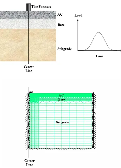
4.3 Axisymmetric Pavement Structure Modeling Subject to Cyclic Loadings 65
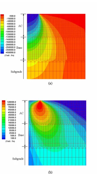
4.4 Stress Discontinuity: (a) Radial Stress; (b) Circumferential Stress 66
4.5 Stress Continuity: (a) Axial Stress; (b) Shear Stress 67
4.6 Chosen Locations for Checking the Normalized Error Norms 68
4.7 Convergence of the Normalized Error Norm in an AC Layer 69
4.8 Convergence of the Normalized Error Norm in a Base Layer 69
4.9 Convergence of the Normalized Error Norm in a Subgrade Layer 70
5.1 Uniaxial Monotonic Tension Lab Test Results: (a) Stress/Strain Behavior
and (b) Characteristic Damage Function (Chehab, 2002) 85
5.2 Axisymmetric FE Model: (a) Uniform Pressure; (b) Non-uniform Pressure 86
5.3 Asphalt Concrete Pavement Structure Simulated by the VECD-FEP++:
5.4 Thin AC Cases under Uniform 40 kN Load for: (a) MODULUS SS,
(b) MODULUS SW, (c) MODULUS WS, and (d) MODULUS WW 88
5.5 Medium AC Cases under Uniform 40 kN Load for: (a) MODULUS SS,
(b) MODULUS SW, (c) MODULUS WS, and (d) MODULUS WW 89
5.6 Thick I AC Cases under Uniform 40 kN Load for: (a) MODULUS SS,
(b) MODULUS SW, (c) MODULUS WS, and (d) MODULUS WW 90
5.7 Thick II AC Cases under Uniform 40 kN Load for: (a) MODULUS SS,
(b) MODULUS SW, (c) MODULUS WS, and (d) MODULUS WW 91
5.8 Thin AC Cases under Non-uniform 40 kN Load for: (a) MODULUS SS,
(b) MODULUS SW, (c) MODULUS WS, and (d) MODULUS WW 92
5.9 Medium AC Cases under Non-uniform 40 kN Load for: (a) MODULUS SS,
(b) MODULUS SW, (c) MODULUS WS, and (d) MODULUS WW 93
5.10 Thick I AC Cases under Non-uniform 40 kN Load for: (a) MODULUS SS,
(b) MODULUS SW, (c) MODULUS WS, and (d) MODULUS WW 94
5.11 Thick II AC Cases under Non-uniform 40 kN Load for: (a) MODULUS SS,
(b) MODULUS SW, (c) MODULUS WS, and (d) MODULUS WW 95
5.12 Thin AC Damage Contours under Uniform and Non-uniform 20 kN Load
for: (a) MODULUS SS, (b) MODULUS SW, (c) MODULUS WS, and
(d) MODULUS WW 96
5.13 Medium AC Damage Contours for Base/Subgrade Modulus Combinations: (1) Uniform Pressure and AC I Stiffness; (2) Uniform Pressure
and AC II Stiffness; (3) Non-uniform Pressure and AC I Stiffness;
CHAPTER 1
INTRODUCTION
Fatigue cracking is one of the major distresses affecting the performance of
asphalt pavements. Fatigue cracks can initiate at the bottom of the asphalt concrete layer
due to tensile stresses developed because of flexure and propagate to the pavement
surface under repeated load applications. Recent research also suggests that fatigue
cracks can also initiate at the pavement surface due to tensile stresses resulting from the
interaction between truck tires and the pavement surface. These fatigue cracks propagate
through the asphalt concrete layer under repetitive loading. The tensile stress-strain
behavior of the material appears to be the major factor of material characterization that
needs to be understood to address both bottom-up and top-down fatigue cracking (Daniel
and Kim 2002).
There has been a considerable amount of research in developing, verifying, and
calibrating fatigue performance models. Historically, much of the work in this area has
been empirical in nature. Most of these models relate asphalt mixture properties and
responses measured from a representative volume element (RVE) to the number of cycles
to failure. Due to their empirical nature, these models require a large amount of
laboratory testing to cover the wide range of conditions encountered in the field.
A more fundamental approach to the prediction of fatigue damage growth in
asphalt pavements is two-fold. First, material constitutive models need to be developed.
These models should be able to describe stress-strain behavior of layer materials in
Well-established theories in the discipline of material mechanics are available for this task.
The second step is to incorporate the material constitutive models into a structural model
that computes stresses and strains in pavement structures. This structural model accounts
for the effects of boundary conditions (such as layer thicknesses, pavement edges,
bedrock, etc.) for the pavement in question.
As discussed by Huang (1993), the classical approach to fatigue cracking
performance prediction employs the relationship between the allowable number of load
repetitions and the tensile strain at the bottom of the asphalt layer. However, Myers et al.
(2001) showed the traditional bottom-up crack of the cumulative damage concept fails to
predict the damage due to longitudinal surface cracking found in the field. They used the
linear elastic model for all the layers in pavement structures and incorporated fracture
mechanics into a finite element analysis to evaluate top-down cracking mechanisms. For
more realistic modeling however, the viscoelastic nature of asphalt concrete needs to be
accounted for in the analysis. Additionally, many researchers have found that the
nonlinear elastic behavior of base and subgrade materials is important in accurately
estimating stresses and strains in pavements.
The principal objective of this study is to study the fatigue cracking mechanisms
of asphalt pavements by evaluating stress and damage contours determined from a finite
element analysis that employs a viscoelastic continuum damage model for asphalt layer
and a stress-state dependent nonlinear elastic model for aggregate base and subgrade.
Effects of various pavement and load factors on the cracking mechanisms are also
to shed some light on identifying conditions that are more susceptible to either bottom-up
cracking or top-down cracking.
Chapter 2 describes the research effort made to implement the viscoelastic
continuum damage model into VECD-FEP++ on the foundation of FEP++ developed by
Guddati (2001). Methods of conversion among the linear viscoelastic functions and
numerical formulations for the implementation of the convolution integral are discussed.
Results from constant-crosshead-rate monotonic tests in tension at varying temperatures
and strain rates are used to verify the resulting finite element program. In Chapter 3, the
stress-state dependent nonlinear elastic model is included in the framework of
FEP++. The developed methodology was verified by comparing the results from
VECD-FEP++ with an analytical solution in a simple boundary condition and with the results
from laboratory resilient modulus tests of granular materials and fine-grained soils. In
Chapter 4, the finite element (FE) mesh discretization technique is treated in detail for the
analysis of multilayered pavement structures. Chapter 5 describes the investigation of the
fatigue failure modes by monitoring the stress and damage contours computed from
VECD-FEP++ with the viscoelastic continuum damage model and the nonlinear elastic
model. This chapter also presents findings from the parametric study in which the effects
of asphalt layer thickness, base/subgrade moduli, contact pressure distribution, and load
level are evaluated systematically. Finally, a summary of findings and recommendations
CHAPTER 2
MODELING OF ASPHALT LAYER IN PAVEMENT STRUCTURE
Top layer in a flexible pavement structure is made of asphalt concrete that is viscoelastic and undergoes damage under repeated loadings. In this chapter, the asphalt
layer is modeled using a viscoelastic continuum damage (VECD) model embedded into finite element (FE) discretization. This is performed using the following steps:
1) Obtaining the linear viscoelastic properties from experimental data (Section 2.1).
2) Incorporation of viscoelastic material properties into FE methods (Section 2.2).
3) Expansion of the material model to include damage and its implementation into FE
framework (Section 2.3).
2.1 LINEAR VISCOELASTIC MATERIAL MODELING
Linear viscoelastic material property of asphalt concrete is represented by a generalized Maxwell model, which can be viewed as a Prony series expansion of the relaxation modulus. The Prony series coefficients are estimated from the experimental
data using the following material modeling procedure:
1) Obtain complex moduli as a function of loading frequency using a frequency sweep
test and smoothening experimental data.
2) Convert the frequency domain data into time domain data (Prony series representation) with the positive sign control of the Prony series coefficients.
2.1.1 Techniques for Obtaining Material Properties
Frequency Sweep Test
The frequency sweep test (FST) is performed by applying a sinusoidal load to an
asphalt concrete specimen to obtain the linear viscoelastic material properties of asphalt mixtures. The loading amplitude is adjusted based on the material stiffness, temperature,
and frequency to keep the strain response within the linear viscoelastic range. Typically, a micro-strain level of 50 to 75 is targeted as the limit for the linear viscoelasticity. The loading is applied until steady-state response is achieved, at which point several cycles of
data are collected. After each frequency, a five-minute rest period is allowed for specimen recovery before the next loading block is applied. The frequencies are applied
from the fastest to the slowest ranging from 1 to 20 Hz.
From the FST, the complex modulus, E*, which includes the dynamic modulus
(|E*|) and the phase angle (φ), can be determined. The complex modulus can also be
viewed as a composition of storage (E′) and loss moduli (E″) as follows:
''
'
*
E
iE
E
=
+
(2.1)where i is the −1. The dynamic modulus is the amplitude of the complex modulus and is defined as:
2 2 ( '')
) ' ( | *
|E = E + E . (2.2)
The values of the storage and loss moduli, which are shown in Fig. 2.1, are related to the dynamic modulus and phase angle as follows:
φ
cos | * | ' E
Figure 2.1 Complex Modulus Schematic Diagram
As the material becomes more viscous, the phase angle increases and the loss
component of the complex modulus increases. Conversely, a decreasing phase angle indicates more elastic behavior and a larger contribution from the storage modulus. The
dynamic modulus at each frequency is calculated by dividing the steady state stress amplitude, σamp, by the strain amplitude, εamp:
amp amp E
ε σ
=
| *
| . (2.4)
The phase angle, φ, is associated with the time lag, ∆t, between the strain input and
stress response at the corresponding frequency, f:
t f∆ = π
φ 2 . (2.5)
As the testing temperature decreases or the loading rate increases, the dynamic modulus will increase and the phase angle will decrease indicating decreased history dependence or the viscoelasticity of the material.
Loss Modulus
,
E’
’
Storage Modulus, E’ |E*|
E*(E’, E’’)
Fitting Data to Log-Sigmoid Function
The storage modulus, E’(ω), can be obtained from Eq. (2.3) where ω represents a
reduced frequency at a given temperature. Fitting this data to a log-sigmoid function is
used to smoothen and average the oscillating data. The following equation, f(ω), is
defined as the log-sigmoid function:
[
]
+ +
+ =
) ( log exp
) (
10 6 5
4 3
2 1
ω ω
a a
a a
a a
f (2.6)
where a1,2, . . . , 6 are the coefficients determined by the iterative Levenberg-Marquardt algorithm (Fletcher, 1987), which minimizes the error in the approximation.
Figure 2.2 Fitting Experimental Data to Log-sigmoid Function 10
100 1000 10000 100000
0.00001 0.0001 0.001 0.01 0.1 1 10 100 1000 10000 100000 Reduced Frequency (rad)
S
to
rage Modulus
(k
Pa)
The Levenberg-Marquardt optimization is performed using the nonlinear-least-squares program in MATLAB. To obtain the best fit, the initial values of coefficients defined by Eq. (2.6) are iteratively changed until the log-sigmoid curve satisfactorily
represents the experimental storage data shown in Fig. 2.2. The smoothened storage moduli, fitted with the log-sigmoid function, are used for the following interconversion between frequency-domain modulus and time-domain (relaxation) modulus.
Frequency Domain Modulus to Time Domain (Relaxation) Modulus
The interconversion of linear viscoelastic material functions between frequency-domain and time-frequency-domain relaxation can be performed through either an approximate method or an exact method. Schapery and Park (1999) proposed the following
approximate analytical method, which is given by:
) / 1 ( | ) ( ' ' 1 )
(t E t
E ≅ ω ω=
λ (2.7)
where ω, t, E’(ω), and E(t) are reduced frequency, reduced time, storage modulus, and
relaxation modulus at a reference temperature respectively. The adjustment function, λ’,
is defined as follows:
) 2 / cos( ) 1 (
' π
λ =Γ −n n (2.8)
where Γ is a gamma function and n is the local log-log slope of the storage modulus given by:
ω ω
log ) ( ' log
d E d
n= . (2.9)
∑
=∞+ −
= M
m m m
t E
E t E
1
) / exp( )
( ρ (2.10)
where E∞, ρm, and Em are infinite relaxation modulus, relaxation time, and Prony
coefficients respectively. E∞ can be determined by E’(ω)|ω–>0+ using a very small
non-negative value of frequency. It is assumed that the collocation points of time (t) and ρm
are separated by decades (Schapery, 1961). Eq. (2.10) can then be viewed in the following matrix form:
N } { ]
[ 1 }
{
) / exp( )
(
C m
B M
m n m
A
n E t E
t E
− ∞ =
∑
= − ρ , n=1,…,N . (2.11)Note that the vector {C} is subjected to an additional constraint Em >0. This
constraint converts the parameter estimation problem into the following linear
programming problem:
MINIMIZE |[B]{C}-{A}| SUCH THAT {C}>0. (2.12) The above problem is solved by MATLAB.
Figure 2.3 Wiechert Model (or Generalized Maxwell Model)
..…
∞ E
1
E E3 EM−1 EM
1
η η2 η3 ηM−1 ηM
σ
An alternative to the above approximate method is an “exact” method outlined below. The interconversion between frequency-domain and time-domain material properties can be solved based on the following relations. As shown in Fig. 2.3, from a
given strain, ε, the stress in the left spring, σ∞, is:
ε
σ∞ =E∞ . (2.13)
The stress, σm, in each of the Maxwell components combining a spring with a dashpot is
governed by the differential equation:
m m m m dt d E dt d η σ σ
ε = 1 +
(2.14)
where ηm is the coefficient of viscosity, and Em is the relaxation modulus in the mth
term or Prony coefficient. Due to the linearity of the material components, the total stress on the Wiechert model is obtained by the following summation form:
∑
=∞+
= M
m 1 m
σ σ
σ . (2.15)
Fourier transformation converts the differential equation into the following
algebraic equation: ε ρ ω ρ ω σ + + =
∑
= ∞ Mm n m
m m n i E i E 1 1
, n=1,…,N (2.16)
where σ and ε are Fourier-transforms of stress and strain respectively, and the relaxation time of the mth Maxwell element is as follows:
m m
m ηE
ρ ≡ . (2.17)
∑
=∞+ +
= M
m n m
m m n i E i E E 1 1 * ρ ω ρ ω
, n=1,…,N. (2.18)
The storage modulus is obtained by taking the real part of the complex modulus:
∑
= ∞ + + = Mm n m
m m n
n E E
E
1 2 2 2 2 1 ) ( ' ρ ω ρ ω
ω , n=1,…,N. (2.19)
The parameters E∞, ρ∞, and Em are obtained by fitting the above expression with
the experimental storage modulus. E∞ can be found by E’(ω)|ω–>0+. Em can be obtained
based on matching the log-sigmoid function-fitted data with analytical expression in Eq.
(2.19) at discrete values of frequency ωn.
{D}=[E]{F} (2.20)
where the column vectors, {F} and {D}, are Em and E’(ωn)-E∞ respectively; the matrix,
[E], is as follows:
∑
= +
= M
m n m
m n m
n
E
1 2 2 2 2 , 1 ρ ω ρ ω
, n=1,…,N. (2.21)
However, the solution of Eq. (2.20) does not guarantee the positive coefficients of Em. Obtaining the positive coefficients of Em can be done by introducing the constraints that
force them to be non-negative and minimizing the error of the fit. The problem is then the linear programming problem, which is solved by MATLAB.
MINIMIZE |[E]{F}-{D}| SUCH THAT {F}>0. (2.22)
2.1.2 Evaluation of Material Property Estimation Techniques
Table 2.1 Five Sets Chosen in This Study
Combination Dynamic Modulus Phase Angle Conversion Method
1 Raw Raw Exact
2 Average Adjusted Exact
3 Average Average Exact
4 Average Adjusted Approximate
5 Average Average Approximate
The experimental dynamic moduli can be chosen by using them as they are or by averaging them. The phase angles are chosen as the raw phase angles, averaged phase
angles or they can be adjusted to be decreasing function of the frequency (see Fig. 2.4). Two asphalt concrete specimens were subject to eight FSTs at five different temperatures (e.g., targeted –10°, 5°, 15°, 25°, and 35°C). Using time-temperature
superposition principle, all the data are translated to a reference temperature of 5°C for
the further comparison using raw data and processed data. The Prony-series representation curves determined from the suggested combinations are shown in Fig. 2.5. Since all the combinations perform equally well, Combination 3 is chosen based on its
Figure 2.4 Adjusted Phase Angle at Temperature 5°C
Figure 2.5 Relaxation Modulus Generated by Prony-Series Representation at 5°C
0 5 10 15 20 25 30 35 40 45 50
0.000001 0.00001 0.0001 0.001 0.01 0.1 1 10 100 1000 10000 Reduced Frequency (Hz)
Ph
as
e A
ngl
e (d
egree)
FST 1 FST 2 FST 3 FST 4 FST 5 FST 6 FST 7 FST 8 Adjusted
1.E+00 1.E+01 1.E+02 1.E+03 1.E+04 1.E+05
1.E-07 1.E-05 1.E-03 1.E-01 1.E+01 1.E+03 1.E+05 1.E+07 1.E+09 1.E+11 1.E+13 Reduced Time (sec)
Re
la
xa
tion
M
odu
lu
s
(M
P
a)
2.2 NUMERICAL INTEGRATION OF LINEAR VISCOELASTICITY
To solve the initial-boundary value problem involving linear viscoelasticity, the constitutive equation between stress and strain expressed in the convolution integral form
of the relaxation modulus needs to be numerically integrated. Three techniques of numerical integration are evaluated here: composite trapezoidal integration, parabolic algorithm, and internal state variable approach.
The trapezoidal rule of convolution integral is employed based on the simple numerical procedure given by Linz (1985). The parabolic algorithm is implementing
forward Euler, Crank-Nicolson, and backward Euler methods for the time-discretization as discussed by Hughes (2000). The numerical integral formulation of the internal state variable method for the constitutive modeling of viscoelastic materials is implemented
based on the approach presented in Simo and Hughes (1998).
2.2.1 Numerical Integration Schemes
Composite Trapezoidal Rule
The relaxation modulus for a viscoelastic material is determined by stress
responses from a strain history input; the following constitutive relation can be defined using the relaxation modulus in the form of the convolution integral:
τ τ
τ ε τ
σ d
d d t E t
t
∫
∞ −−
= ( ) ( ) )
( (2.23)
where )σ(t is the stress, E(t) is the relaxation modulus, and ε(t) is the strain.
The constitutive equation for the considered viscoelastic materials in this work is derived using the Prony series of the relaxation modulus in Eq. (2.10). The following
∫
− +=g t tk t d
t 0 ) ( ) ( ) ( ) ( τ ε τ τ
ε (2.24)
where, ) 0 ( / ) ( )
(t t E
g =σ ,
∑
= − − = − = − M m m m t E E t E d d E t k 1 )) ( exp( ) 0 ( 1 ) ( ) 0 ( 1 ) ( τ ρ τ ττ , and
∑
= ∞ + = M m m E E E 1 ) 0 ( .The approximate solution εh(t) of the Volterra equation can be computed by
replacing the integral on the right hand side of Eq. (2.24) by a numerical trapezoidal rule
using values of the integrand at ti, i=0,1,...,n including the known equation of σ(t).
Since ε(t0=0)= g(t0=0), the linear numerical solution of strain εh(tn) can be found in the
following step-by-step scheme:
) ( )
( n n
h t =g t
ε − + − + − ∆ +
∑
− = 1 1 00 2 ( ) ( )
1 ) ( ) ( ) ( ) ( 2 1 n
i n i i n n n
n t t k t t t k t t t
t k
t ε ε ε ; (2.25)
− + − ∆ + = −∆
∑
− = 1 1 00) ( ) ( ) ( )
( 2 1 ) ( ) ( ) 0 ( 2 1 n i i i n n n n
h t g t t k t t t k t t t
k
t ε ε ε
. (2.26)
In Box (2.1) the algorithm for the numerical trapezoidal rule is outlined. To perform semi-discrete time error analysis, the following theorem is applied to obtain the order of
Box 2.1 Numerical Trapezoidal Algorithm
Theorem 2.1. Let K(t,τ,ε(τ)) be second-order differentiable with respect to time with
n t t= n/
∆ and ti =i∆tfor each i =0,1,...,n. The composite trapezoidal rule for nth
subinterval is:
∫
t K t d0 )) ( , , ( τ ε τ τ = + + ∆
∑
− = 1 1 00 ( , , ( ))
2 1 )) ( , , ( )) ( , , ( 2 1 n i n n n i i n
n t t K t t t K t t t
t K
t ε ε ε
( , , ( )) 12 2 s s n
n t K t t t
t ∆ ε
−
for some ts ∈(0,tn), where double overdot denotes double time derivative.
Proof.
If Pn is the Lagrange interpolating polynomial,
∑
= = n i i i i nn t K t t t L t
P 0 ) ( )) ( , , ( )) ( , , ( τ ε τ ε
where
∏
≠ = − − = n i j
j i j
j i t t t t t L
0 ( )
) ( )
( .
Now, Pn and its truncation error term are integrated over [0, tn] to obtain
With known ε(ti, i=1,..,n−1), ∆t, and g(tn) at nth step
Compute (0) 2 1
0 k
t
A = −∆ and
− + − ∆ =
∑
− = 1 1 00) ( ) ( ) ( )
( 2 1 n i i i n n
n t k t t t k t t t
A ε ε
Obtain 0 ) ( ) ( A A t g
t n n
∫∏
∫
∫∑
= + = + − += t n
i s s n n i n
t t n
i
i i i
n K t t t dt
n t t dt t L t t t K d t K 0 0 ) 1 (
0 0 0
)) ( , , ( )! 1 ( ) ( ) ( )) ( , , ( )) ( , , ( τ ε τ τ ε ε
∑
∫∏
= = + − + + = n i t n i s s n n i n i i ni t t K t t t dt
n t t t K a
0 0 0
) 1 ( )) ( , , ( ) ( )! 1 ( 1 )) ( , , ( ε ε
where ai =
∫
t Li t dt0
)
( .
Let’s consider the example of ( , , ( ))
) ( ) ( )) ( , , ( ) ( ) ( 1 1 1 0 1 0 0 0 1 1 0 1
1 K t t t
t t t t t t t K t t t t
P ε ε
− − + − − = . Therefore,
∫
1 = − + − −0 )) ( , , ( 12 ) ( ))] ( , , ( )) ( , , ( [ 2 ) ( )) ( , , ( 1 3 0 1 1 1 1 0 0 1 0 1 t t s s i i
n K t t t
t t t t t K t t t K t t dt t t t
K ε ε ε ε .
This integration between t0 and t1 can be extended to multi-time discrete trapezoidal rule
such as ti,i=0,1,...,n by induction.
The error estimate related to time discretization can be easily obtained based on
Theorem 2.1. Subtracting Eq. (2.25) from Eq. (2.24) gives:
2
) ( )
(t −εh t ≤C∆t
ε (2.27)
where C is a positive constant independent of ε.
Parabolic Algorithm
The parabolic equation can be constructed based on using Eqs. (2.13) to (2.15). First, Eq. (2.15) is differentiated with respect to time and then the differentiated Eq.
[ ] { } [ ]{ } { } F d M Q M d M P M t dt d t t dt d E E E − = + − − − − − ∞ 0 . . 0 ) ( . . ) ( / 1 0 0 0 0 0 . 0 0 . 0 0 . 0 . 0 0 0 / 1 . 0 . . . 0 . . ) ( / 1 0 0 0 1 0 . 0 0 . 0 0 . 0 . 0 0 0 / 1 1 1 . . 1 1 1 1 1 σ σ σ ε η η σ σ ε or
[ ]
P{
d}
+[ ]
Q{ } { }
d = F (2.28)where overdot denotes time derivative.
The initial value problem consists of finding a function
{ } { }
d = d(t) , whichsatisfies Eq. (2.28) and the initial condition
{
d(t0 =0)} { }
= d0 . The initial condition canbe determined from Eq. (2.24) at t0, which is ε(t0)=g(t0), and the values σm (m=1,…,M)
being all zeros at t0. For the discretization in time, the classical methods such as forward
Euler, Crank-Nicolson, and backward Euler can be considered. These methods can be considered as special cases of the following general scheme (Hughes, 2000):
[ ]
P{ }
v n+1+[ ]
Q{ }
d n+1 ={ }
F n+1 (2.29)
{ }
d n+1 ={ }
d n +∆t{ }
v n+α (2.30)
{ }
v n+α =(1−α){ }
v n +α{ }
v n+1 (2.31)where
{ }
d n and{ }
v n are the approximate solutions to{
d(tn)}
and{ }
d(tn) respectively;t
∆ is a constant time increment;
{ }
F n+1 ={
F(tn+1)}
. Forward Euler, Crank-Nicolson, andbackward Euler methods can be obtained by choosing the value α = 0, ½, or 1
Box 2.2 Numerical Parabolic Algorithm
Before the order of accuracy in parabolic algorithm is determined, the required property is the stability, which depends on the choice of α value. To find the appropriate
indication of the stability, the homogeneous equation of Eq. (2.28) can be changed into
modal representation:
{ }
d +λ{ }
d =0 (2.32)where λ is eigenvalue of
[ ]
Q with respect to[ ]
P . The above equation, whendiscretized in time, results in a relation between dn+1 and dn as follows:
n
n d
t t d
) 1
(
) 1 ( 1 (
1 α λ
λ α
∆ +
∆ − − =
+ (2.33)
With the known
{ }
d and n{ }
v nCompute the predictor value of dn+1:
n n
n d t v
dˆ} { } (1 ) { } { +1 = + −α ∆
Using Eqs. (2.38) and (2.39), obtain the corrector value:
1 1
1 {ˆ} { }
}
{d n+ = d n+ +α∆t v n+
To obtain vn+1, the above equation substituted into Eq. (2.37)
) } ˆ ]{ [ } ({ ]) [ ] ([ }
{ 1 1 1
1 − + +
+ = + ∆ n − n
n P t Q F Q d
v α
Update {d}n+1
which implies that dn+1 ≤ Am dn . The amplification factor ) 1 ( ) ) 1 ( 1 ( λ α λ α t t Am ∆ + ∆ − − =
should be less than one for stability of the time-integration. It can be seen that
Crank-Nicolson and backward Euler methods are unconditionally stable; however, the forward Euler method has the following stability condition:
λ
2 <
∆t . (2.34)
Considering an example with E(t)=1+exp(−t), two eigenvalues, λ1 =0 and
=
2
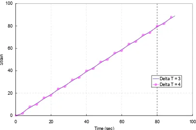
λ 0.5, can be obtained. For stability, ∆t should be less than 4. Figs. 2.6 and 2.9 show
the results for various values of ∆t(e.g., ∆t =3, 4 and 5). It can be clearly seen that
when the time step size is larger than the stability limit (∆ =t 4), the solution is unstable.
The order of accuracy in time discretization is evaluated based on Taylor series
analysis of the truncation error. We expand the function values of
{ }
d in a Taylor seriesabout t as follows:
{ }
{
} { }
{ }
{ }
{ }
( ) ( ) 6 1 ) ( 2 1 ) ( ) ( )( 2 3 4
1 d t t d t t d t t d t t d t O t
d n+ = +∆ = +∆ + ∆ + ∆ + ∆ ; (2.35)
{ }
{
} { }
{ }
{ }
{ }
( ) ( ) 6 1 ) ( 2 1 ) ( ) ( )( 2 3 4
1 d t t d t t d t t d t t d t O t
d n− = −∆ = −∆ + ∆ − ∆ + ∆ , (2.36)
which results in the following relations:
{ }
{ }
{ }
{ }
{ }
) ( 6 1 21 2 3
1 d t d t d O t
t d d n n n n
n − = ∆ + ∆ + ∆
∆ −
+ ; (2.37)
{ } { }
{ }
{ }
{ }
( )6 1 2
1 2 3
1 d t d t d O t
t d d n n n n
n − =− ∆ + ∆ + ∆
∆
− −
Figure 2.6 Instability at ∆t=4
Figure 2.7 Instability at ∆t=5
0 20 40 60 80 100
0 20 40 60 80 100
Time (sec)
St
rain
Delta T = 3 Delta T = 4
-1500 -1000 -500 0 500 1000 1500 2000
0 20 40 60 80 100
Time (sec)
St
ra
in
Eq. (2.37) indicates the first order of accuracy in the forward Euler method. Similar argument can also be applied to backward Euler method. On the other hand, Crank-Nicolson method results in second order accuracy, which is based on the following
observation:
{ }
1{ }
{ }
2{ }
31 1
2 2
1
( ) 6
n n
n n
d d
d t d O t
t +
+ +
−
− = ∆ + ∆
∆ . (2.39)
Internal State Variable Approach
The internal state variable approach is based on the time discrete problem of the
left hand side of Eq. (2.14), which is (εn+1 −εn)/∆t, with the known initial state variable
σm = σmn at t=tn. The ∆t can be chosen to be constant in this study. The solution of the
discrete Eq. (2.14) is an exponential form as follows:
[
]
exp ( ) /
m a b t tn m
σ = + − − ρ (2.40)
where a and b are constants. Based on the assumption of linearity between εn+1and εn,
substituting Eq. (2.40) into Eq. (2.14) is carried out to obtain the constant a as follows:
[
]
{
[
]
}
11 1
( ) exp ( ) / exp ( ) /
n n
n m n m
m m m
b
t t a b t t
E t
ε ε
ρ ρ
ρ η
+ −
− − − + + − − =
∆ . (2.41)
Because ηm equals to Emρm, the above exponential terms are canceled out and then, the
constant a is found in the following form:
t a
n n
m ∆
−
=η ε +1 ε . (2.42)
The initial state variable, which σm=σmn at t=tn, is substituted into Eq. (2.40) for
a
b n
m−
=σ . (2.43)
According to the constitutive equation of Eq. (2.15), the determined constants, a and b,
are used to obtain the following state variable expression at t t= n+1:
) ( ) / exp( 1 ( ) / exp( 1
1 n n
Mod m m n m m n m m res m t t
t ρ σ η ρ ε ε
σ σ − ⋅ ∆ − − ∆ + ∆ − = + +
; (2.44)
and therefore,
∑
∑
= + = + ∞ + = + + − M m n n m M m res m nn E Mod
t
1
1 1
1
1) ( )
( ε σ ε ε
σ . (2.45)
The implementation of internal state variable algorithm is illustrated in the following Box 2.3.
Box 2.3 Numerical Internal State Variable Algorithm
For the error estimate of the state variable approach, the following second-order
accuracy is determined based on the linearity between εn+1and εn:
With the known σ(tn+1), εn, and n m
σ at t=tn
Obtain
∑
= = M m m Mod Mod 1
and
∑
= = M m res m res 1 σ σ Compute ) ( ) ( 1 1 Mod E Mod
t res n
n n + ⋅ + − = ∞ + + σ σ ε ε
Update 1 ( n 1 n)
m res
m n
m σ Mod ε ε
σ + = + + −
2 2
/ 1
1 C t
t n
n
n − ≤ ∆
∆ − + + ε ε ε (2.46)
where C is a positive constant independent of ε.
2.2.2 Numerical Tests for Time Integration
Two examples (see Table 2.2) are used to evaluate the performance of the three
different numerical integration algorithms.
Table 2.2 Relaxation Modulus and Creep Compliance Used in Numerical Examples
Example Relaxation Modulus Creep Compliance
I E(t)=1+exp(−t) 1−0.5⋅exp(−t/2)
II E(t)=1+exp(−t)+2⋅exp(−t/2)
)] 2 / exp( ) 2 2 3 ( 2 2 3 [ ] ) 2 2 ( 25 . 0 exp[ 125 . 0 1 t t ⋅ + + − ⋅ + − ⋅ −
In order to get the exact solutions in terms of calculating strain components, creep compliance, )D(t , is required to construct the following constitutive relationship between
strain and stress:
τ τ σ τ ε d d d t D t t
∫
− = 0 ) ( )( . (2.47)
Therefore, an elastic-viscoelastic correspondence principle is adopted. The correspondence principle reveals that the static elastic solutions can be converted to
E, by creep compliance, D, can be expressed in terms of the Carson or Laplace transformation in the following form:
1 ~ ~ =
D
E or 12 s D
E = (2.48)
where and ¯ denote the Carson and Laplace transforms respectively, and s represents Laplace parameter. Using Eq. (2.48), the creep compliances corresponding to relaxation
moduli can be obtained from solving the Laplace-transformation and -inversion problems. Table 2.2 shows the calculated creep compliances related to relaxation moduli
used in this study.
The example constitutive relations are numerically integrated using the composite trapezoidal integration, parabolic algorithm, and internal state variable approach. The time history of stress in both examples is chosen as t⋅H(t) where H(t) is a Heaviside step
function. The time step sizes are chosen as 0.1, 0.05, 0.025, 0.0125, and 0.00625. The resultant strains are compared with the exact strains and the errors are examined in Figs.
2.8 and 2.9. Fig. 2.8 shows that the forward and backward Euler approaches provide first-order accuracy; other methods have second-order accuracy. In particular, both
Figure 2.8 The Maximum of Absolute Errors in the Numerical Methods of Example I
Figure 2.9 The Maximum of Absolute Errors in the Numerical Methods of Example II
0.0000001 0.000001 0.00001 0.0001 0.001 0.01 0.1
0.001 0.01 0.1 1
Log(Incremental Time)
L
og(Max
im
u
m
of
Abs
olut
e Error
)
Forward Euler Backward Euler Crank-Nicolson Internal State Variable Trapezoidal Rule
0.00000001 0.0000001 0.000001 0.00001 0.0001 0.001 0.01 0.1 1
0.001 0.01 0.1 1
Log(Incremental Time)
L
og(Max
im
u
m
of
Abs
olut
e Error
)
2.3 VISCOELASTIC CONTINUUM DAMAGE MODEL
2.3.1 Material Modeling
Asphalt concrete is modeled as a thermorheologically simple material undergoing
damage that is characterized with the help of the work potential theory. In this section, the work potential theory for viscoelastic damage mechanics is discussed in the
framework of elastic damage mechanics coupled with the viscoelastic correspondence principle. The rest of the section describes: (a) the time-temperature superposition arising from thermorheological simplicity; (b) the work potential theory for damage in elastic
solids; (c) the viscoelastic correspondence principle facilitating the link between the elastic damage theory and viscoelastic damage theory; and finally, (d) the complete
viscoelastic damage theory.
All these theories are discussed using experimental results presented in Fig. 2.10, which contains the stress-strain relationships obtained using constant crosshead
displacement rate tests.
Time-Temperature Superposition
The time temperature superposition states that the stress-strain behavior at a particular temperature at a given strain rate is identical to the stress-strain behavior at
another temperature at a modified strain rate. This modified strain rate is obtained by simply scaling the time with a function of the temperature (aT) using the following law:
R T t
a
where tR is the (reduced) time at the reference temperature (chosen to be 5ºC for this study), t is the time at the given temperature, and aT is the time-temperature shift factor. For the given data, the shift factor is observed to be:
aT = 0.0002( .) 0.1308( .) 0.6582
2
10− Temp − Temp + .
Note that Fig. 2.10 contains experimental results at several temperatures, but the
rates given in the figure are reduced rates at the reference temperature of 5ºC (see Table 2.3 for details). The magnified stress-strain curves in Fig. 2.11 clearly indicate the
rate-dependent behavior of asphalt concrete – the material is generally stiffer and stronger at faster rates. For the remainder of this dissertation, all the experimental data will be viewed in the context of the reduced strain rates at the reference temperature.
Table 2.3 Reduced Strain Rate and Material Parameters of the Damage Function
Strain Rate Reduced Strain Rate at a Reference Temp. 5ºC Initial Pseudo Stiffness (I) C(S) 0.00003/sec at 5ºC 0.00003/sec 0.81 0.81·Ĉ(S) 0.000056/sec at 5ºC 0.000056/sec 0.80 0.80·Ĉ(S) 0.000012/sec at 5ºC 0.000012/sec 1.02 1.02·Ĉ(S) 0.0135/sec at 25ºC 0.000026/sec 1.10 1.10·Ĉ(S) 0.0045/sec at 25ºC 0.0000086/sec 1.08 1.08·Ĉ(S) 0.0005/sec at 25ºC 0.000001/sec 1.15 1.15·Ĉ(S)
Figure 2.10 Stress/Strain Curves for Reduced Strain Rates in Tension
0 500 1000 1500 2000 2500 3000
0 0.0005 0.001 0.0015 0.002 0.0025 0.003 0.0035 0.004 0.0045
Strain
S
tress (kP
a)
0.000001/sec 0.0000086/sec
0.000012/sec 0.000026/sec
0.00003/sec 0.000056/sec
0 400 800 1200
0 0.00005 0.0001 0.00015 0.0002
Strain
S
tre
ss (kP
a
)
Elastic Damage Models
Schapery (1990, 1991) proposed a simple model for viscoelastic composites with growing damage that is based on replacing the physical displacements by quantities
called pseudodisplacements. An elastic material’s thermodynamic state is a function of independent generalized displacements, qj (j=1,2…J), and internal state variables, Sm
(m=1,2…M), where the inelastic behavior is captured from changes in Sm. Generalized
forces, Qj, are defined for each virtual displacement, δq, and virtual energy, δW, in the
following form:
j
j W q
Q =∂ /∂ . (2.50)
In isothermal conditions, the virtual energy, W, is the Helmholz free energy. Therefore,
W can be viewed as the strain energy depending on the strain tensor, εij, and internal state
variables, Sm. In a standard physical setting of stress and strain, Eq. (2.50) becomes
ij ij
W ε σ
∂ ∂
= (i; j =1,2,3) (2.51)
where σij are the stress components of the constitutive equation in the form of tensor
notation.
The internal state variables are chosen to account for changes in the structure such
as micro- or macrocracking based on the following damage evolution laws:
m S
m S
W S
W ∂ ∂ = ∂
∂
where WS=WS(Sm) is the dissipated energy due to damage growth. The left side of Eq.
(2.52) is the available thermodynamic force for damage growth while the right side is the required force.
The above work potential theory is used as a guide to develop a three-dimensional constitutive relationship from the axisymmetric damage model. As suggested by
Schapery, the elastic strain energy density for a locally transversely isotropic composite material can be written in the following form:
[
2 ( ) ( )]
2
1 2 2
12 66 2 23 2 13 44 12 2 22 2
11eV A ed A edeV A A eS
A
W = + + + γ +γ + γ + (2.53)
where x3 is the axis of material symmetry and
23 23 13 13 12 12 11 22 33 33 22 11 2 2 2 3 / ε γ ε γ ε γ ε ε ε ε ε ε = = = − = − = + +
= d V S
V e e e
e
(2.54)
and the five coefficients (e.g., A11, A22, A12, A44, and A66) are the elastic moduli depending
on the state of damage. When a uniaxial stress state is taken into account with a
maximum strain direction to the axis of x3 (e.g., ε11 = ε22, eS = 0, γ12 = 0, γ13 = 0, and γ23
= 0), the strain energy density Eq. (2.53) can be reduced to W’ independent of A44, in the
form: ) 2 ( 2 1 ' 2 66 12 2 22 2
11eV A ed A edeV A eS
A
W = + + + . (2.55)
The derivative of Eq. (2.55) with respect to the principal strains (e.g., ε’11, ε’22, and ε’33)
. ) 3 2 ( ) 3 2 ( ' ) 3 1 ( ) 3 1 ( ' ) 3 1 ( ) 3 1 ( ' 22 12 12 11 33 66 22 12 12 11 22 66 22 12 12 11 11 d V S d V S d V e A A e A A e A e A A e A A e A e A A e A A + + + = + − + − = − − + − = σ σ σ (2.56)
The relationship between the strains, εjk (j, k = 1, 2, 3) in the reference coordinate system,
and the principle strains, ε’ii (i = 1, 2, 3), is given by the general second order tensor
transformation below:
jk ik ij
ii ε
ε' =Ω Ω (2.57)
where the above transformation matrix Ωij is cosine(x’i, xj), which is the direction cosine
of the axes between x’i and xj. A similar transformation law applies for stresses:
ii T ij T ik
jk σ'
σ =Ω Ω . (2.58)
where •T denotes the transpose of a matrix and σ’
ii is a diagonal tensor containing the
principal stresses.
According to Schapery (1991) and Ha et al. (1998), the five coefficients, A11 to
A66, in Eq. (2.53), can be determined in terms of a damage function, C(S), Poisson’s ratio
υ, and Young’s modulus E:
Viscoelastic Correspondence Principle
Correspondence principles in linear viscoelasticity theory usually refer to elastic-viscoelastic relationships involving Laplace or Fourier transformed stresses and strains.
Instead, Schapery (1984) constructed a stress-strain constitutive equation for viscoelastic materials represented by an elastic-like relationship through the use of so-called
pseudovariables. The correspondence principles developed by Schapery for time-dependent, quasi-static solutions to nonlinear viscoelastic boundary value problems can be used to enable a viscoelastic solution to be easily constructed from the elastic solution
described in the above section. For linear viscoelastic materials, the stress-pseudostrain relationships take a form similar to elastic stress-strain relationships:
R kl R ijkl
ij C ε
σ = (2.60)
where
) ( ik jl il jk kl
ij R
ijkl
C =λδ δ +µ δ δ +δ δ , and
τ τ ε τ
ε E t d
E
t
kl
R R
kl
∫
∂∂ − = 0 ) ( 1
. (2.61)
CR
ijkl is the material constant, εklR is the pseudostrain tensor, ER is the reference modulus,
E(t) is the relaxation modulus, and λ and µ are Lamé constants in the following form:
. ) 1 ( 2 , ) 2 1 )( 1 ( υ υ µ υ υ λ + = − +
= ER ER (2.62)
Furthermore, υ is a constant Poisson’s ratio, and δij is the Kronecker delta:
≠ = = = j i j i ij ; 0 ; 1
Note that all the hereditary effects of the viscoelastic material are accounted for through the convolution integral in Eq. (2.61).
Viscoelastic Damage Models
Schapery further extended his elastic damage theory to viscoelastic materials with
the help of the correspondence principle (Schapery, 1984). To include the viscoelastic effects of microcracking, he proposed the following rate-type damage evolution law:
m
m R
m
S W S
α
∂ ∂ − =
(2.64)
where the overdot represents the derivative with respect to time, WR=WR(εijR, Sm) is the
pseudostrain energy density function, αm is a material-dependent constant, and m is not
summation. The available thermodynamic force, -∂WR/∂S
m, is similar to a crack growth
equation presented by Park el al. (1996). The form of the evolution law was adequate for
describing the multiaxial behavior of particulate composites with growing damage (Park and Schapery, 1997). In this study, this approach is applied to asphalt concrete materials.
In order to determine the damage model parameter of the rate-type damage
evolution, the stress responses at given strain rates and temperatures were measured, as shown in Fig. 2.14, under constant crosshead strain rate tests conducted on the cylindrical
specimens (Ghehab, 2002). Furthermore, LVDTs were mounted on the specimen surface to measure displacements with respect to time, and the displacement was converted into the effective strain applied to the specimen. However, the lab results obtained from
closed-loop servo-hydraulic MTS testing machine and the effective strains measured from the LVDT. In an attempt to ensure consistency in applying the viscoelastic theory with growing damage, the realistic strains from the LVDT were used for the analysis.
The experimental stress-strain constitutive relationship obtained from the above uniaxial tests was incorporated into the one-dimensional pseudostrain energy density
function of the material in the following form:
2
) )( ( 2
1 R
R C S
W = ε (2.65)
where the damage function, C(S) , depends on a single damage parameter, S. Then, the stress of Eq. (2.51) can be obtained based on Schapery’s correspondence principle, as
follows:
R R
R
S C
W ε
ε
σ = ( )
∂ ∂
≡ or C S R
ε σ
= )
( . (2.66)
Therefore, the damage function, C(S), can be determined using the experimental stress, σ,
and the pseudostrain, εR .
The pseudostrain is to be calculated using Eq. (2.61). Due to the expensive nature of the convolution integral, several authors have proposed efficient integration techniques (Taylor et al., 1970, Zocher et al., 1997, Kaliske et al., 1997, Poon et al., 1998, and Simo
et al., 1998), based on the following Prony series approximation of the relaxation modulus:
∑
=− ∞ +
= M
m
t
me m
E E
t E
1 /
)
where E¶, Em, and ρm are all constants. Using the above expression, it is shown that the
convolution in Eq. (2.61) can be replaced by the following recursive computation
(Hinterhoelzl, 2000): − =
∑
= + + + M m n m kl m n kl R n Rkl E E
E 1 1 , 1 0 1
, 1 ε ε
ε
with
∑
= ∞ + = M m m E E E 1
0 , and
(
)
[
n m]
m n t m n n n kl n kl n m kl t n kl n m
kl t e
t
e ρ ε ε ε ρ ρ
ε ε / 1 1 1 , / 1
, +1 ( ) 1 −∆ +1
+ + + ∆ − + ∆ − − ∆ ∆ + − +
= . (2.68)
In the above, the pseudostrain is split into M component pseudostrains based on the Prony series expansion of Eq. (2.67).
For uniaxial loading conditions, a single damage variable (S) is used along with the associated power, α . The value of α is obtained using the experimental data and by
the following incremental relationship obtained by combining Eqs. (2.64) and (2.65):
) 1 /( 1 2 ) ( 2
1 ε α +α
∆ − ∆ =
∆S C R t then,
) 1 /( 1 1 ) 1 /( 1 2
1 )( ) ( )
( 2
1 ε α α +α
− + = − − −
≅
∑
N n nn
R n n
n C t t
C
S . (2.69)
Using optimization search techniques and the data from the first two cases in Table 2.3, the value of α is found to be equal to 2.5. Furthermore, a relationship is constructed
Fig. 2.12). From Figs. 2.11 and 2.12, it can be observed that the stiffness scale factor, C(S), can be fit into the normalized functional form Ĉ(S) = exp(–0.00228·S0.506).
The three-dimensional continuum damage viscoelastic model is similarly obtained
by simply using the correspondence principle in the framework of three-dimensional elastic damage mechanics. Using this idea, the pseudostrain energy density function is
defined as:
( )
( )
[
( ) ( )
]
{
223 2 13 44 12
2 22 2
11 2
2
1 R R R
V R d R
d R
V
R A e A e A e e A
W = + + + γ + γ
( ) ( )
[
2 2]
}
12 66
R S
R e
A +
Figure 2.12 Normalized Damage Function/Parameter Curves for Two Fast-Reduced Strain Rates
Figure 2.13 Stress vs. Pseudostrain Plot to Obtain Initial Pseudostiffness
0 0.2 0.4 0.6 0.8
0 100000 200000 300000 400000 500000
Damage Parameter, S
N
ormaliz
ed D
amage Func
tion,
Ĉ
(S
)
0.00003/sec 0.000056/sec Fitted Function
0 100 200 300 400 500 600 700
0 100 200 300 400 500 600 700
Pseudo Strain
S
tress (kPa)
where . 2 2 2 3 / 23 23 13 13 12 12 11 22 33 33 22 11 R R R R R R R R R S R V R R d R R R R
V e e e
e ε γ ε γ ε γ ε ε ε ε ε ε = = = − = − = + + = (2.71)
In terms of principal pseudostrains,
( )
( )
( )
[
2]
66 12 2 22 2 11 2 2 1 ' R S R V R d R d R V
R A e A e A e e A e
W = + + + , (2.72)
that results in the following constitutive relationships between stress and pseudostrain:
. ) 3 2 ( ) 3 2 ( ' ) 3 1 ( ) 3 1 ( ' ) 3 1 ( ) 3 1 ( ' 22 12 12 11 33 66 22 12 12 11 22 66 22 12 12 11 11 R d R V R S R d R V R S R d R V e A A e A A e A e A A e A A e A e A A e A A + + + = + − + − = − − + − = σ σ σ (2.73)
2.3.3 Finite Element Implementation
Due to the nonlinear nature of damage, Newton-type iterative methods are needed
to solve the equilibrium equations. The tangent stiffness matrix needed in the solution procedure is obtained using the tangent modulus relating the infinitesimal increase in the stress to the infinitesimal increase in the strain. For damaged viscoelastic solids, the
tangent modulus is obtained using the following chain rule resulting from the ideas of the correspondence principle: kl R pq R pq ij kl ij ijkl C ε ε ε σ ε σ ∂ ∂ ⋅ ∂ ∂ = ∂ ∂ = (2.74)
For linear Viscoelasticity, the terms in the right side of the above equation are given by:
R ijpq R
pq ij =C
∂ ∂
ε σ