Comparative Analysis of Protein Datasets
using Firefly Optimization with Rough Set
Based Attribute Reduction (FFO_RSAR)
A. Revathi 1, Dr. P. Sumathi 2
Assistant Professor, Department of Computer Science, New Prince Shri Bhavani Arts and Science College,
Medavakkam, Chennai, Tamil Nadu, India1
Assistant Professor, PG & Research Department of Computer Science, Government Arts College,
Coimbatore, Tamil Nadu, India2
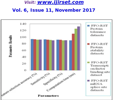
ABSTRACT: Data mining is the computing process of discovering patterns in large data sets involving methods at the intersection of machine learning, statistics, and database systems. Irrelevant, noisy and high dimensional data contain large number of features, which degrades the performance of data mining and machine learning tasks. One of the methods used to reduce the dimensionality of data is feature selection. Feature selection method selects a subset of features that represents original features in problem area with high accuracy. Various methods have been proposed to find these subsets. These methods either time consuming to find subset or support with optimality [1]. This paper presents a new feature selection approach that combines Firefly Optimization algorithm (FFO) with RoughSetTheory. The algorithm suggests that the attraction system of fireflies shows the feature selection procedure. The experimental results show the comparative analysis of various measures such as accuracy, specificity, and sensitivity and computation time with different protein data sets namely Protein tolerance datasets, Protein stability datasets, mRNA splice site datasets and Transcription factor binding site dataset
KEYWORDS: Feature Selection, Rough Set, Firefly Algorithm
I. INTRODUCTION
problem to be optimized. The proposed algorithm (FFO_RSAR) is an effort that combines FFO algorithm together with RST to ensure the data dependency in less time at the cost of the degree of optimality.
II. METHODOLOGY
A. Particle Swarm Based Reduct (PSO-RSAR)
The PSO algorithm[3] works by iterations in the search space. During each iteration, candidate solution is evaluated by the objective function which is being optimized, determining the fitness of that solution i.e. it determines how fit the solution is. From the fitness of that solution, find the maximum or minimum objective function. Initially, the PSO algorithm chooses candidate solution which is a set of possible values within the search space and uses the objective function to evaluate its candidate solutions, and brings about the resultant fitness values. Each particle maintains its position that composed of the candidate solution, its evaluated fitness, and its velocity. In addition to that, it finds the best fitness value which is achieved by the candidate solution. This fitness value is referred to as individual best candidate solution. Finally, the PSO algorithm maintains the best fitness value achieved among all particles in the swarm, called the global best fitness, and the candidate solution that achieved this fitness, called the global best position or global best candidate solution.
The PSO algorithm consists of three steps, which are repeated until some stopping condition is met: Step 1: Evaluate the fitness of each particle
Step 2: Update individual and global best fitnesses and positions
Step 3:Update velocity and position of each particle Fitness evaluation is conducted by supplying the candidate solution to the objective function. Individual and global best fitnesses and positions are updated by comparing the newly evaluated fitnesses against the previous individual and global best fitnesses, and replacing the best fitnesses and positions as necessary.
Algorithm 1: PSO Algorithm
The velocity and position update is defined as,
vi(t + 1) = wvi(t) + c1r1[^xi(t) − xi(t)] + c2r2[g(t) − xi(t)]
The index of the particle is represented by i. Where vi(t) is the velocity of particle i at time t and xi(t) is the position of
particle i at time t. The parameters w, c1, and c2 (0 ≤ w ≤ 1.2, 0 ≤ c1 ≤ 2, and 0 ≤ c2 ≤ 2) are user-supplied coefficients. The values r1 and r2 (0 ≤ r1 ≤ 1 and 0 ≤ r2 ≤ 1) are random values regenerated for each velocity update. The value ˆxi(t)
is the individual best candidate solution for particle i at time t, and g(t) is the swarm’s global best candidate solution at time t. The first term wvi(t) is the inertia component, responsible for keeping the particle moving in the same direction
it was originally heading. The value of the inertial coefficient w is typically between 0.8 and 1.2, which can either reduce the particle’s inertia or accelerate the particle in its original direction. Generally, lower values of the inertial coefficient speed up the convergence of the swarm to optima, and higher values of the inertial coefficient encourage exploration of the entire search space. The second term c1r1[xi^(t) − xi(t)], called the cognitive component, acts as the
particle’s memory, causing it to tend to return to the regions of the search space in which it has experienced high individual fitness. The cognitive coefficient c1 is usually close to 2, and affects the size of the step the particle takes toward its individual best candidate solution ˆxi. The third term c2r2 [g(t) − xi(t)], called the social component, causes
the particle to move to the best region the swarm has found so far. The social coefficient c2 is typically close to 2, and represents the size of the step the particle takes toward the global best candidate solution g(x) the swarm has found up until that point. The random values r1 in the cognitive component and r2 in the social component used to update the velocity. To limit the maximum velocity of each particle, use a technique called velocity clamping. For a search space bounded by the range [−xmax, xmax] and the range of velocity is [−vmax, vmax], where vmax = k × xmax. The value k
represents a user-supplied velocity clamping factor, 0.1 ≤ k ≤ 1.0. After velocity is calculated, the particle’s position has to be updated by applying the new velocity to the particle’s previous position:
B. Sequential Backward Selection(SBS) [13]
It starts with full set of features. Sequentially remove the feature x− that produces the smallest decrease in the value of the objective function J(Y-x−) that leads to increase in the objective function J(Yk-x−)>J(Yk). Such functions are said to
be non-monotonic.
The SBS algorithm is described as follows, 1. Start with the full set Y0=X
2. Remove the worst feature x− = argmax[J(Yk –x)]
x Yk
3. Update Yk+1=Yk – x−; k=k+1
4. Go to 2
Algorithm 2: SBS Algorithm
The algorithm 2 describes that when the optimal feature subset has a large number of features, SBS takes time for visiting large subsets. The disadvantage of SBS is its inability to re-evaluate the usefulness of a feature after it has been discarded.
C. Basics of Rough Set Theory
The RS Theory is the approximation of uncertain concepts via the two lower and upper approximation sets. The lower approximation presents those objects that can exactly be classified but the upper approximation is a description of objects that possibly classified.
Some basic definitions in the RS theory are considered.
Let T(U, A, C, D) be a decision table, where U is a universe of objects, A is a set of primitive features, C is a set of conditional attribute, D is a decision attribute or class label, and C, D ⊆ A.
Indiscernibility relation: For an arbitrary set P ⊆ A, an indiscernibility relation is defined as follows, IND(P) = {(x, y) ∈ U × U : ∀a ∈ P, a(x) = a(y)} (1)
An indiscernibility relation partitions the universe U into disjoint subsets. Let U/IND(P) denotes the family of all equivalent classes generated by IND(P). The equivalence classes U/IND(C) and U/IND(D) will be called condition and decision equivalent classes, respectively.
Given a subset X ⊆ U, it may be infeasible to describe X with a combination of the equivalent classes. The Rough Set Theory describes X using the lower and upper approximation sets as follow,
Approximations:
If P ⊆ C and X ⊆ U then the lower and upper approximations of X, with respect to P, are respectively defined as follow,
P X = {x ∈ U : [x]IND(P )⊆ X} (2)
P X = {x ∈ U: [x]IND(P )∩ X ≠ φ} (3)
where [x]IND(P ) = {y ∈ U : a(y) = a(x), ∀a ∈ P} (4) is the equivalence class of x in U/IND(P).
Positive region, Negative region and Boundary region: A P-positive region of D is a set of all objects from the universe U which can be classified with certainty to one class of U/IND(D) employing attributes from P, POSP (D) = PX
x∈U/IND(D) (4)
A N-negative region contains the set of objects that can be definitely ruled out as members of the target set.
NEGP (D) = U- PX (5)
x∈U/IND(D) and boundary region can be defined as,
Dependency of attributes: A dependency of D on P is defined as,
γp(D) = |POSP (D)| |U| (7)
where |A| is the cardinality of a set A. A feature a ∈ C is dispensable in P, if γp(D) = γp−a(D); otherwise a is an indispensable attribute in P with respect to D. An arbitrary set B ⊆ C is called independent if all its attributes are indispensable.
Reduct: From these definitions a reduct set of features can be defined as follows, a set of features R ⊆ C is called the reduct of C, if R is independent and POSR(D) = POSC (D). The reduct is a set of attributes that keeps the partitions
generated by C. A reduct is the smallest subset of features that generates the same classification of objects in the universe as the whole set of features.
RoughSetTheory algorithm is described as follows, [14]
Input: Datasets, Number of features Output : Select optimized features Step 1:Begin
Step 2: For each selected feature
Step 3: Measure the indiscernibility relationship between lower and upper approximation (1)
Step 4: Measure lower and upper approximation to identify the features within the boundary using (2) (3) Step 5: Identify positive and negative region to obtain the degree of features using (4) (5)
Step 6: Measure the attribute dependency using (7) Step 7: If ( then
Step 8: Select the optimized features Step 9: else
Step 10: Features are not optimal Step 11: End if
Step 12: End for Step 13: End
Algorithm 4 : RoughSetTheory Algorithm
The algorithm 4 describes finding optimal features from the large data set using lower and upper approximations.
D. Proposed Firefly Optimization based RSAR algorithm
Firefly Algorithm is an approach for dimensionality reduction. Firefly Optimization algorithm (FFO) is inspired by real fireflies. Real fireflies produce a flash that helps them in attracting their partners. FA formulates this flashing behavior with the objective function of the problem to be optimized.
The following three rules are idealized for basic formulation of FFO algorithm:
Rule 1: All fireflies are unisex so that fireflies will attract each other regardless of their sex.
Algorithm 5 presents the proposed FFO_RSAR algorithm.
FFO_RSAR(C,D)
C, the set of all conditional features D, the set of decision features
Objective function R = {X : X ⊆C, γ X(D)= γC(D)}
Generate initial population of fireflies xi (i=1,2,...n) corresponding to each conditional feature
Light intensity Ii at xi is determined by Ixi=γxi(D)
F=C
while (γ X(D)!= γ C(D))
F’=F F = [ ]
for i=1:F’ fireflies for j=1:F’ fireflies
find the best matting partner j for i that satisfies the following conditions (i) Intensity of j is greater than intensity of i, i.e. (Ij>Ii)
(ii) Distance between i and j should be minimum in terms of distance between γ( xi,,xj)(D) and γ C(D)
(iii) Movement of i towards j increases the intensity of j i.e. γ(xi,xj)(D)>Ixj and
end for j
Move firefly i towards j i.e xij.
Iij= γ (xi,,xj)(D)
F = F∪ xij end for i
Evaluate each γ xijin F for dependency i.e. γ xij(D) = = γ C(D) and minimality
end while
Algorithm 5: FFO_RSAR Algorithm
The important aspects of feature selection problem are the degree of optimality and time required to accomplish optimality. Existing methods achieved success in any one these aspects. In order to achieve both these aspects, the FFO_RSAR algorithm is proposed. It provides a probability approach that overcomes impracticable search to identify optimal subset and produces consistent results compared against PSO and SBS algorithms.
III. RESULT AND DISCUSSION
Figure 1: Comparative analysis of Protein data sets with different parameters
IV. CONCLUSION
This FFO_RSAR algorithm is mainly used to find the subset of features and reduce the dimensionality of features. In this paper, the comparative analysis is done by a graph for VariBench data sets using FFO_RSAR algorithm with different measures such as accuracy, sensitivity, specificity and computation time. In future, this analysis can be done with image data sets, sound data sets, signal data, physical data and so on.
REFERENCES
[1]Hema Banatiand Monika Bajaj, “Fire Fly Based Feature Selection Approach”, IJCSI International Journal of Computer Science Issues, Vol. 8, Issue 4, No 2, July 2011
[2] Hesham Arafat, Rasheed M.Elawady, Sherif Barakat and Nora M.Elrashidy,
“Using Rough Set and Ant Colony optimization In Feature Selection”, International Journal of Emerging trends and technology in computer science [3]B. Yue et al.(2007) “A New Rough Set Reduct Algorithm Based on Particle Swarm Optimization”, IWINAC, Part I, LNCS 4527, pp. 397–406. [4] Dash, M. and Liu, H. (1997) ‘Feature Selection for Classification’, Intelligent Data Analysis, Vol. 1, No. 3, pp. 131-156.
[5] Chouchoulas, A. and Shen, Q. (2001) ‘Rough set-aided keyword reduction for text categorization’, Applied Artificial Intelligence, Vol. 15, No. 9, pp. 843-873.
[6] Jensen, R. and Shen, Q. (2001) ‘A Rough Set-Aided System for Sorting WWW Bookmarks’, In N. Zhong et al. (Eds.), Web Intelligence: Research and Development, pp. 95-105.
[7] Pawlak, Z. (1982) ‘Rough Sets’, International Journal of Computer and Information Sciences, Vol. 11, pp. 341–356. [8] Pawlak, Z. (1991) Rough Sets: Theoretical Aspects of Reasoning about Data, Kluwer Academic Publishers.
[9] Pawlak, Z. (1993) ‘Rough Sets: Present State and The Future’, Foundations of Computing and Decision Sciences, Vol. 18, pp. 157–166. [10] Pawlak, Z. (2002) ‘Rough Sets and Intelligent Data Analysis’, Information Sciences, Vol. 147, pp. 1–12.
[11] Zang et.al.,(2010), “A Review of Nature Inspired Algorithm” Journal of Bionic Engineering 7 Suppl. (2010) s232-s237. [12] Yang, X.,(2009), ‘Firefly Algorithm for Multimodal Optimization’, SAGA 2009, LNCS 5792,pp.169- 178,2009. [13]www.facweb.iitkgp.ernet.in/~sudeshna/courses/ML06/featsel.pdf