a
Corresponding author: [email protected] (T. Visonneau)
NARMER-1: a photon point-kernel code with build-up factors
Thierry VISONNEAU1,a, Laurence PANGAULT1, Fadhel MALOUCH1, Fausto MALVAGI1, Florence DOLCI1
1 Den-Service d’étude des réacteurs et de mathématiques appliqués (SERMA), CEA, Université Paris-Saclay, F-91191, Gif-sur-Yvette, France
Abstract. This paper presents an overview of NARMER-1, the new generation of photon point-kernel code developed by the Reactor Studies and Applied Mathematics Unit (SERMA) at CEA Saclay Center. After a short introduction giving some history points and the current context of development of the code, the paper exposes the principles implemented in the calculation, the physical quantities computed and surveys the generic features: programming language, computer platforms, geometry package, sources description, etc. Moreover, specific and recent features are also detailed: exclusion sphere, tetrahedral meshes, parallel operations. Then some points about verification and validation are presented. Finally we present some tools that can help the user for operations like visualization and pre-treatment.
1 Introduction
Starting from the 60s, CEA launched the development of MERCURE, a gamma-ray shielding code using the point-kernel integration formalism. MERCURE-3 was published in 1967 [1], and MERCURE-4 in 1974 [2]. Later in the 80s, EDF and COGEMA (AREVA) became sponsors of MERCURE for its development and validation. MERCURE-5v3 released in 1995 [3] followed by MERCURE-6 [4]. MERCURE uses a Monte Carlo method for the point-kernel integration and build-up factors to take scattered photons into account. MERCURE-6 has enabled the build-up factor calculation for composed shields by using new algorithms developed by SERMA (Reactor Studies and Applied Mathematics Unit) [5]. Then, the development of NARMER-1 has been launched to integrate both gamma-ray attenuation and reflection features (implemented by MERCURE-6 and NARCISSE-3 [6] respectively). For this purpose, the code has been re-written in C++ allowing a modern programming based on object oriented design, with a great care to some extra-functional properties such as modularity, extensibility, maintainability and testability. Ongoing works are related to the improvement of reflection calculations, parallel computing, interoperability with CAD geometries, verification and validation, and integrability in the EDF, CEA software platforms. The development is also based on a components sharing strategy with other SERMA codes for example for the base libraries (geometry, composition, source term, etc.)
NARMER-1 is part of a set of software developed by SERMA in the broad field of reactor studies. It is closely related to TRIPOLI-4® [7] as it uses the same geometry
package allowing easier comparison to this reference Monte Carlo code for validation purpose. Depending on the period, up to 5 people have been contributing to MERCURE and now to NARMER-1, their activities covering development, integration & architecture, V&V, documentation, user support, distribution and licensing.
2 Principles
2.1 Straight-line attenuation
Considering an isotropic source represented by a Dirac in space and energy, the point-kernel of attenuation has the following classical expression:
(r⃗, r⃗, ) =
e ∑ (). 4π||r⃗ − r⃗||²
(1)
where μ(E) is the attenuation coefficient while t is the track length in the homogeneous medium i for the energy E.
2.2 Single-layer shield build-up factors
Single-layer shield build-up factors are calculated in a homogenous and infinite medium for a source defined as punctual, isotropic, mono-kinetic, placed in a spherical geometry. They have been calculated by running a discrete ordinates transport code, TWODANT [8], and following a method described by KITSOS, et al. [9]. Energy groups, angular mesh and space mesh have met the following features: 218 energy groups from 1 keV to 10 MeV, P7 for the Legendre expansion of the scattering cross sections, S96 for the Gauss-Legendre angular quadrature and at least 28 spatial meshes per mean free path. The build-up factors take the following phenomena into account: photoelectric effect, coherent and incoherent scattering, pair production, secondary sources of bremsstrahlung and fluorescence. Cross sections come from JEF2.2 evaluation files [10]. The build-up factors are available for each single chemical element from hydrogen (Z=1) to californium (Z=98), and are tabulated in 22 thicknesses (from 0.5 to 50 mean free path) and 195 energy groups (from 15keV to10MeV). Energy groups are identical to energy groups of total microscopic cross sections.
For a homogeneous material composed of many chemical elements, the build-up factors are computed on the fly by the code which determines an equivalent atomic number of the mixture (). For a given energy group g, the total macroscopic cross-section per electron of the mixture is calculated in equation (2) while equation (3) gives the total cross section per electron.
=
∑ ∑
(2)
=
(3)
The equivalent atomic number of the mixture (,) is obtained with respects to the corresponding computed cross-section (). Thus, the build-up factors of the mixture correspond to the build-up for () obtained by a log-log interpolation of the () function, by energy group, and as a function of the number of mean free path.
2.3 Multi-layer shield build-up factors
In this section layers are noted Li numbered increasingly from the source, Zi, Xi (in unit of mfp) and Bi are the corresponding atomic number, thickness and build-up, respectively.
Considering a double layer shield, NARMER-1 implements the SERMA formula (4) to compute the corresponding build-up factor.
,(, ) = () ()
(+ )!,(, ) (4)
The function !, is defined by equation (5).
!,(, ) = "1 + #$,%
&, '
*
(5)
&,, and -, are defined by equation (6) and (7).
log/α,6 = a log7(X
) + b log(X)
+ c log(X) + d (6)
log/β,6 = e log7(X) + f log(X)
+ g log(X) + h (7)
The nine coefficients ;, <, >, ?, @, A, B, ℎ and D are determined empirically for nine materials (nitrogen, water, aluminium, iron, zirconium, barium, tungsten, lead and uranium) and for 195 energy groups from 15 keV to 10 MeV. For the materials that are not part of that library, coefficients of materials whose atomic numbers are the closest to the ones of the double layer shield materials are used.
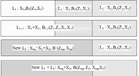
For a multi-layer (more than two) shield, NARMER-1 uses an iterative process that replaces, from source to calculation point, two layers by an equivalent layer. First, the equivalent atomic number is determined by using a neural network trained on large training set. This equivalent atomic number is the closest to a solution to equation (8), where Z is the unknown quantity.
(, , + ) = ,(, , ) (8)
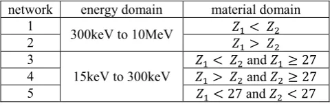
As shown by Table 1, the neural network is divided into five regions that are delimited with respect to physical considerations about sharp variations of induced by fluorescence [5].
Table 1. Description of the five neural networks.
Then, the equivalent thickness () of the equivalent material is calculated to reproduce, with the material, the double-layer build-up, by solving equations (9) where X is the unknown quantity.
(, , ) = ,(, , ) (9)
The above requirements are summarized in equations (10).
H(, , ) = ,(, , ) ≃ +
(10) network energy domain material domain
1
300keV to 10MeV <
2 >
3
15keV to 300keV
< and ≥ 27
4 > and ≥ 27
If is a good approximation, is close to + .
Hence, considering a multi-layer shield composed of N layers, the iterative process starts with the first steps shown by Fig. 1.
Fig. 1. Determination of a three layer shield build-up factor.
2.4 Source integration
For a source S distributed over energy and space, the response
N
O described by a response functionA
O()
to be calculated follows the equation (11).NO(P⃗) = Q ?R STU
SVW
Q ?P⃗R
.
YZ
[(R, P⃗) AR O() [(P⃗, R R)
→ P⃗)] O[(P⃗, R R) → P⃗)] (11)
NARMER-1 uses a Monte Carlo method to integrate points-kernel with build-up factor over the source domain. Considering the spatial and energy meshes defining the source, the code performs a stratified sampling as variance reduction technique. New sampling points are added in each cell proportionally to the variance of the cell, until the variance on the global result reaches the asked precision.
2.5 Computed physical quantities
The following response functions are available in NARMER-1 calculations: uncollided flux, ambient dose equivalent rate H*(10), energy fluence, and air KERMA.
Continuous energy and multi-group cross sections come from JEF2.2. Conversion coefficients from fluence to dose equivalent rate and air KERMA come from
ICRP74 [11].
3 Generic features
3.1 Programming language, computer platforms
NARMER-1 has been developed in C++. It takes advantage of the principles of object oriented design, especially the open/closed principle making future developments easier. It uses python as the user interface. It is currently developed on Linux system but is maintained and available on both Linux and Windows.
3.2 Geometry package
NARMER-1 comes with the TRIPOLI-4® native geometry package, allowing for both a pure surface-based representation, and a combinatorial representation with predefined shapes and boolean operators (any combination of these two kinds of representations can be adopted).
As well as TRIPOLI-4®, NARMER-1 has been also made compatible with any geometry developed in the format of the ROOT software (Brun and Rademakers, 1997). This allows the user to directly use (without recompiling) an already built ROOT geometry.
More generally, NARMER-1 may be linked to any third-party geometry module providing an Application Programming Interface for the current particle position and the next intersection in the direction of flight.
Details concerning visualization tools for building and checking the geometry will be provided in Section 4.
3.3 Sources description
Sources are defined with an energetic spectrum and an emitting volume according to a mesh at a given position.
3.3.1 Energy Distribution
Line spectrum can be used as well as group spectrum based on a 195 bounds pre-defined mesh.
3.3.2 Spatial Distribution
Volume based sources can be described using the following type of meshes: Cartesian, Spherical, Cylindrical, Conic, Toroidal, General Conic, Constant Width Conic, and General Cylindrical.
Surface based sources can be described using the following type of meshes: Cartesian, Spherical Shell, Cylindrical Shell, Disk, Conic Shell, and Toroidal Shell.
4 Specific or recent capabilities
4.1. Exclusion sphere
In order to perform computations for some detectors that can be very close to the emitting volume or inside the emitting volume, it is necessary to avoid a singularity due to the 1/r² factor that can lead to infinite variance. Therefore the code uses an exclusion sphere. The radius of the sphere can be set by the user.
4.2 Tetrahedral meshes
meshes for the definition of emitting volumes. Observed performances of the sampling method allow computation in good conditions.
Fig. 2. A detector point at z=0 in front two emitting meshes, a tetrahedral mesh in the region z>0 and a cartesian mesh in the
region z<0
As an illustration also allowing some considerations about verification and validation, the simple test case Fig. 2 shows a detector point belonging to a median plan defined by z=0 separating two identical emitting volumes having the form of a parallelepiped. The emitting volume in the region z>0 is described by a tetrahedral mesh and the one in the region z<0 is described by a cartesian mesh. NARMER-1 detailed results show that the geometrical intensity is identical for both emitting volumes, and also that the contribution to the global result is close to 50% for each source.
4.3 Double Energy Angle Differential Albedos
Lacunar media shielding studies can be dealt with albedo concept which is an alternative to the "exact" transport method calculations (SN, Monte Carlo). For multiple reflections on lacunar medium walls, one needs double energy-angle differential albedos because they are function of the incident energy. Reflection feature is a point of interest for EDF sponsor. R&D development and validation studies in this domain are still under progress at SERMA.
4.4 Parallel operations
Complex 3D scenes with a high number of gamma sources and a lot of geometrical volumes to cross can lead to substantial simulation times. Therefore, some developments and validation studies are currently under progress to use multi-threads algorithms.
5 Verification and Validation
Since the NARMER-1 code is attended to be used for radiation protection purposes, verification and validation are crucial issues. Verification is supported in particular
by non-regression testing. Excellent results are observed about non-regression results with respect to MERCURE-6. Validation is based on comparison with calculations performed with the TRIPOLI-4® Monte Carlo code as well as with experimental benchmarks.
Here are presented four cases illustrating the validation aspect: two basic tests and two realistic cases in which the ambient dose equivalent rate H*(10) is calculated with NARMER-1 and confronted with TRIPOLI-4® results.
The definition of the geometry is common for both types of calculation.
The relative difference of H*(10) of NARMER-1 from TRIPOLI-4® is defined by equation (12):
N@_. `iAA.j∗()
= N@mn_pqsuvu− N@mn_pwuxyz{x}® N@mn_pwuxyz{x}®
(12)
5.1 Basic configurations
5.1.1 Multi-layers configuration
In this case, a point-like source is surrounded by six concentric spherical screens (from the centre to the outer blanket: Al - Cu - Al - Zr - Cu - Zr). Calculations were done for the following discrete values of energy: 1 MeV, 0.4 MeV, 0.32 MeV, 0.3 MeV, 0.295 MeV, 0.2 MeV and 0.1 MeV.
The ambient dose equivalent rate H*(10) is calculated at six points located at 7.5 cm, 12.5 cm, 17.5 cm, 22.5 cm, 27.5 cm and 32.5 cm from the source represented by dots in Fig. 3.
Fig. 3. Radial cut view of the multi-layers configuration.
The TRIPOLI-4® calculations concerned the transport of rays only. Variance reduction technique was required for the 0.1 MeV source in order to converge.
Fig. 4 whereas H*(10) numerical values of NARMER-1 calculations are shown in Table 2.
Fig. 4. Relative difference of H*(10) NARMER-1 calculations with respect to TRIPOLI-4® calculations for the multi-layers configuration.
Above 300 keV of energy, the relative difference does not exceed 10%. However, below 300 keV, NARMER-1 results overestimate TRIPOLI-4® significantly. We note that 300 keV represents the cut energy in the definition of the neural networks domains used to determine the equivalent atomic number of the fictive layer for build-up calculations (see Table 1). Cu is replaced by Fe in the material list of the double-layer build-up formula. The back-scattering flux is overestimated in the third layer (Al) due the heavier material (Zr) in the fourth layer. This test case uses multiple times the iterative process (Fig. 1).
Table 2. Numerical results of NARMER-1 for H*(10) calculations (μSv/h) of a multi-layers configuration
(convergence criteria is 1%).
(cm) 1 MeV 0.4 MeV 0.32 MeV 0.3 MeV 7.5 9.778E-05 4.867E-05 4.025E-05 3.821E-05 12.5 2.694E-05 1.001E-05 7.209E-06 6.598E-06 17.5 1.112E-05 3.658E-06 2.482E-06 2.276E-06 22.5 4.643E-06 9.907E-07 5.715E-07 6.250E-07 27.5 2.187E-06 3.419E-07 1.677E-07 1.803E-07 32.5 1.030E-06 1.105E-07 4.565E-08 4.611E-08
0.295 MeV 0.295 MeV 0.1 MeV 7.5 3.747E-05 2.561E-05 1.072E-05 12.5 6.359E-06 2.916E-06 1.555E-07 17.5 2.174E-06 8.218E-07 8.457E-09 22.5 5.893E-07 1.455E-07 9.245E-11 27.5 1.667E-07 2.270E-08 1.933E-13 32.5 4.180E-08 3.199E-09 3.827E-16
5.1.2 Simplified water pipe
This case corresponds to a 0.1 cm thick, 8.1 cm outer radius, 200 cm high, steel pipe filled with water.
A point-like source is located at the pipe’s centre with three different energies: 10 MeV, 1 MeV and 0.1 MeV.
The ambient dose equivalent rate H*(10) is calculated at three locations distant from the source of 5 cm (in the water), 8.05 cm (in the steel) and 9 cm (in the air). These locations are represented by dots in Fig. 5.
Fig. 5. Radial cut view of a simplified water pipe.
The whole electromagnetic cascade has been taken into account for the 10 MeV while only rays have been transported for the 1 MeV and 0.1 MeV sources in the TRIPOLI-4® calculations.
Results of the H*(10) relative difference as defined by equation (12) are shown for different energy source as a function of the distance from the source in Fig. 6 whereas H*(10) numerical values of NARMER-1 calculations are shown in Table 3.
Fig. 6. Relative difference of H*(10) from NARMER-1 to TRIPOLI-4® for the simplified water pipe configuration.
It can be seen that the relative difference remains below about 10% in all cases which reflects the good agreement between the two codes.
Table 3. Numerical results of NARMER-1 for H*(10) calculations (μSv/h) of a simplified water pipe configuration
(convergence criteria is 1%).
5. 8.05 9.
10 MeV 1.158E-02 4.296E-03 3.418E-03
1 MeV 2.383E-03 8.771E-04 6.949E-04
5.2 Realistic configurations
5.2.1 Water pipe with protection
This case corresponds to a realistic water pipe which is made of a hollow steel cylinder (inner radius 30 cm, 2 cm thick) full of water which is covered by a 4 cm thick lead layer.
The source is distributed on the volume of the water and takes several discrete values (7 MeV, 3 MeV, 1 MeV and 0.6 MeV).
The ambient equivalent dose is calculated at different distances from the centre of the pipe: 30 cm (interface water/steel), 32 cm (interface steel/lead), 36 cm (interface lead/air), and in the air at 40 cm, 45 cm, 50 cm, 55 cm, 60 cm, 80 cm and 90 cm represented by dots in Fig. 7.
Fig. 7. Radial cut view of the water pipe with protection.
The full electromagnetic cascade has been taken into account for the TRIPOLI-4® calculations for the 7 MeV and 3 MeV sources. Only rays have been transported for the two others energy source.
Fig. 8. Relative difference of H*(10) NARMER-1 calculations with respect to TRIPOLI-4® calculations for the configuration of a water pipe with protection.
The difference between NARMER-1 and TRIPOLI-4® is between -7% and +18%. This difference does not vary linearly with the source energy because of different physical effects: Compton effect is dominant at low energy whereas at high energy pair creation can occur.
Table 4. Numerical results of NARMER-1 for H*(10) calculations (μSv/h) of a water pipe with protection (convergence criteria is 1%).
cm 7 MeV 3 MeV 1 MeV 0.6 MeV 30 1.183E+00 6.066E-01 2.490E-01 1.651E-01 32 5.579E-01 2.581E-01 6.812E-02 3.112E-02 36 4.942E-02 2.288E-02 1.123E-03 2.773E-05 40 4.334E-02 2.020E-02 9.948E-04 2.469E-05 45 3.829E-02 1.771E-02 8.757E-04 2.187E-05 50 3.416E-02 1.577E-02 7.812E-04 1.954E-05 55 3.068E-02 1.425E-02 7.048E-04 1.767E-05 60 2.788E-02 1.294E-02 6.467E-07 1.617E-05 80 2.028E-02 9.455E-03 4.780E-04 1.199E-05 90 1.761E-02 8.241E-03 4.222E-04 1.069E-05
5.2.2 UO2 - PuO2 source
A cylinder of PuO2-UO2, in which the source is equally distributed, is located in front of a series of screens as drawn on Fig. 9.
Fig. 9. Radial cut view of the UO2-PuO2 configuration.
The configuration of the series of 40 cm long screens is defined as following:
A 1 cm thick, 10 cm tall, iron screen is located at 28.5 cm from the center of the source,
A 5 cm thick, 17 cm tall, Kyowa-glass screen is located at 30 cm from the center of the source A 0.9 cm thick, 17 cm tall, glass screen is
located at 30 cm from the center of the source close to a 0.8 cm thick, 17 cm tall, leaded glass screen situated at 30.9 cm from the center of the source.
Fig. 10. Energy distribution of the γ source.
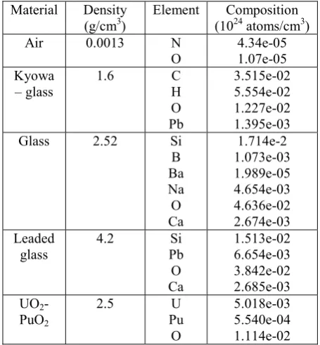
The atomic compositions are noted in the Table 5.
Table 5.Atomic compositions of the UO2-PuO2 test case
Material Density (g/cm3)
Element Composition (1024 atoms/cm3)
Air 0.0013 N
O
4.34e-05 1.07e-05 Kyowa
– glass
1.6 C
H O Pb 3.515e-02 5.554e-02 1.227e-02 1.395e-03
Glass 2.52 Si
B Ba Na O Ca 1.714e-2 1.073e-03 1.989e-05 4.654e-03 4.636e-02 2.674e-03 Leaded glass
4.2 Si
Pb O Ca 1.513e-02 6.654e-03 3.842e-02 2.685e-03 UO2
-PuO2
2.5 U
Pu O
5.018e-03 5.540e-04 1.114e-02
The ambient dose equivalent rate H*(10) is calculated at three points, respectively at coordinates (50.,0.,-10.), (50.,0.,0.) and (50.,0.,10.), symbolized by dots in Fig. 9. The Table 6 presents the results of the calculations made with NARMER-1 and TRIPOLI-4® and their comparison.
Table 6. H*(10) calculated with NARMER-1 and TRIPOLI-4®
z
NARMER-1 TRIPOLI-4® DevH*(10)
(N-T)/T (%) H*(10) (μSv/h) H*(10) (μSv/h) 10. 0. -10. 1.55e+03 2.10e+03 1.93e+03 0.12 0.19 0.14 1.29e+03 1.66e+03 1.54e+03 0.04 0.07 0.05 19.7 26.8 25.6
NARMER-1 values overestimate TRIPOLI-4® values of about 20%.
6 Visualization and pre-treatment
Sharing the same geometry package as TRIPOLI-4®, NARMER-1 can be used with the pre-and-post treatment tool distributed with TRIPOLI-4®, known as “Visualizer T4G”. The user also has possibility to check the definition of the geometry by using the last verification tools implemented in TRIPOLI-4®, including “Check Geom” and “Check Tracking” functionalities.
7 Summary and conclusion
NARMER-1 is a simplified code that allows to perform fast calculations to evaluate ambient dose equivalent H*(10) and KERMA for radiation protection studies.
A validation study has been done with comparison to TRIPOLI-4® considered as a reference code.
Basic configurations and sophisticated configurations show overall a good agreement between the two codes. In some cases, we observe an overestimation of NARMER-1 with respect to TRIPOLI-4®. The results are conservative for radiation protection studies.
NARMER-1 calculations are much faster than TRIPOLI-4® ones: NARMER-1 calculations last less than one minute and can reach several minutes for complicated configurations. These calculations times remain orders of magnitude below those met for TRIPOLI-4®.
Acknowledgments
The authors gratefully acknowledge EDF for its support to the NARMER-1 project.
References
[1] C. Devillers, "Programme MERCURE-3, Atténuation en ligne droite dans une géométrie à trois dimensions", Internal Report, CEA-R 3264 (1967)
[2] C. Devillers, C. Dupont, “MERCURE-4 – Three Dimensional Monte-Carlo Program for the integration of line of sight point attenuation kernels”, Internal Report, CEA-N-1726 (1974)
[3] C. Dupont, "MERCURE-5.3 : Un Programme de Monte-Carlo à trois dimensions pour l'intégration de noyaux ponctuels d'atténuation en ligne droite.", Internal Report, Rapport DMT 95/552 SERMA/LEPP 95/1817 (1995)
[4] A. Assad, M. Chiron, J.-C. Nimal, C.M. Diop, and P. Ridoux, “General Formalism for Calculating Gamma-Ray Buildup Factors in Multilayer Shields into MERCURE-6 Code”, Jour. Nuc. Sci. and Tech., Supplement 1, p. 493- 497 (March 2000)
[5] C. Suteau, M. Chiron, “Improvement of MERCURE-6 General Formalism for calculating gamma-ray build-up factors in multilayer shields”, Nucl. Sci. Eng., 147, 43-55, (2004)
[6] L. Bourdet, Internal Report, Rapport DMT 95/482 SERMA/LEPP 95/1796 (1995)
Petit, J.C. Trama, T. Visonneau, A. Zoia, “TRIPOLI-4®, CEA, EDF and AREVA reference Monte Carlo code”, Annals of Nuclear Energy, 82 (2015) 151–160.
[8] R. E. Alcouffe, F. W. Brinkley, D. R. Marr, and R. D. O’Dell, “User’s Guide for Twodant: A Code Package for Two-Dimensional, Diffusion-Accelerated, Neutral-Particle, Transport”, LA-10049-M, Revised, Vol. 1, p. 1, Group X-6, Los Alamos National Laboratory (Nov. 1989).
[9] S. Kitsos, C. M. Diop, A. Assad, J. C. Nimal, and P. Ridoux, “Improvement of Gamma-Ray Sn Transport Calculations Including Coherent and Incoherent Scatterings and Secondary Sources of Bremsstrahlung and Fluorescence: Determination of Gamma-Ray Buildup Factors”, Nucl. Sci. Eng, 123, 215-227 (1996) [10] The JEF-2.2 Nuclear Data Library, NEA JEFF Report 17 (2000).