Bayesian Magic in Asteroseismology
T. Kallinger1,a
Institute for Astronomy, University of Vienna, T¨urkenschanzstrasse 17, 1180 Vienna, Austria
Abstract. Only a few years ago asteroseismic observations were so rare that scientists had plenty of time to work on individual data sets. They could tune their algorithms in any possible way to squeeze out the last bit of information. Nowadays this is impossible. With missions like MOST, CoRoT, andKeplerwe basically drown in new data every day. To handle this in a sufficient way statistical methods become more and more important. This is why Bayesian techniques started their triumph march across asteroseismology. I will go with you on a journey through Bayesian Magic Land, that brings us to the sea of granulation background, the forest of peakbagging, and the stony alley of model compar-ison.
1 Introduction
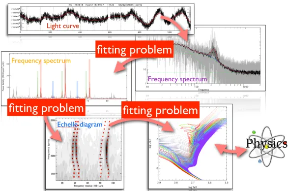
Asteroseismology is the study of the interior of stars by the observation and analysis of oscillations at their surface [Oxford English Dictionary]. In practice this often comes down to that one has to compare observations of a star to a model to learn something about the star or even physics in general. For solar-type oscillator a frequently used strategy to get there is outlines in Fig. 1.
Fig. 1.Schematic view of an “ideal” asteroseismic analysis: from the lightcurve to testing physics includes mod-elling the instrincis background signal, extracting the mode parameters, and a model comparison, all of which are classical fitting problems.
a e-mail:[email protected] /
C
Owned by the authors, published by EDP Sciences, 2015 / 101
Along this road at least 3 steps involve classical fitting problems, i.e. the need to parameterise the observations with a realistic model and to infer its best-fit parameters, preferably also with realistic uncertainties. While for individual data sets this appears to be straight forward it turned out to be a big challenge after theSpace Photometry Revolution. MOST, CoRoT, andKeplerhave delivered tens of thousands of high-precision lightcurves and (apart from the occasional analysis of individual data sets) it is no longer feasible to analyse them on a ‘star-by-star’ basis. Statistically solid tools are required to find models that represent the observations best (with the model complexity being driven only by the data) and the best possible model parameters (with uncertainties that realistically reflect the errors of the measurements).
A promising solution to this problem is provided by probability theory (a good summary may be found in [1]). There are 2 (and only 2!) rules to spawn all of probability theory:
– Product rule:P(A,B|C) = P(A|C)P(B|A,C), which gives the probability of proposition AandB
givenC
– Sum rule:P(A+B|C)=P(A|C)+P(B|C)−P(A,B|C), which gives the probability of proposition
AorBor both givenC
From the product rule follows Bayes’ Theorem,P(A|B,C)=P(A|C)P(B|A,C)/P(B|C), which allows to compute the probability of propositionAgivenB(andC) from the probability of propositionBgiven
A(andC) and therefore relates current to prior evidence. A probabilistic (often called “Baysian”) anal-ysis simply uses these theorems to determine the probability of propositions (i.e., parameter values, models, hypotheses, etc.) and thereby provides:
– a quantitative approach to scientific inference, which allows to determine model parameters and their uncertainties.
– a consistent and correct way to normalise probabilities, which allows to evaluate different models (and therefore the physics they are based on).
– marginalisation, which is a consequence of the sum rule that allows to marginalise “unwanted” parameters via integrating them out asP(θ0, . . . , θn−1|M,D,I)=
P(θ0, . . . , θn|M,D,I)dθn
2 Applications of “Bayesian Magic”
In the following three examples are show for a Bayesian stastics in asteroseismology.
2.1 Stellar background modelling
The brightness variations of a star with a convective envelope (i.e., basically all stars withTeff
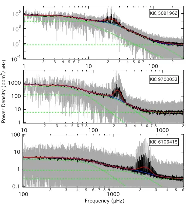
7000K) are due to various physical phenomena. While on long timescales the signal reflects rotational modulation and magnetic activity, short timescales are dominated by granulation and solar-like oscil-lations. The power density spectrum (PDS) of such a star has therefore a characteristic global shape. The quasi-stochastic granulation signal produces a frequency dependent “noise” (with decreasing am-plitudes towards higher frequencies), which is superposed by a regular pattern of oscillation modes. Their amplitudes are approximately modulated by a Gaussian centred on the peak frequencyνmax(see Fig. 2). To disentangle these components one needs to model the granulation signal. Even tough fitting the granulation background is a relatively low-dimensional problem, there was no consensus on neither the functional form of the model nor the number of components needed to represent the observations best [2–4]. As a consequence assuming different models may not only result in different granulation parameters [5] but also sensibly affect the subsequent frequency analysis [6].
Besides linear or exponential approximations a model of the formP(ν)∝iξσ2iτi/[1+(2πντi)
ci] is
most commonly used, whereτis the characteristic granulation timescale andξa factor that normalises
μ
!!"
#
μ
$%&
$%&
$%&
Fig. 2.Power density spectra of three stars at different evolutionary stages (top: high up the RGB; middle: at the buttom of the RGB; bottom: on the main sequence), showing that all timescales and amplitudes (granulation as well as pulsation) scale simultaneously. Grey and black lines indicate the raw and heavily smoothed spectrum, respectively. The global fit is shown with (red) and without (blue) the Gaussian component. Green lines indicate the individual background and white noise components of the fit.
shown thatc=4 seems to be more appropriate butcis also frequently left a free parameter in the fit leading to a large variety of exponents.
Driven by this unclear situation [7] carried out a detailed Bayesian analysis of various granulation background models for a large sample ofKepler stars covering evolutionary stages from the main sequence to high up the giant branch. They found that in the vicinity of the oscillation power excess (about 0.1–10×νmax) a 2-component model with a free exponent (which turns out out to be close to 4) formally fits the observations best. However, they also found that even the high-precisionKepler
data are not long enough to provide enough evidence to constrain the exponent from the data and that a similar model with the exponent fixed to 4 reproduces the observations equally well. Furthermore, they establish that the model is universal (i.e., appropriate for all evolutionary stages) and that the specific choice of the background model can affect the determination ofνmax, introducing systematic
uncertainties to asteroseimically determined fundamental parameters.
2.2 Peak bagging
Peak bagging refers to the parameter determination of solar-like oscillations. It can be shown that the limit power spectral density of a series of solar-like oscillation modes follow a sequence of Lorenztian profiles,P(ν) = iai2(πΓi)−1/[1+4(ν−νi)2/Γ2i], whereai,νi, andΓicorrespond to the amplitude,
central frequency, and linewidth (which relates to the oscillation lifetimeτ, byΓ=(πτ)−1) of thei-th mode. In case of rotation, the profiles of nonradial modes are split into 2l+1 multiplet components [8], withlbeing the spherical degree of the mode. The individual components are thereby separated by the star’s angular velocity and their amplitudes scale with the inclination of the rotation axis. The profile of a single (nonradial) mode can therefore require up to 5 parameters to be fit (assuming symmetrically split multiplets).
μ
μ
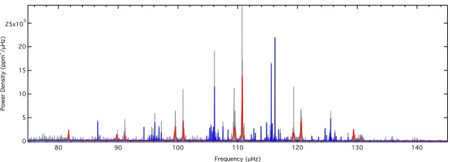
Fig. 3.Peak bagging result for the red giant KIC3744043. The red and blue lines indicate sequences of Lorenztian profiles and sinc functions fitted tol=0, 2 andl=1 modes, respectively.
consecutive modes per radial order (see Fig. 3). Since the lifetime of these modes are quite long (up to several hundred days) they are often not resolved so that a sinc function is more appropriate to fit them (which reduced the number of free parameters from 3 to 2 per individual mode). After all, even the oscillation spectrum of red giants can easily add up to more than a hundred free parameters to be fit.
To exploit the full potential of asteroseismology requires to extract the full information contained in the oscillation spectrum. For such a high-dimensional problem, however, sophisticated and robust analysis tools are indispensable. Bayesian statistics provides the perfect environment to tackle such a task but has only made its way into asteroseismology a few years ago. Early attempts were made by, e.g., [9] or [10]. Recent developments, like the Bayesian nested sampling tooldiamonds[11] (see also
an article in this proceedings), do now allow to automatically analyse complex oscillation patterns with little risk of over-fitting the data. Automation is also a big topic in the analysis of red giants.
Keplerdelivered more than 13 000 light curves of red giants, which can only be fully examined with fast automated tools. I am working on an algorithm specifically designed to reliably extract mode parameters (and their uncertainties) from red-giant oscillation spectra. It scans the spectrum for sta-tistically significant peaks, performs an automatic mode identification and fits Lorentzian profiles to radial, resolved dipole, and quadruple modes and sinc functions to unresolved dipole modes (including rotational splittings) using the Bayesian nested sampling algorithm MultiNest[12].
2.3 Grid modelling
The final step on our road to asteroseismology is called grid modelling. This is usually done by com-puting the theoretical eigenfrequencies of large grids of stellar models and searching those grids for the pulsation model that most closely reproduce the observed frequencies. As the eigenfrequencies reflect the physical properties of a star it should therefore help to improve our knowledge about stellar interiors.
In the past,χ2-minimization techniques [13] (i.e., minimizing the difference between observed and model frequencies) have been used to search for a best fit. This approach, however, assumes that the theoretical frequencies are free of systematic uncertainties but it is know that stellar surface layers, rotation, and magnetic fields imprint erratic frequency shits, trends, and other non-random behaviour in the frequency spectra. Most prominently, insufficient modelling of the outer convective layers cause the model frequencies at high radial orders to differ from the observations (see Fig. 4) and therefore hamper a direct comparison. This so-calledsurface effectcan be “corrected” through calibration for the Sun [14] but it seems unlikely that the solar calibrated surface correction is universally applicable. So in the best case it reduces the problem but does not solve it.
Fig. 4.Non-adiabatic (shaded symbols) and adiabatic (open symbols) frequencies of the most probable solar model from evaluating the BiSON frequencies (black circles+error bars). The figure is taken from [15] and shows the solar surface effect.
model frequency (νi,m) asP(νi|MΔj,I) ∝ exp[−(νi,o −νi,m−Δi)2/2σ2i], where they allow for an
un-known systematic deviationΔi. By using marginalisation,Δican now be integrated out asP(νi|Mj,I)=
Δi,max Δi,min P(νi|M
Δ
j,I)δΔi, without the need to know its exact value. Thus by simply defining some
bound-aries for the surface effect one gets the correct probability, which is then combined asP(D|Mj,I) =
iP(νi|Mj,I) to compute the probability that a given pulsation model matches a set of observed
fre-quencies. A similar formalism can be used to account for an unknown mode identification (which is particularly problematic in the presence of rotational splittings) or the finite grid resolution.
In fact, the above approach can not only correctly treat the surface effect, it actually allows us to measure it in different stars. [16] analysed a set of solar-likeKeplertargets and found that the magni-tude of the surface effect depends on the mixing length parameter of the best-fit model. Furthermore they found that some stars in their sample do not show a surface effect at all, while the most significant surface effects are measured for stars that are close to the Sun’s position in the Hertzsprung-Russel diagram (see Fig. 5).
3 Conclusions
Use the power of evidence!!!
References
1. E.T. Jaynes, G.L. Bretthorst, eds., Probability theory : the logic of science
(Cambridge University Press, Cambridge, UK, New York, 2003) 0-521-59271-2, http://opac.inria.fr/record=b1099730
2. J. Harvey,High-resolution helioseismology, inFuture Missions in Solar, Heliospheric&Space Plasma Physics, edited by E. Rolfe, B. Battrick (1985), Vol. 235 ofESA Special Publication, pp. 199–208
Fig. 5.HR diagram for 23 stars observed byKeplerwith the symbol color indicating the “strenght” of the mea-sured surface effect. The figure is taken from [16].
4. C. Karoff, T.L. Campante, J. Ballot, T. Kallinger, M. Gruberbauer, R.A. Garc´ıa, D.A. Caldwell, J.L. Christiansen, K. Kinemuchi, ApJ767, 34 (2013)
5. S. Mathur, S. Hekker, R. Trampedach, J. Ballot, T. Kallinger, D. Buzasi, R.A. Garc´ıa, D. Huber, A. Jim´enez, B. Mosser et al., ApJ741, 119 (2011)
6. T. Appourchaux, H.M. Antia, O. Benomar, T.L. Campante, G.R. Davies, R. Handberg, R. Howe, C. R´egulo, K. Belkacem, G. Houdek et al., A&A566, A20 (2014)
7. T. Kallinger, J. De Ridder, S. Hekker, S. Mathur, B. Mosser, M. Gruberbauer, R.A. Garc´ıa, C. Karoff, J. Ballot, A&A570, A41 (2014)
8. L. Gizon, S.K. Solanki, ApJ589, 1009 (2003)
9. M. Gruberbauer, T. Kallinger, W.W. Weiss, D.B. Guenther, A&A506, 1043 (2009)
10. O. Benomar, F. Baudin, T.L. Campante, W.J. Chaplin, R.A. Garc´ıa, P. Gaulme, T. Toutain, G.A. Verner, T. Appourchaux, J. Ballot et al., A&A507, L13 (2009)
11. E. Corsaro, J. De Ridder, A&A571, L13 (2014)
12. F. Feroz, M.P. Hobson, M. Bridges, MNRAS398, 1601 (2009) 13. D.B. Guenther, K.I.T. Brown, ApJ600, 419 (2004)
14. H. Kjeldsen, T.R. Bedding, J. Christensen-Dalsgaard, ApJL683, L175 (2008) 15. M. Gruberbauer, D.B. Guenther, T. Kallinger, ApJ749, 109 (2012)