HIGH-FREQUENCY METHOD ANALYSIS ON
SCATTERING FROM HOMOGENOUS DIELECTRIC OBJECTS WITH ELECTRICALLY LARGE SIZE IN HALF SPACE
X. F. Li, Y. J. Xie, and R. Yang
National Laboratory of Antennas and Microwave Technology Xidian University
P.O. Box 223, Xi’an 710071, Shannxi, P. R. China
Abstract—The high-frequency method for solving the scattering from homogeneous dielectric objects with electrically large size in half space is presented in this paper. In order to consider the scattering fields of the targets in half space, the half-space physical optics method is deduced by introducing the half-space Green’s function into the conventional physical optics method (PO). Combined with the graphical-electromagnetic computing method to read the geometry information of all visible facets, the equivalent currents and the reflection coefficients are utilized to account of the homogenous dielectric objects with half-space physical optics method in half space. The numerical results show that this method is efficient and accurate.
1. INTRODUCTION
Numerous authors have derived a variety of methods which are used for computing the high-frequency radar cross section (RCS) of complex radar targets in half space. The scattering fields of the targets in half space could be computed by using the Finite element method (FEM) [8], Finite-difference time-domain methods (FDTD) [9], but they cause some difficulties in the solution procedure [12]. Some researchers try to combine the half-space Green’s function and the Method of moment (MOM) to consider the electrically large targets in half space [10–12], but it also requires more mass storage memory, which results in lower processing speed and computational efficiency. In this paper, based on the analysis of the electrically large conductive targets in half space [13], we have further introduced the high-frequency method into the homogeneous dielectric object with electrically large size in half space.
This paper focuses on the prediction of radar cross section of homogeneous dielectric object with electrically large size in half space. In order to consider the scattering fields of the electrically large target in half space, the half-space physical optics method (PO) for dielectric object is obtained by introducing the half-space Green’s function into the PO method for dielectric object. Combined with the graphical-electromagnetic computing (GRECO) method, the shadow regions are eliminated by displaying lists technology of OpenGL to rebuild the target, and the geometry information is attained by reading the color and depths of each pixel [4]. The results show that the half-space physical optics method for dielectric objects is efficient and accurate. For illustration purposes, we limit our presentation to the monostatic case for homogeneous dielectric objects with electrically large size in half space.
2. THEORY
Consider an arbitrarily shaped dielectric object illuminated by a plane wave in the half space, surfacesis assumed to represent a closed surface of target. The far zone scattering electric and magnetic fields of the homogenous medium in half space can be expressed as:
Es
r = −jωAr− ∇Ve−
1
ε0∇ ×
F, r ∈S (1)
Hs(r) = −jωF(r)− ∇Vm+
1
µ0∇ ×
A, r ∈S (2)
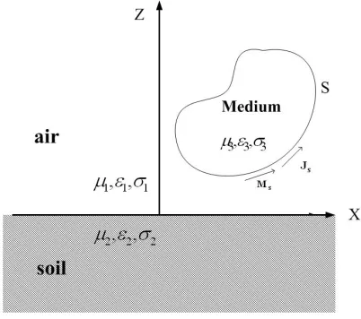
As show in Fig. 1, in order to solve the scattering fields of the homogenous dielectric object with electrically large size in half space, the half-space Green’s function is introduced into the physical optics method to calculate the contributions of scattering between the target and the ground plane.
Figure 1. The reflected field of the ground and target in half space.
It is permissible to express the vector and the scalar potentials as follows [14]:
A(r)=µ0
S
¯
GA
r, r·JrdS (3)
Ve(r)= −
1
jωε0
S
Gqex r, r∂Jx ∂x +G
qe y
r, r∂Jy ∂y +G
qe z
r, r∂Jz ∂z
dS (4)
F(r)=ε0
S
¯
GF
r, r·MrdS (5)
Vm(r)= −
1
jωµ0
S
Gqmx r, r∂Jx ∂x +G
qm y
r, r∂Jy ∂y +G
qm z
r, r∂Jz ∂z
dS (6)
wherer andr represent the position vectors for the observation point and the increment area dS, respectively, and u0 and ε0 denote the
2.1. The Half-Space Green’s Function
The half-space Green’s function can be impressed by the vector and scalar potentials, and the vector potential is not uniquely specified. In this paper, we express it as follows [14]:
¯
GA = (ˆxˆx+ˆyˆy)GxxA +ˆzˆxG zx
A +ˆzˆyG zy
A +ˆzˆzG zz
A (7)
¯
GF = (ˆxˆx+ˆyˆy)GxxF +ˆzˆxG zx
F +ˆzˆyG zy
F +ˆzˆzG zz
F (8)
with
GyyA = GxxA, Gqey =Gqex (9)
GyyF = GxxF , GqeF =GqeF (10)
where GxxA, GzxA, GzyA and GzzA denote the spatial domain half-space Green’s function for the electric vector potentials; Gqex , Gqey and Gqez
denote the spatial domain half-space Green’s function for the electric scalar potentials; GxxF , GzxF , GzyF and GzzF denote the spatial domain half-space Green’s function for the magnetic vector potentials; Gqmx ,
Gqmy , Gqmz denote the spatial domain half-space Green’s function for the magnetic scalar potentials. The detailed accounts of derivations are beyond the scope of this paper. Please see [15, 16] for a full derivation. The main formulations are presented as follows:
GxxA = µ 4π −j 2 +∞ −∞ kρ kz
H0(2)(kρρ) e−jkz|z−z
|
+Aehe−jkzz
dkρ (11)
GzxA =−µ 8π ∂ ∂x +∞ −∞ kρ kz
H0(2)(kρρ)
kz k2 ρ
(Che−Aeh)e−jkzz
dkρ (12)
Gqex =− j 8πε
+∞
−∞ kρ kz
H0(2)(kρρ)
e−jkz|z−z|+k
2Ae h+k
2 zChe k2
ρ
ejkzz
dkρ (13)
GzzA= µ 4π −j 2 +∞ −∞ kρ kz
H0(2)(kρρ) e−jkz|z−z
|
+Aeve−jkzz
dkρ (14)
Gqez = 1 4πε −j 2 +∞ −∞ kρ kz
H0(2)(kρρ) e−jkz|z−z
|
+Cvee−jkzz
dkρ (15)
with
Aeh = RTEe−jkzz, Ce
h=−RTMe−jkzz
(16)
Aev = RTEe−jkzz, Ce
v =−RTMe−
jkzz (17)
whereRTE, RTM are Fresnel reflection coefficient, kx, ky, kz are the
wavenumbers of x, y, z in the global coordinate system, respectively.
In order to obtain the half-space Green’s function, we compute the vector and the scalar potentials by the discrete complex image method. Through the Sommerfeld identity, a closed-form spatial Green’s function of a few terms is found from the quasi-dynamic images, the complex images, and the surface waves [15, 16].
To obtain the spatial-domain Green’s functions in closed forms, it would be useful to give the definition of the spatial-domain Green’s function
G= 1 4π
SIP
˜
G(kρ)H (2)
0 (kρ)kρdkρ (18)
where, G and ˜G are the Green’s function in the spatial and spectral domains, respectively. H0(2) is the hankel function of the second kind and SIP is the Sommerfeld integration path.
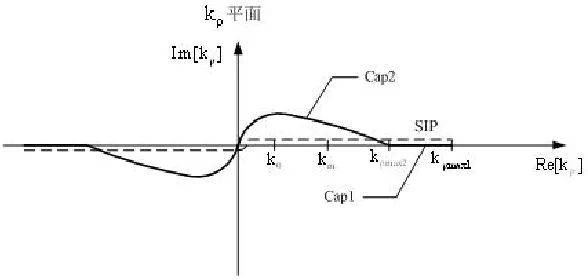
To alleviate the necessity of investigating the spectral-domain Green’s functions in advance and the difficulties caused by the trade-off between the sampling range and the sampling period, the approximation is performed in two levels. The first part of approximation is performed along the pathCap1 while the second part is done along the pathCap2, as show in Fig. 2. The main formulations may refer to [17, 18].
Figure 2. The pathCap1andCap2used in two-level approximation.
2.2. Graphical Processing in Half-Space
plane is obtained by reading the colors and depths of each pixel, and the shadow regions are eliminated by displaying lists technology of OpenGL to rebuild the target.
GRECO method was introduced by Rius in 1993 [3]. It can be integrated with CAD geometric modeling package and high-frequency theory for RCS prediction. By the hardware graphics accelerator, hidden surfaces of the image have been previously removed.
To the fixed screen, the calculation complexity is not varied with the complexity and dimension of targets. The targets are rebuilt by displaying lists technology of OpenGL and hidden surfaces of the image have been previously removed by the hardware graphics accelerator. Then we make use of the resolution to disperse the curve face into pixels that satisfy the requirement of the electromagnetic calculation, meanwhile, the scene is rendered using the Phong local illumination model [3]. For three light sources of purely green, red and blue colors, respectively, located over each one of the three coordinate axis, the three color components (Red, Blue, Green) for this pixel are equal to the (nx, ny, nz) components of the unit normal to surface. Meanwhile,
the depths of each pixel are obtained in the same way. The depth of each pixel is equal to the distance between the observer and each surface element.
Obtaining the unit normal and depth of each illuminated pixel of the target, the radar cross section of homogeneous dielectric object can be exactly calculated with the half-space physical optics method for homogeneous dielectric object below.
2.3. The Half-Space Physical Optics Method for Dielectric Object
The half-space Green’s function has been introduced into the physical optics method to account for the scattering of homogeneous dielectric object with electrically large size in half space. Combined with the GRECO method, the shadow regions have been previously removed by the hardware graphics accelerator, and the geometry information is obtained by reading the color and depths of each pixel.
The total field backscattered field of the targets is summed up from the contributions of all visible facets while for the hidden parts the total fields are assumed to be zero. Based on the physical optics method for dielectric object, the surface currents (Js, Ms) may be expressed as [19]:
Js =
1
z
−ei⊥(i·n)−R⊥es⊥(s·n)
E⊥
+1
z
(n×ei⊥) +R//(n×es⊥)
Ms =
(ei⊥×n) +R⊥(es⊥×n)
E⊥
−ei⊥(n·i) +R//(n·s)
E// (20)
with [20]
R⊥ = η2cosθi−η1cosθt
η2cosθi+η1cosθt
(21)
R// = η1cosθi−η2cosθt
η1cosθi+η2cosθt
(22)
in whichR⊥, R// are the Fresnel reflection coefficients,ηi=
ui/εi is
the wave impedance for mediumi(i= 1,3), respectively.
To apply the far-field approximation, that is, the observation point is located far enough from the scattering object, we could obtain
∇Φ≈jksˆΦ (23) and substitute (3), (4), (5), (23) into the scattered field (1), which leads to the equation:
Es(r) = −jωµ0
S
¯
GA
r, r·JrdS
+ k·sˆ
ω·ε0
s
Gqex ∂ ∂xJ(
r) +Gqey ∂ ∂yJ(
r)
+Gqez ∂ ∂zJ(
r)
dr−jωε0
S
¯
GF
r, r·MrdS (24)
Equation (24) is then calculated for every illuminated facet and the complex RCS due to scattering from every illuminated facet is calculated as [21]:
√
σ = lim
R→∞2
√
πREs·ˆer Eo
exp(jkR) (25)
where exp(jkR) is a phase term that has been introduced into the equation in order to account for the facet location with respect to the global coordinate system, HereR is the position vector for the facet’s reference vertex with respect to the global coordinate system.
3. RESULTS
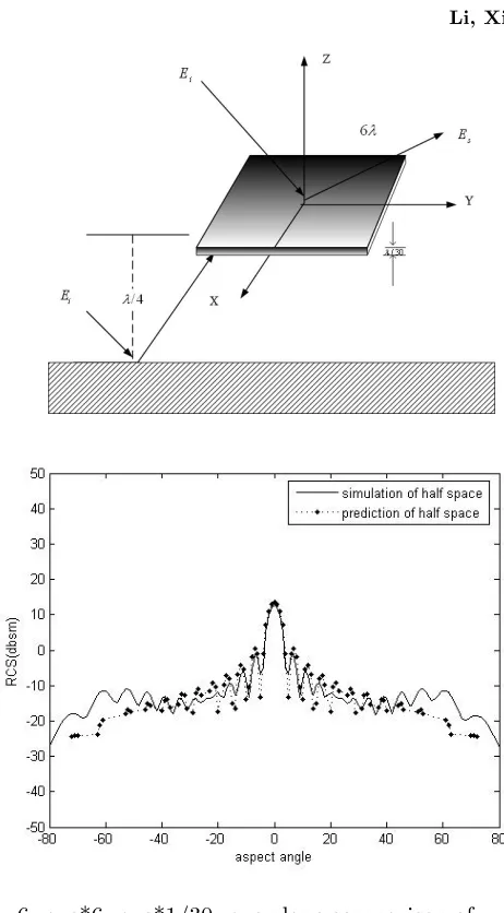
Figure 3. 6wave*6wave*1/30wave plane comparison of prediction and simulation of software in half space, frequency 10 GHz.
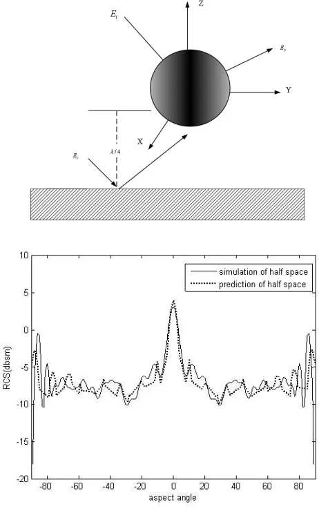
Figure 4. Dielectric sphere comparison of prediction and simulation of software in half space, frequency 10 GHz.
the knowledge of the unit normal at the illuminated surfaces of the targets in half space.
examples below.
Figure 3 shows a dielectric flat plane (6λ×6λ×30λ) is placedλ/4 above the soil. Here,λrepresents the wavelength in the vacuum. The dielectric plane has a relative dielectric permittivityεr = 4.0, relative
magnetic permeability µr = 1.0. The soil has a relative dielectric
permittivity εr = 4.0, relative magnetic permeabilityµr= 1.0
There is good fit between the prediction of the derivated equation and the simulation of ANSOFT HFSS software, except for the flash produced by the leading edge of plate in total prediction. The reason for this discrepancy is caused by the currents that are induced on facet’s free edges.
Figure 4 shows a dielectric sphere is placed λ/4 above the soil. Here, the sphere radius is 5λ and the soil has a relative dielectric permittivity εr = 4.0, relative magnetic permeability µr = 1.0. The
dielectric sphere has a relative dielectric permittivityεr = 4.0, relative
magnetic permeabilityµr= 1.0.
It indicates the predictions are in good agreement with the simulation of software, which proves that the half-space Green’s function applied the physical optics method for dielectric object is accuracy for the targets with large electric dimensions in half space.
4. CONCLUSION
In this paper, we have presented an accurate and powerful approach for calculating the homogeneous dielectric object with electrically large size in half space. In order to consider the scattering fields of the targets in half space, the half-space physical optics method has been deduced by introducing the half-space Green’s function into the conventional physical optics method (PO). Combined with the graphical-electromagnetic computing method to read the geometry information of all visible facets, the equivalent currents and the reflection coefficients were utilized to account of the homogenous dielectric objects with half-space physical optics method in half space. The numerical results have shown that this method is efficient and accurate.
REFERENCES
1. Zhao, Y., X.-W. Shi, and L. Xu, “Modeling with NURBS surfaces used for the calculation of RCS,” Progress In Electromagnetics Research, PIER 78, 49–59, 2008.
3. Fei, Y. and G. Zhu, “Electromagnetic diffraction of a very obliquely incident plane wave field by a wedge with anisotropic impedance faces,” Journal of Electromagnetic Waves and Applications, Vol. 19, No. 12, 1671–1685, 2005.
4. Mallahzadeh, A. R., M. Soleimani, and J. Rashed-Mohassel, “RCS computation of airplane using parabolic equation,” Progress In Electromagnetics Research, PIER 57, 265–276, 2006.
5. Oo, Z. Z., E.-P. Li, and L.-W. Li, “Analysis and design on aperture antenna systems with large electrical size using multilevel fast multipole method,” Journal Electromagnetic Waves and Applications, Vol. 19, No. 11, 1485–1500, 2005.
6. Xu, L., J. Tian, and X.-W. Shi, “A closed-form solution to analyze RCS of cavity with rectangular cross section,” Progress In Electromagnetics Research, PIER 79, 195–208, 2008.
7. Rao, S. M., D. R. Wilton, and A. W. Glisson, “Electromagnetic scattering by surfaces of arbitrary shape,”IEEE Transactions on Antennas and Propagation, Vol. AP-30, No. 3, May 1982.
8. Han, D. H. and A. C. Polycarpou, “Ground effects for VHF/HF antennas on helicopter air frames,” IEEE Transactions on Antennas and Propagation, Vol. 49, No. 3, 402–412, 2001.
9. Li, Q. and D. B. Ge, “An approach for solving ground wave scattering from objects,” Journal of Microwaves, Vol. 14, No. 3, 23–28, 1998.
10. Liu, Z., J. He, Y. Xie, A. Sullivan, and L. Carin, “Multilevel fast multipole algorithm for general targets on a half-space interface,”
IEEE Transactions on Antennas and Propagation, Vol. 50, No. 12, 1838–1849, Dec. 2002.
11. Chew, W. C., Waves and Fields in Inhomogeneous Media Van-Nostrand Reinhold, New York, U.S.A., 1990.
12. Xu, L., Z. Nie, and J. Wang, “Electric-field-type dyadic Green’s functions for half-spaces and its evaluation,” Journal of UEST of China, Vol. 33, No. 5, 485–488, 2004.
13. Li, X. F., Y. J. Xie, P. Wang, and T. M. Yang, “High-frequency method for scattering from electrically large conductive targets in half-space,”IEEE Antennas and Wireless Propagation Letters, Vol. 6, 2007.
15. Yang, J. J., Y. L. Chow, and D. G. Fang, “Discrete complex images of a three-dimensional dipole above and within a lossy ground,”IEEE Proceeding-H, Vol. 138, No. 4, 319–326, 1991. 16. Chow, Y. L., J. J. Yang, and D. G. Fang, “A closed-form
spatial Green’s function for the thick microstrip substrate,”IEEE Transaction on Microwave Theory and Techniques, Vol. 39, No. 3, March 1991.
17. Dural, G. and M. I. Aksum, “Closed-form Green’s function for general sources and stratified media,” IEEE Transaction on Microwave Theory and Techniques, Vol. 43, No. 7, July 1995. 18. Aksum, M. I., “A robust approach for the derivation of
closed-form Green’s function,”IEEE Transaction on Microwave Theory and Techniques, Vol. 44, No. 5, May 1996.
19. Klement, D., J. Preissner, and V. Stein, “Special problem in applying the physical optics method for backscatter computations of complicated objects,” IEEE Transactions on Antennas and Propagation, Vol. 36, No. 2, February 1988.
20. Ansorge, H., “Electromagnetic reflection from curved dielectric interface,” IEEE Transactions on Antennas and Propagation, Vol. AP-34, No. 6, 1986.