Chang-An Zhao, Fangguo Zhang and Dongqing Xie 1 School of Computer Science and Educational Software,
Guangzhou University, Guangzhou 510006, P.R.China 2 Guangdong Key Laboratory of Information Security Technology,
Sun Yat-Sen University, Guangzhou 510275, P.R.China
changanzhao@gzhu.edu.cn isszhfg@mail.sysu.edu.cn
Abstract. Self-pairings have found interesting applications in crypto-graphic schemes, such as ZSS short signatures and so on. In this paper, we present a novel method for constructing a self-pairing on supersingular elliptic curves with even embedding degrees, which we call the Ateil pair-ing. This pairing improves the efficiency of the self-pairing computation on supersingular curves over finite fields with large characteristic. On the basis of theηT pairing, we propose a generalization of the Ateil pairing, which we call the Ateilipairing. The optimal Ateilipairing which has the shortest Miller loop length is faster than previously known self-pairing on supersingular elliptic curves over finite fields with small characteristic. We also propose a new self-pairing based on the Weil pairing which is faster than the previously known self-pairing on ordinary elliptic curves with embedding degreeone.
Keywords: Tate pairing, Weil pairing, Self pairing, Pairing based cryptography.
1
Introduction
Since pairings on elliptic curves have found many cryptographic applications [23], it leads to fast developments of algorithmic foundations of pairings. Two exten-sive surveys of pairing computations can be found in [2] and [9]. More recently, a multitude of efficient techniques which speed up pairing computations have been proposed. We categorize them into the following cases:
– Speeding up the basic doubling and addition steps in Miller’s algorithm [1, 6].
– Speeding up the final exponentiation in the computation of the Tate pairing or its variants [24].
All of the above improvements are very practical and lead to fast implemen-tations. Pairings which feature specific properties are often required in crypto-graphic applications. In particular, the self-pairing e(P, P) has been used in a wide range of cryptographic applications including, but not limited to, short signatures [28, 27], ID-based Chameleon hashing schemes [29], on-line/off-line signature scheme [27]. To the best of our knowledge, there is no other study for computing self-pairings except [21]. It is known that e(P, P) will be equal to one if we directly compute the Tate or Weil pairings. Thus the latter P
should be mapped to another point which is independent with P for keeping non-degeneracy in cryptographic protocols and schemes. Note that the distor-tion map exists only on supersingular curves and ordinary curves with embedding degreeone[18]. Therefore, we will mainly consider the self-pairing computation in the two cases.
In this paper, we present a new self-pairing on supersingular elliptic curves with even embedding degrees, which we call the Ateil pairing. There are two points to call this name. Firstly, it is like the Tate pairing, but faster than the self-pairing based on the Tate pairing (hence we miss the “T”). Secondly, it comes from the Weil pairing (hence we add“eil” in the end). This new pairing only has
oneMiller loop despite it is devised by the Weil pairing. We show that it is the fastest self-pairing on supersingular elliptic curves over finite fields with large characteristics. Based on the ηT pairing, we present a natural generalization of
the Ateil pairing, which we call the Ateili pairing. The optimal Ateili pairing
with the shortest Miller loop is faster than the self-pairing based on the ηT
pairing. In the case of ordinary elliptic curves with embedding degree one, we apply the denominator elimination technique in the computation of the self-pairing based on the Weil self-pairing. Note that this technique does not exist when computing the self-pairing based on the Tate pairing on the same curves. It is shown that our new self-pairings achieve better performance than the previously known self-pairings at any security level.
pro-vide a method for constructing self-pairings on supersingular elliptic curves with even embedding degrees. In Section 4, we present a new self-pairing on ordinary elliptic curves with embedding degreeone. In such, we provide an analysis of the computational complexity of the presented self-pairing and give a comparison to the complexity of different self-pairings. We draw our conclusion in Section 5.
2 Mathematical Preliminaries
2.1 Tate Pairing
Let Fq be a finite field with q = pm elements where p is a prime, and E be
an elliptic curve defined overFq. Consider a large primersuch that r|#E(Fq),
where #E(Fq) is denoted as the order of the rational points groupE(Fq). Letk
be the embedding degree with respect tor, i.e., the smallest positive integer such that r|qk−1 . LetP ∈E[r] and R∈E(Fqk). For each integeri and pointP,
letfi,P be a rational function onE such that (fi,P) =i(P)−(iP)−(i−1)(O).
Assume that D is a divisor which is equivalent to (R)−(O) with its support disjoint from (fr,P). Denoteµr by the algebraic group of r-th roots of unity in
Fqk. The reduced Tate pairing [8] is a bilinear map
¯
e:E[r]×E(Fqk)/rE(Fqk)→µr,
¯
e(P, R) =fr,P(D) qk−1
r .
Note that the evaluation of fr,P at the divisorD can be computed by Miller’s
algorithm in polynomial time [19, 20].
2.2 Weil Pairing
Using the same notation as previous, one may make a few slight modifications and then define the Weil pairing. Letkbe the minimal positive integer such that
E[r]⊂E(Fqk). Suppose that P, Q∈E[r] andP 6=Q. LetDP andDQ be two
divisors which are equivalent to (P)−(O) and (Q)−(O), respectively. Assume that fr,P andfr,Q are two rational functions onE satisfying (fr,P) =rDP and
(fr,Q) =rDQ, respectively. The Weil pairing [20] is a bilinear map
ˆ
ˆ
e(P, Q) = (−1)rfr,P(Q)
fr,Q(P)
.
In general, computing the Weil pairing is always slower than computing the reduced Tate pairing since it involves two Miller loops [9]. However, it has been shown that the variant of the Weil pairing is faster than that of the Tate pairing on certain pairing-friendly curves [30]. This results also indicate that the special structure of the Weil pairing is useful for pairing computations. In the following, we will take full advantages of the symmetry of the structure of the Weil pairing and then present new self-pairings with great efficiency.
3
The Ateil Pairing Approach
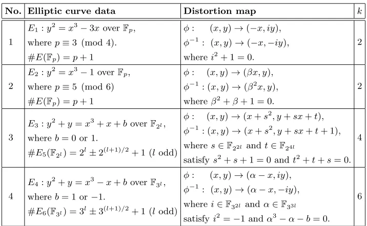
In practical implementations, the self-pairinge(P, P) can be designed byT ype1 pairings [11], i.e., it can be constructed on supersingular elliptic curves with even embedding degrees. For interests, we cite all cases as Table 1. Note that the computation of the pairings onE1 and E2 has been discussed [18]. In the
mean time, TheηT pairing can be defined onE3andE4[3]. Since the distortion
mapφ[26] is an isogeny, we list its dual isogenyφ−1 for convenience.
In this section, we will explore the computation of the self-pairings on the curves given in Table 1. Our general understanding of the construction of the self-pairings comes mostly from the following theorem.
Theorem 1. Let E be the supersingular curves over the ground field Fq given
in Table 1. Let r be a large prime dividing the order ofE(Fq). The embedding
degree with respect toris equal tok. Letπq be the Frobenius endomorphism and
take P ∈G1=Ker(πq−[1])∩E[r]. The self-pairing based on the Weil pairing
can be given by
es(P, P),eˆ(P, φ(P))2(q k/2
−1)=f
r,P(φ(P))4(q k/2
−1).
Proof. It follows from the definition of the Weil pairing that
es(P, P),eˆ(P, φ(P))2(q k/2
−1)= (fr,P(φ(P))
fr,φ(P)(P)
)2(qk/2−1).
Since the distortion map in Table 1 is an automorphism, we have
fr,φ(P)(P)(q
k/2
−1)=f
r,P(φ−1(P))(q k/2
Table 1.Popular pairing-friendly curves with distortion maps
No. Elliptic curve data Distortion map k
1
E1:y2=x3−3xoverFp, wherep≡3 (mod 4). #E(Fp) =p+ 1
φ: (x, y)→(−x, iy),
φ−1: (x, y)→(−x,−iy),
wherei2+ 1 = 0.
2
2
E2:y2=x3−1 overFp, wherep≡5 (mod 6) #E(Fp) =p+ 1
φ: (x, y)→(βx, y),
φ−1: (x, y)→(β2x, y),
whereβ2+β+ 1 = 0.
2
3
E3:y2+y=x3+x+boverF2l,
whereb= 0 or 1.
#E5(F2l) = 2l±2(l+1)/2+ 1 (lodd)
φ: (x, y)→(x+s2, y+sx+t),
φ−1: (x, y)→(x+s2, y+sx+t+ 1),
wheres∈F22l andt∈F24l
satisfys2+s+ 1 = 0 andt2+t+s= 0. 4
4
E4:y2+y=x3−x+boverF3l,
whereb= 1 or−1.
#E6(F3l) = 3l±3(l+1)/2+ 1 (lodd)
φ: (x, y)→(α−x, iy),
φ−1: (x, y)→(α−x,−iy),
wherei∈F32l andα∈F33l
satisfyi2=−1 andα3−α−b= 0. 6
which has been discussed in Proposition 2 of the paper [21]. Now it suffices to demonstrate that
( 1
fr,P(φ−1(P)))
(qk/2
−1)=f
r,P(φ(P))(q k/2
−1),
i.e.
(fr,P(φ−1(P))fr,P(φ(P)))(q k/2
−1)= 1. (1)
LetP = (xP, yP)∈G1. We will show that the equality (1) holds in the following.
Case 1. We first consider the curve E1. Let q=p, where p≡3 (mod 4). The
rational function fr,P can be written asa(x) +b(x)y, wherea(x) and b(x) are
the rational functions over the finite fieldFq in terms ofx[10]. We have
fr,P(φ−1(P)) =a(−xP)−b(−xP)yPi
and
fr,P(φ(P)) =a(−xP) +b(−xP)yPi.
It follows from Fermat’s little Theorem andi2+ 1 = 0 that
(fr,P(φ−1(P))fr,P(φ(P)))(q k/2
Case 2. Now we consider the curveE2. Letq=p, wherep≡2 (mod 3). Similar
to Case 1, the rational function fr,P can be written as c(y) +d(y)x+e(y)x2,
where c(y), d(y) and e(y) are the rational functions over the finite field Fq in
terms ofy. Applyingβ2+β+ 1 = 0, we get
fr,P(φ−1(P)) =c(yP) +d(yP)xPβ+e(yP)x2Pβ2
=(c(yP)−e(yP)x2P) + (d(yP)xP −e(yP)x2P)β
and
fr,P(φ(P)) =c(yP) +d(yP)xPβ2+e(yP)x2Pβ4
=(c(yP)−d(yP)xP) + (e(yP)x2P −d(yP)xP)β
=(c(yP)−e(yP)x2P)−(d(yP)xP −e(yP)x2P)(β+ 1).
It follows from Fermat’s little Theorem andβ2+β+ 1 = 0 that
(fr,P(φ−1(P))fr,P(φ(P)))(q k/2
−1)= 1.
Case 3. Now we consider the curve E3. Let q = 2l. Similar to the above, the
rational function fr,P can be written asa(x) +b(x)y, wherea(x) and b(x) are
the rational functions over the finite fieldFq in terms ofx. For convenience, we
use the notation aandb fora(xP+s2) andb(xP +s2), respectively. Then
fr,P(φ−1(P)) =a+b(yP+sxP+t+ 1)
=(a+byP+bsxP) +b(t+ 1)
and
fr,P(φ(P)) =a+b(yP +sxP+t)
=(a+byP +bsxP) +bt.
Sinces∈Fqk/2 andt2+t=s, it follows from Fermat’s little Theorem that
(fr,P(φ−1(P))fr,P(φ(P)))(q k/2
−1)= 1.
Case 4. Now we consider the curve E4. Letq= 3l. The rational function fr,P
can be written as a(x) +b(x)y, where a(x) andb(x) are the rational functions over the finite fieldFq in terms ofx. For convenience, we use the notationaand
bfora(α−xP) andb(α−xP), respectively. Then
and
fr,P(φ(P)) =a−byPi.
It follows from Fermat’s little Theorem that
(fr,P(φ−1(P))fr,P(φ(P)))(q k/2
−1)= 1.
Therefore the equality (1) holds in all cases. This completes the whole proof. We call our new pairing in Theorem 1 the Ateil pairing. In the case of the supersingular curves with embedding degree k= 2, we see that at any security level the Ateil pairing is faster than the self-pairing based on the reduce Tate pairing since the final exponentiation of the former is simpler than that of the latter and both of them have the same Miller loop. However, in the case of the supersingular curves with embedding degree k = 4 or 6, the self-pairing based on the ηT pairing whose Miller loop is half the length of that required for the
reduced Tate pairing. This leads to the proposed pairing in Theorem 1 is slower than the self-pairing based on the ηT pairing in this case. We next provide the
improvement of the Ateil pairing, as compared to the self-pairing based on the
ηT pairing.
3.1 An Improvement on the ηT Pairing
Our goal is to construct a new self-pairing which has the same Miller loop as the
ηT pairing. It is known that theηT pairing is the fastest pairing on supersingular
elliptic curves over finite fields with small characteristics 2 or 3 and Hess et. al
give another approach for the ηT pairing in Section 3.2 of [13]. We will mainly
consider the self-pairing computation in this case. The following lemma is useful for generating the Ateil pairing on supersingular elliptic curves over finite fields with small characteristics.
Lemma 1. Let E be the supersingular curves defined as Theorem 1. Letr be a
large prime satisfying r | #E(Fq) and denote the trace of the Frobenius
endo-morphism with t, i.e., #E(Fq) =q+ 1−t. The embedding degree with respect
to r is equal to k. Write T = t −1. For Ti = (t −1)i ≡ qi mod r where
1 ≤i≤k−1, we denote Ti =Ti mod r. Let abe the smallest positive integer
such thatTa
i ≡1 modr. There exists an integerLsuch thatTia−1 =Lr. Given
ˆ
e(P, φ(Q))2(qk/2−1)L= fTi,P(φ(Q))
fTi,Q(φ−1(P))
2(qk/2
−1)c
,
wherec=Pa−1
j=0T
a−1−j
i qej≡aqei(a−1) (mod r).
Proof. It is obvious from the definition of the Weil pairing and fr,φ(Q)(P) =
fr,Q(φ−1(P)) (see Proposition 2 of [21]) that
ˆ
e(P, φ(Q))2(qk/2−1)L= (fr,P(φ(Q))
fr,φ(Q)(P)
)2L(qk/2−1)= ( fLr,P(φ(Q))
fLr,Q(φ−1(P)))
2(qk/2
−1).
Applying the identityLr=Ta
i −1 into the above equation, we obtain
ˆ
e(P, φ(Q))2(qk/2−1)L= ( fT
a
i−1,P(φ(Q))
fTa
i−1,Q(φ−
1(P))) 2(qk/2
−1)= ( fT
a
i,P(φ(Q))
fTa i,Q(φ−
1(P))) 2(qk/2
−1)
(1) Since (ˆπq ◦π)(P) = [q]P = [T]P, we have ˆπqi(P) = [Ti]P = [Ti]P. Due to the
discussion in Section 3.2 of [13] (or see the proof of Theorem 1 in [3]), we see that
fTa
i,P(φ(Q)) = (fTi,P(φ(Q)))
Pa−1
j=0T (a−1−j)
i q
j
(2) Using the same argument forfTa
i,Q(φ
−1(P)), we have
fTa i,Q(φ
−1(P)) = (f
Ti,Q(φ−
1(P)))Pa−1
j=0T (a−1−j)
i qj. (3)
Substituting (2) and (3) into the equation (1), we have ˆ
e(P, Q)2(qk/2−1)L = ( fTi,P(φ(Q))
fTi,Q(φ−1(P))
)2(qk/2−1)c,
wherec=Pa−1
j=0T
a−1−j
i qj≡aqi(a−1) (modr). This completes the whole proof.
On the basis of Lemma 1, we can define a new powered pairing as ( fTi,P(φ(Q)) fTi,Q(φ−1(P)))
2(qk/2
−1) which will be non-degenerate provided thatr∤L. It has the same loop length as
theηT pairing wheni= 1. Despite this new pairing has the simple
exponentia-tion, it is slower than the ηT pairing since it involves two Miller iteration loops.
ApplyingQ=P in the new defined pairing ( fTi,P(φ(Q)) fTi,Q(φ−1(P)))
2(qk/2
−1), we have the following results.
Theorem 2. Using the same notation as above, the self-pairing based on theηT
pairing can be given by
es(P, P),(
fTi,P(φ(P))
fTi,P(φ−1(P))
)2(qk/2−1)=f
Ti,P(φ(P))
Proof. It is immediate from the proof of Theorem 1 and Lemma 1.
We call our new pairing in Theorem 2 the Ateili pairing. Some remarks on
the Ateili pairing are stated as follows.
Remark 1. A series of the Ateili pairing can be obtained as i varies. We call
the Ateilipairing with the shortest Miller loop is optimal. Due to the discussion
in [25, 12], the optimal Ateilipairing has the same loop length as theηT pairing.
Remark 2. The loop length of the Ateili pairing is as same as that of the ηT
pairing when i = 1. For Ti < 0, the generalized version of the Ateil pairing
suggests to useTi·(Ti)k/2=Ti·(−1) (modr) provided thatk >2.
Remark 3. At any security level, the optimal Ateili pairing will be faster than
the self-pairing based on the ηT pairing since the former has a simpler final
exponentiation than the latter and both of them have the same Miller loop.
Remark 4. The optimal Ateilipairing on supersingular elliptic curves over finite
fields with characteristic three can achieves better performance when imple-menting ZSS short signatures [28].
4
Self-pairing on Elliptic Curves with Embedding Degree
one
Since the distortion maps exist on not only supersingular elliptic curves but also ordinary elliptic curves with embedding degreeone, we will consider self-pairing computation on the latter curves in this section. Koblitz and Menezes first gave the concrete construction of ordinary curves with embedding degree one and analyzed the efficiency of pairing computations on these curves [18].
Assume that the primep=A2+ 1. The equation of the elliptic curveE 5over
Fp is defined by
E5:y2=x3+ax,
where a=−1 or−4. The order of the groupE5(Fp) is #E5(Fp) =p−1. Note
that the distortion map onE5is given byφ: (x, y)→(−x, Ay). In the following,
4.1 Self-pairing Based on the Weil pairing
It is known that the denominator elimination techniques can be used for speeding up the reduced Tate pairing [4] and the powered Weil pairing [18, 17] due to the final exponentiation. However, these methods can not be applied in the case of pairing computations on the curveE5with embedding degreeone. To apply the
denominator elimination techniques in self-pairing computations, we will define a new fixed power of the Weil pairing. LetP ∈E5(Fp) have prime orderr. The
self-pairing based on the Weil pairing can be defined as
es(P, P) = ˆe(P, φ(P))4. (4)
The following lemma shows that the proposed self-pairing (4) can be com-puted efficiently.
Lemma 2. The denominator elimination technique can be applied when
com-puting the self-pairing (4) on the curve E5 with embedding degree one.
Proof. In the case of the doubling steps of the self-pairings, after initially setting
T =P,f1=f2= 1, for each bit ofrwe do
T←2T f1←f12
lT,T(φ(P))
v2T(φ(P))
f2←f22
lφ(T),φ(T)(P)
vφ(2T)(P)
Assume thatP = (xP, yP) and 2T = (x2T, y2T). We obtainφ(P) = (−xP, AyP)
andφ(2T) = (−x2T, Ay2T). It is easy to check that
v2T(φ(P)) =−xP −x2T
vφ(2T)(P) =x2T −xP = (−1)·v2T(φ(P)).
Note that we can ignore−1 due to the final power f our. Thus the denomina-tors in the doubling steps can be eliminated. Similarly, it can be seen that the denominators in the addition steps can be also eliminated. This completes the proof of Lemma 2.
Doubling Step Assume thatT= (xT, yT), [2]T = (x2T, y2T) andP = (xP, yP).
LetlT,T be the equation of the tangent line through the point T andλbe the
slope of the line. We have
lT,T(φ(P)) = (AyP−yT)−λ(−xP −xT) = (−yT+λ(xP+xT)) +yP·A.
Observe that if the slope of the tangent line through the pointT is λ, then the slope of the tangent line through the pointφ(T) is−Aλ. It follows that
lφ(T),φ(T)(P) =yP−AyT+Aλ(xP +xT).
Then
(−A)lφ(T),φ(P)(P) = (−yT +λ(xP +xT))−yPA.
SinceA4= 1 (modp) and the final power equalsf our, we can replacel
φ(T),φ(T)(P))
by (−Alφ(T),φ(T)(P)) in the whole computation.
Note that we can cacheR1=A·yP. The formulas for the doubling steps in
affine coordinates will be given by
λ=3x
2
T+a
2yT
; x2T =λ2−2xT; y2T =λ·(xT−x2T)−yT
t1=−yT+λ·(xP+xT), t2=R1, f1←f12·(t1+t2), f2←f22·(t1−t2)
The total cost of the operation for the doubling steps in affine coordinates will be 1I+5M+4S, where I, M and S denote the costs of inversion, multiplication and squaring in the ground fieldFp.
Now we consider the operation count for the doubling steps in Jacobian coordinates. A point (X, Y, Z, W = Z2) in the modified Jacobian coordinates
corresponds to the point (x, y) in affine coordinates with x=X/Z2, y=Y /Z3.
Let T = (XT, YT, ZT, WT = ZT2) and N = 2T = (XN, YN, ZN, WN = ZN2).
Based on the explicit-formulas database given by Bernstein and Lange [5], the following formulas compute a doubling in 6M + 10S.
B=XT2;C=YT2;D=C2;E=WT2;S= 2((XT+C)2−B−D);M = 3B+aE;
XN =M2−2S;YN =M·(S−XN)−8D;ZN = (YT+ZT)2−C−WT;
wN =ZN2;t1=ZN ·WT ·R1;t2=−2C+M ·(WT ·xP+XT);
Addition Step Assume that T = (xT, yT), P = (xP, yP) andN =T +P =
(xN, yN). LetlT,P be the equation of the line through pointsT and P. Denote
byλthe slope of the linelT,P. We have
lT,P(φ(P)) = (AyP−yP)−λ(−xP−xP) = (−yP+ 2λxP) +yP·A.
Observe that if the slope of the line through pointsT andP isλ, then the slope of the line through points φ(T) andφ(P) is−Aλ. It follows that
lφ(T),φ(P)(P)) = (yP−AyP)−(−Aλ)(xP −(−xP)) =A(−yP+ 2λxP) +yP.
Then
(−A)lφ(T),φ(P)(P) = (−yP + 2λxP)−yP·A.
SinceA4= 1 (modp) and the final power equalsf our, it follows thatl
φ(T),φ(P)(P))
can be replaced by (−Alφ(T),φ(P)(P)) in the whole computation.
Similar to the doubling step, we can cacheR1=A·yP. The formulas for the
addition steps in affine coordinates can be given by
λ=yT−yP
xT−xP
; xN =λ2−xP −xT; yN =λ·(xP −xN)−yP;
t1=−yP+ 2λ·xP; t2=R1, f1←f1·(t1+t2), f2←f2·(t1−t2)
The total cost of the operation for the addition steps in affine coordinates will be 1I+5M+1S.
Now we consider the operation count for the addition steps in Jacobian co-ordinates. Note that we will cache R1 =A·yP, R3 = yP2, and R4 =x2P. Let
T = (XT, YT, ZT, WT =ZT2) andN = (XN, YN, ZN, WN =ZN2) =T+P. Based
on the explicit-formulas database given by Bernstein and Lange [5], the following formulas compute an addition step in 9M+ 7S.
U2=xP·WT;S2= (yP)·ZT ·WT;H=U2−XT;HH=H2;I= 4HH;
J =H·I;M =S2−YT;R= 2M;V =XT ·I;R2=R2;XN =R2−J−2V;
YN =R·(V−XN)−2YT·J;ZN = (ZT +H)2−WT−HH;WN =ZN2;
t1=(ZN +R1)2−WN+R3;t2=(ZN +yP)2−WN−R3+2((R+xP)2−R2−R4);
l1=t1+t2; l2=t1−t2; f1=f1·l1; f2=f2·l2;
4.2 Self-pairing Based on the Tate Pairing
the divisor D equals to (φ(P) +R)−(R). The self-pairing based on the Tate pairing is given by
es(P, P) = ¯e(P, φ(P)) = (
fr,P(φ(P) +R)
fr,P(R)
)(p−1)/r. (5)
Note that we can not replace the divisorDby the pointφ(P) for computing the reduced Tate pairing ¯e(P, φ(P)). We next analyze the cost of the doubling and addition steps for computing ¯e(P, φ(P)) in detail.
Doubling Step Let T = (xT, yT) and 2T = (x2T, y2T) in affine coordinate
systems. The functionlT,T andv2T correspond respectively, to the tangent line
to the curveE5 at the point T and the vertical line through the point 2T. For
each bit ofrwe do
λ=3x
2
T+a
2yT
; x2T =λ2−2xT; y2T =λ·(xT−x2T)−yT
f1←f12·lT,T(φ(P) +R)·v2T(R); f2←f22·lT,T(R)·v2T(φ(P) +R).
The formulas need 1I+8M+4S to compute the doubling step in affine coor-dinates. Koblitz and Menezes have considered the doubling steps which cost 13M+9S in Jacobian coordinates [18]. Ionica and Joux have given the improved formulas for the doubling steps in this case which cost 10M+10S [14].
Addition Step Assume that T = (xT, yT), P = (xP, yP) andN =T +P =
(xN, yN). The formulas for the addition steps will be given by
λ=yT −yP
xT −xP
; xN =λ2−xP −xT; yN =λ·(xP−xN)−yP;
f1←f1·lT,P(φ(P) +R)·vT+P(R); f2←f2·lT,P(R)·vT+P(φ(P) +R).
The total cost of the operation for the addition steps in affine coordinates will be 1I+8M+1S. Ionica and Joux have developed the improved formulas for the addition steps in Jacobian coordinates which cost 18M+3S [14].
4.3 Efficiency Consideration for Self-pairing on the Curve with
Embedding Degree one
In this subsection, we compare the efficiency of computing the self-pairings with different structures on the curveE5. We first note that the presented
which leads to the reduction of the computational complexity. Furthermore, we summarize the computational costs of basic doubling and addition steps for dif-ferent pairings into Table 2.
Table 2. Comparison of Basic Steps for Different Self-pairings on Curves with Em-bedding Degreesone
Coordinate System Self-pairings Doubling Steps Addition Steps
Affine coordinate Proposed pairing (4) 1I+5M+4S 1I+5M+1S Tate pairing (5) 1I+8M+4S 1I+8M+1S Jacobian coordinate Proposed pairing (4) 6M+10S 9M+7S
Tate pairing (5) 10M+10S 18M+3S
As shown in Table 2, computing the proposed self-pairing (4) needs fewer multiplications than computing the reduced Tate pairing (5) on the curve E5
with embedding degree one in each step. We conclude that the proposed self-pairing (4) is faster than the self-self-pairing (5) based on the Tate self-pairing at any security level.
5
Conclusion
In this paper, the computation of the self-pairing is considered in all cases. Using the symmetry of the structure of the Weil pairing, we have presented the Ateil pairing withoneMiller loop. The proposed pairings achieve better performance than the previously known self-pairings at any security level. From the Ateil pairing approach, we see that the variant of the Weil pairing may be preferred in certain cases.
References
1. C. Arene, T. Lange, M. Naehrig and C. Ritzenthaler. “Faster Computation of the Tate Pairing,” Preprint, 2009. Available from http://eprint.iacr.org/2009/155. 2. R. Avanzi, H. Cohen, C. Doche, G. Frey, T. Lange, K. Nguyen, and F. Vercauteren.
3. P.S.L.M. Barreto, S. Galbraith, C. ´Oh´Eigeartaigh, and M. Scott. “Efficient pairing computation on supersingular Abelian varieties,” Designs, Codes and Cryptogra-phy, vol. 42, no. 3. Springer Netherlands, 2007.
4. P.S.L.M. Barreto, H.Y. Kim, B. Lynn, and M. Scott. “Efficient algorithms for pairing-based cryptosystems,” Advances in Cryptology-Crypto’2002, volume 2442 ofLecture Notes in Computer Science, pp. 354-368. Springer-Verlag, 2002. 5. D. J. Bernstein and T. Lange. Explicit-formulas database.
http://www.hyperelliptic.org/EFD
6. C. Costello, T. Lange, and M. Naehrig. “Faster Pairing Computations on Curves with High-Degree Twists,” Public Key Cryptography - PKC 2010, Volume 6056 ofLecture Notes in Computer Science, pp. 224-242, Springer-Verlag, 2010. 7. I. Duursma, H.-S. Lee. “Tate pairing implementation for hyperelliptic curvesy2=
xp−x+d,”Advances in Cryptology-Asiacrypt’2003, volume 2894 ofLecture Notes in Computer Science, pp. 111-123. Springer-Verlag, 2003.
8. G. Frey and H-G. R¨uck. “A remark concerning m-divisibility and the discrete logartihm in the divisor class group of curves,”Math. Comp.,vol. 62(206), pp.865-874, 1994.
9. S. Galbraith. Pairings. Chapter IX of In: I. Blake, G. Seroussi, N. Smart(eds) Advances in Elliptic Curve Cryptography. Cambridge University Press, 2005. 10. S. D. Galbraith, F. Hess, and F. Vercauteren. “Aspects of Pairing Inversion,”IEEE
Trans. Inform. Theory vol.54, No. 12, pp. 5719-5728, 2008.
11. S.D. Galbraith, K. Paterson, N. Smart. “Pairings for cryptographers,”Discr. Appl. Math.vol. 156, pp. 3113-3121, 2008.
12. F. Hess. “Pairing lattices,” Pairing 2008,Volume 5209 ofLecture Notes in Com-puter Science,pp. 18-38, Springer-Verlag, 2008.
13. F. Hess, N.P. Smart and F. Vercauteren. “The Eta pairing revisited,”IEEE Trans. Infor. Theory, vol 52, pp. 4595-4602, Oct. 2006.
14. S. Ionica and A. Joux. “Another approach to pairing computation in Edwards coordinates,” IndoCrypt 2008, Volume 5365 ofLecture Notes in Computer Science, pp. 400-413, 2008.
15. E. Lee, H.-S. Lee, and C.-M. Park. “Efficient and generalized pairing computation on Abelian varieties,”IEEE Trans. Inform. Theory, vol. 55, no.4, pp. 1793-1803, 2009.
16. S. Matsuda, N. Kanayama, F. Hess, and E. Okamoto. “Optimised versions of the Ate and twisted Ate pairings,”The 11th IMA International Conference on Cryp-tography and Coding, Volume 4887 of Lecture Notes in Computer Science, pp. 302-312. Springer-Verlag, 2007.
18. N. Koblitz, and A. J. Menezes. “Pairing-based cryptography at high security lev-els,”Cryptography and Coding, Volume 3796 ofLecture Notes in Computer Science, pp. 13-36. Springer-Verlag, 2005.
19. V.S. Miller. “Short programs for functions on curves,” Unpublished manuscript, 1986. Available from http://crypto.stanford.edu/miller/miller.pdf.
20. V.S. Miller. “The Weil pairing and its efficient calculation,” J. Cryptology, vol. 17, no. 44, pp. 235-261, 2004.
21. C. M. Park, M. H. Kim, and M. Yung. “A Remark on Implementing the Weil Pairing,” CISC 2005, Volume 3822 of Lecture Notes in Computer Science, pp. 313-323, 2005.
22. K. G. Paterson, “ID-based signatures from pairings on elliptic curves,” Electronics Letters, vol. 38, No. 18, pp. 1025-1026, 2002.
23. K.G. Paterson. Cryptography from Pairing - Advances in Elliptic Curve Cryptog-raphy. Cambridge University Press, 2005.
24. M. Scott, N. Benger, M. Charlemagne, L. J. Dominguez Perez, and E. J. Kachisa. “On the Final Exponentiation for Calculating Pairings on Ordinary Elliptic Curves,” Pairing 2009, Volume 5671 of Lecture Notes in Computer Science, pp. 78-88, 2009.
25. F. Vercauteren. “Optimal pairings,” IEEE Trans. Inform. Theory,vol. 56, no.1, pp. 455-461, 2009.
26. E. Verheul, “Evidence that XTR is more secure than supersingular elliptic curve cryptosystems,”Advances in Cryptology - Eurocrypt 2001, Volume 2045 ofLecture Notes in Computer Science, pp. 195-210, Springer-Verlag, 2001.
27. F. Zhang, X. Chen, W. Susilo and Y. Mu. “A New Signature Scheme Without Random Oracles from Bilinear Pairings,”VietCrypt 2006, Volume 4341 ofLecture Notes in Computer Science, pp.67-80, Springer-Verlag, 2006.
28. F. Zhang, R. Safavi-Naini and W. Susilo, “An efficient signature scheme from bilinear pairings and its applications,” PKC 2004, Volume 2947 ofLecture Notes in Computer Science, pp.277-290, Springer-Verlag, 2004.
29. F. Zhang, R. Safavi-Naini, W. Susilo, “ID-Based Chameleon Hashes from Bilinear Pairings,” Cryptology ePrint Archive, Report 2003/208.
30. C.-A. Zhao, D.Q. Xie, F. Zhang, J. Zhang and B.-L. Chen. “Computing Bilinear Pairings on Elliptic Curves with Automorphisms,”Designs, Codes and Cryptogra-phy, To appear.
31. C.-A. Zhao, F. Zhang and J. Huang. “A note on the Ate pairing,” Int. J. Inf. Security, vol. 7, no. 6, pp. 379-382, 2008.