On isogeny classes of Edwards curves over finite fields
Omran Ahmadi Robert Granger
omran.ahmadi@ucd.ie rgranger@computing.dcu.ie Claude Shannon Institute
University College Dublin Dublin 4
Ireland March 17, 2011
Abstract
We count the number of isogeny classes of Edwards curves over finite fields, answering a question recently posed by Rezaeian and Shparlinski. We also show that each isogeny class contains acomplete Edwards curve, and that an Edwards curve is isogenous to anoriginal Edwards curve over IFq if and only
if its group order is divisible by 8 ifq≡ −1 (mod 4), and 16 ifq≡1 (mod 4). Furthermore, we give formulae for the proportion ofd∈IFq\ {0,1} for which
the Edwards curveEd is complete or original, relative to the total number ofd
in each isogeny class.
1
Introduction
In 2007 Edwards proposed a new normal form for elliptic curves over a field k of characteristic 6= 2 [6], namely:
Ea(k) :x2+y2 =a2(1 +x2y2), (1)
for a5 6= a. Bernstein and Lange generalised Edwards’ form to incorporate curves of the form
E(k) :x2+y2 =a2(1 +dx2y2),
which is elliptic if ad(1−da4) 6= 0 [3]. All curves in the Bernstein-Lange form are isomorphic to curves of the following form, referred to as Edwards curves:
Ed(k) :x2+y2= 1 +dx2y2. (2)
attacks [4, Chapters 4 and 5];completewhendis a non-square, which means the ad-dition formulae work for all input points; and are the most efficient in the literature. Bernstein et al. have also considered twistedEdwards curves [2]:
Ea,d(k) :ax2+y2 = 1 +dx2y2, (3)
which includes more curves over finite fields than does Edwards curves.
Rezaeian and Shparlinski have computed the exact number of distinct curves of the form (1) and (2) over a finite field IFq of characteristic>2, up to isomorphism
over the algebraic closure of IFq [7]. However they state that counting the number
of distinct isogeny classes over IFq for these curves is a very natural and challenging
question.
In this paper we answer this question fully for fields of characteristic >2. Our starting point is interesting in that it was serendipitous, beginning with an incidental empirical observation. When searching for suitable parameters for elliptic curve cryptography, for curves of the form (2), we observed that over a finite field IFp with p≡1 (mod 4), it (empirically) holds that
#Ed(IFp) = #E1−d(IFp),
and hence by Tate’s theorem [16], Ed and E1−d should be isogenous over IFp.
In the course of proving the above observation using character sum identities, we discovered that the Edwards curveEd is isogenous to the Legendre curve:
Ld(Fq) :y2 =x(x−1)(x−d). (4)
With explicit computation one sees that this isogeny has degree two, and so Ed
inherits a set of 4-isogenies from the well-known set of isomorphisms ofLd, each as
the composition of the 2-isogeny to Ld, an isomorphism of Ld toLd0, and the dual
of the 2-isogeny from Ed0 to Ld0. In particular Ed/IFp is 4-isogenous to E1−d/IFp
for p ≡ 1 (mod 4). More generally, for Ed over any finite field IFq one obtains
4-isogenies toE1−d,E1/d,E1−1/d,E1/(1−d)andEd/(d−1), being defined over IFqor IFq2
depending on the quadratic character of −1, dand 1−din IFq.
We later learned that the above 2-isogeny is merely a special case of Theorem 5.1 of [2], which states that any elliptic curve with three IFq-rational 2-torsion points
is 2-isogenous to a twisted Edwards curve of the form (3). However the explicit connection with the Legendre curve and the consequent ramifications contained herein has — to the best of our knowledge — not been made before.
relative to the total number of din each isogeny class. This total be computed via a Deuring-style class number formula derived by Katz [11], and hence for a given trace one can compute the number of complete Edwards curve parametersd.
We also address the distribution of original Edwards curves (1) amongst the isogeny classes of Edwards curves. Forq ≡ −1 (mod 4) this follows from our result on complete Edwards curves, but for q ≡ 1 (mod 4) we express the proportion of such curves in a given isogeny class using a set of remarkable ratio results due to Katz [11]. Whilst we believe our results may be proven succinctly using a variation of Katz’s approach, our arguments for the proportion of complete and original Edwards curves rely only on explicit bijections between sets of curves of different parameter types, and are thus entirely elementary.
Notation: For two elliptic curves over a fieldk, we writeE ∼E0whenEis isogenous toE0 overk, and E =∼E0 when E is isomorphic to E0 over the algebraic closure of
k. Throughout the paper, IFp refers to a finite field of prime cardinalitypand IFqto
an extension field of cardinalityq =pm, where m≥1. Also, if the field of definition of a curve or map is not specified, it is assumed to be a field of characteristic 6= 2.
2
A point counting proof of
E
d(
F
q)
∼
L
d(
F
q)
It is well known that the elliptic integral
Z p(x)
p
q(x)dx,
where p(x)∈ IR(x) is a rational function andq(x)∈IR[x] is a quartic polynomial, can be reduced to
Z
p1(x) p
q1(x) dx
for a rational function p1(x)∈IR(x) and a cubic polynomial q1(x)∈IR[x] provided
that one knows one of the roots of q(x) [19, Chapter 8].
The finite field analogue of this fact is the following result of Williams [21].
Lemma 2.1. [21] Let q be an odd prime power and let IFq denote the finite field
withq elements. Suppose thatF(x) is a complex valued function from IFq to Cand
also let χ2(·) denote the quadratic character of IFq. Also let Z denote the zero set
of a2x2+b2x+c2. Then
X
x∈IFq\Z
F
a1x2+b1x+c1 a2x2+b2x+c2
= X
x∈IFq
χ2(Dx2+ ∆x+d)F(x) (5)
+ X
x∈IFq
F(x)−
F
a1 a2
, if a2 6= 0,
where a1, b1, c1, a2, b2, c2∈IFq,
D=b22−4a2c2, ∆ = 4a1c2−2b1b2+ 4a2c1, d=b21−4a1c1, (6)
and
∆2−4dD6= 0.
In the following we use the lemma above to show that Ed(Fq) is isogenous to Ld(Fq). First notice that the given singular model for Edwards curves (2) has two
points at infinity which are singular and no affine singular points, and resolving the singularities results in four points which are defined over Fq if and only if d is a
quadratic residue in Fq [3]. Thus the non-singular model ofEd(Fq) has 2 + 2χ2(d)
points more than the singular model of Ed(Fq), and hence if we rewrite the curve
equation ofEdas
Ed(Fq) :y2 = x 2−1
dx2−1, (7)
then
#Ed(Fq) = 2 + 2χ2(d) +
X
x∈IFq, x6=±d1/2
(1 +χ2
x2−1 dx2−1
)
= 2 + 2χ2(d) +q−(1 +χ2(d)) +
X
x∈IFq, x6=±d1/2
χ2
x2−1
dx2−1
= q+ 1 +χ2(d) +
X
x∈IFq, x6=±d1/2
χ2
x2−1
dx2−1
. (8)
Now on the one hand by applying Lemma 2.1 with F(x) =χ2(x), we get
X
x∈IFq, x6=±d1/2
χ2
x2−1 dx2−1
= X
x∈IFq
χ2(4dx2−(4 + 4d)x+ 4)χ2(x)
+ X
x∈IFq
χ2(x)−χ2(d)
= X
x∈IFq
χ2((x−1)(dx−1))χ2(x)−χ2(d)
= X
x∈IFq
χ2(x(x−1)(x−d))−χ2(d), (9)
and on the other hand we have
#Ld(Fq) =q+ 1 + X
x∈IFq
χ2(x(x−1)(x−d)), (10)
where −P
x∈IFqχ2(x(1−x)(x−d)) is the trace of the Frobenius endomorphism.
Theorem 2.2. The Edwards curve Ed(Fq) and Legendre curve Ld(Fq) are
isoge-nous.
Lemma 2.1 can be viewed as a means of establishing isogeny relations between curves defined by relations such as
y2= a1x
2+b 1x+c1 a2x2+b2x+c2
, (11)
and curves defined by y2 = x(Dx2 + ∆x+d). In §8 we show how to derive an addition law for curves of the form (11) and prove results similar to those presented in the intervening sections.
3
4
-isogenies of
E
dIn this section we detail how to compute explicit 4-isogenies forEd, starting with the
2-isogeny fromEd toLdand its dual. We then detail the well-known isomorphisms
of Ld and compose these maps to form the desired 4-isogenies.
3.1 Explicit 2-isogeny ψd :Ed →Ld
We now derive a 2-isogeny from Ed toLd, as presented in the following result. Theorem 3.1. Let (x, y)∈Ed. Then ψd:Ed→Ld
(x, y)7→
1
x2,
y(d−1)
x(1−y2)
.
is a 2-isogeny. The dual of ψd is ψbd:Ld→Ed:
(x, y)7→
2y d−x2,
y2−x2(1−d)
y2+x2(1−d)
.
Note that ψd is defined on all points of Ed except the kernel elements (0,±1),
which map toO ∈Ld.
Proof. One has the following birational transformationτ
τ(x, y) =
(1−d)1 +y
1−y,(1−d)
2(1 +y)
x(1−y)
,
from Edto the Weierstrass curve
Wd:y2=x3+ 2(1 +d)x2+ (1−d)2x,
with inverse
τ−1(x, y) =
2x y ,
x−(1−d)
x+ (1−d)
While τ is not defined for the points (0,±1) ∈ Ed, one obtains an
everywhere-defined isomorphism between the respective desingularized projective models by sending (0,1) to O ∈ Wd and (0,−1) to (0,0). Similarly, τ−1 is not defined at
points (x, y) ∈Wd satisying y(x+ 1−d) = 0, but ifd is a square the points other
than (0,0) map to points of order 2 and 4 at infinity on the desingularisation ofEd
(see the discussion on exceptional points after Theorem 3.2 of [2]). The 2-isogeny used in the proof of Theorem 5.1 of [2] now maps Wd directly to Ldvia
φd(x, y) =
y2
4x2,
y((1−d)2−x2)
8x2
,
with dual
b
φd(x, y) =
y2 x2,
y(d−x2)
x2
.
One can verify that the compositions φd◦τ and τb◦φbd give the stated ψd and ψbd
respectively. ut
3.2 Isomorphisms of Ld
The set of isomorphisms ofLdare induced by the two involutionsσ1(d) = 1−dand σ2(d) = 1/d, which induce the following maps fromLdtoL1−dandL1/drespectively:
σ1: Ld−→L1−d: (x, y)7→(1−x,
√
−1y), (12)
σ2: Ld−→L1/d: (x, y)7→(x/d, y/d3/2). (13)
As transformations acting on a given field, the group generated byσ1, σ2 is: H={1, σ1, σ2, σ1σ2, σ2σ1, σ1σ2σ1},
which is isomorphic to the symmetric group S3. The orbit of d 6= 0,1 under the
action of H is
n
d,1−d,1 d,1−
1
d,
1 1−d,
d d−1
o
(14)
which has 6 distinct elements provided that d is not a root of d2 −d+ 1 = 0 or (d+ 1)(d−2)(2d−1) = 0. Hence we have isomorphisms between each pair of
Ld, L1−d, L1/d, L1−1/d, L1/(1−d) and Ld/(d−1). For completeness we give here the
remaining three isomorphisms fromLd toLσ(d) not listed in (12),(13):
σ1σ2: Ld−→L1−1
d : (x, y)
7→(1−x/d,√−1y/d3/2), (15)
σ2σ1: Ld−→L 1
1−d : (x, y)7→
1−x
1−d,
√ −1y
(1−d)3/2
, (16)
σ1σ2σ1 : Ld−→L d
d−1 : (x, y)
7→
x−d
1−d,− y
(1−d)3/2
3.3 4-isogenies of Ed to Eσ(d)
Letσ ∈H. Then ωσ(d):Ed→Eσ(d) is obtained as the following composition:
ωσ(d)=ψbσ(d)◦σ◦ψd.
The 2-isogeny ψbσ(d) can be obtained by taking ψbd and substituting σ(d) ford. We
do not write down all possible 4-isogenies but note that whether each is defined over IFq or IFq2 is dependent upon the quadratic character of −1, d and 1−d, as
determined by maps (12–17). For example, forq ≡1 (mod 4) one has χ2(−1) = 1
and so σ1 is defined over IFq and Ed ∼ E1−d, which was our original observation.
We note that the duals of each of these isogenies are also easily computed.
3.4 4-isogenies of twisted Edwards curves
One can also map twisted Edwards curves (3) to a Legendre form curve, as given by the following theorem, the proof of which is the same as the proof of Theorem 3.1, one having first applied the isomorphism Ea,d→Ed/a: (x, y)7→(
√
ax, y).
Theorem 3.2. Let (x, y)∈Ea,d. Then ψa,d:Ea,d→Ld/a:
(x, y)7→
1
ax2,
y(d−a)
a3/2x(1−y2)
.
The dual of ψa,d is ψba,d:Ld/a→Ea,d:
(x, y)7→
2√ay d−ax2,
ay2−x2(a−d) ay2+x2(a−d)
.
One therefore obtains a set of 4-isogenies from the isomorphisms ofLd/a, exactly as before.
4
Isomorphisms from
L
dto Edwards curves
In addition to the above 2-isogeny betweenEd and Ld, one can also consider when Ld is birationally equivalent to an Edwards curve, i.e., is isomorphic to an Edwards
curve. Such isomorphisms have two immediate consequences. Firstly, for each such isomorphism one obtains a 2-isogeny of Ed to another Edwards curve Ed0 via the
composition of ψd and the isomorphism, see §4.1. Secondly, one is able to deduce
4.1 Isomorphisms from Ld to Ed¯
SinceLd:y2 =x3−(1 +d)x2+dx, one can transform Ldto the Montgomery curve
MA,B :By2 =x3+Ax2+x
with A = −(1 +d)/√d, B = 1/d√d via (x, y) 7→ (x/√d, y). Using Theorem 3.2 of [2] one then obtains
x y√d,
x−√d x+√d
!
∈E−d(1−√
d)2,−d(1+√d)2,
which is isomorphic toEd¯with ¯d=
1+√d 1−√d
2
with
ρd:Ld→Ed¯: (x, y)7→
√
−1(1−√d)x
y,
x−√d x+√d
! .
Taking the negative root of d in the above transformations gives a second isomor-phism, which together we write as
ρd,±:Ld→Ed¯±1 : (x, y)7→
√
−1(1∓√d)x
y,
x∓√d x±√d
! .
We also have
b
ρd,±:Ed¯±1 →Ld: (x, y)7→
±√d1 +y
1−y,±
√ −1
√
d(1∓√d) 1 +y
x(1−y)
.
Clearly these isomorphisms are only defined over the ground field if both−1 andd
are quadratic residues.
Observe that the value ¯dis invariant under the substitutiond←1/d, hence the
Ld-isomorphic curveL1/dmaps toEd¯also, but with the±isogenies defined instead
by
ρ1/d,± :L1/d→Ed¯±1 : (x, y)7→
√
−1(1∓p1/d)x
y, x∓p
1/d x±p
1/d !
,
with inverseρb1/d,±:Ed¯±1 →L1/d:
(x, y)7→
±p1/d1 +y
1−y,±
√
−1p1/d(1∓p1/d) 1 +y
x(1−y)
.
Similarly, one can first map Ld toLσ(d) for anyσ ∈H, and then applyρd,±but
have twelve isomorphisms θσ(d),± from Ld to the six curves Ed¯±1 i for i
∈ {1,2,3}, with:
¯
d±11= 1±
√
d
1∓√d !2
,d¯±21=
1±√1−d
1∓√1−d 2
and ¯d±31 =
1±q d d−1
1∓q d d−1
2
.
As noted above the twelve isomorphisms have only the six image curvesEd¯±1 1 , Ed¯
±1 2
andEd¯±1
3 , sincedand 1/dmap to ¯d1, 1−dand 1/(1−d) map to ¯d2, andd/(d−1) and
1−1/d map to ¯d3. These curves are therefore isomorphic and each has j-invariant
28(d2−d+ 1)3 (d(d−1))2 ,
which is the Legendre curvej-invariantjL(d).
Taking the composition of ψd and an isomorphism from each of the six pairs of
isomorphisms above — one from each pair that have the same image — one obtains 2-isogenies ofEdtoEd¯±1
1 , Ed¯ ±1
2 andEd¯ ±1
3 , again defined over IFqor IFq
2 depending on
the quadratic charcter of−1, dand 1−d, which we summarise in Theorem 4.1. We note that Moody and Shumow have independently given equivalent isogenies [12], having obtained them using a different approach.
Theorem 4.1. There exist 2-isogenies of Ed to Ed¯±1 1 , Ed¯
±1
2 and Ed¯ ±1
3 , given by the
following maps, respectively:
(a) d1,¯ ±:Ed→Ed¯±1
1 : (x, y)7→ √−
1(1∓√d) d−1
1−y2 xy ,
1∓√dx2 1±√dx2
,
(b) d2,¯ ±:Ed→Ed¯±1
2 : (x, y)
7→(1∓√1−d)xy,1−(1∓
√
1−d)x2 1−(1±√1−d)x2
,
(c) d3,¯ ±:Ed→Ed¯±1
3 : (x, y)
7→ √
d−1∓√d 1−d
x y,
1− d±(1−d)
q
d d−1
x2 1− d∓(1−d)
q d d−1 x2 ! .
Theorem 4.1 allows one to write down the set of 4-isogenies betweenEdand any Eσ(d) via isogenies and isomorphisms of Edwards curves only: first mapEd→Ed¯±1
i ;
second apply an isomorphism to the relevant Ed¯±1
j ; and third use a dual isogeny
to map to Eσ(d). However, since the Edwards 2-isogenies implicitly depend on the
2-isogeny toLd, the initial derivation given is perhaps the most natural way to view
these 4-isogenies.
4.2 Isomorphisms of Ed
It is clear from§4.1 that theEd¯±1
i curves inherit isomorphisms from the isomorphisms
Ld plays a fundamental role. A natural question is whether or not it is possible to
exploit the isomorphisms between Ed¯±1
i to give the set of curves isomorphic toEd?
Since the j-invariant ofEd is [2]
jE(d) =
16(d2+ 14d+ 1)3
d(d−1)4 ,
it would not seem obvious how to determine the set of isomorphic curves ofEdfrom
those ofLd. However, one can argue as follows. As above letδ = ¯d1(d) =
1+√d 1−√d
2
,
with ¯d1 considered as a function of d. Observe that d= ( ¯d1(δ))−1, and hence Ed=E
1−√δ 1+√δ
2.
Since the curve on the right-hand-side is isomorphic toEd¯±1 1 (δ),Ed¯
±1
2 (δ) andEd¯ ±1 3 (δ),
so is Ed. Writing these expressions out in full gives the following theorem.
Theorem 4.2. Let Ed andEd0 be two Edwards curves. Then Ed∼=Ed0 if and only
if
d0 ∈
(
d,1/d, 1±d 1/4
1∓d1/4 !4
, 1±
√ −1d1/4
1∓√−1d1/4 !4)
.
These six values are naturally implied by Proposition 6.1 of Edwards original exposition [6]. In particular curve (1) is isomorphic to curve (2) via the map (x, y)7→
(ax, ay), with d = a4. Taking the fourth power of each of the 24 values given in Edwards’ proposition gives the six values listed in Theorem 4.2. It is however interesting that these values can be determined from the isomorphisms of Ldalone.
The above manipulations also show thatEd∼=Lδ, via
(x, y)7→ √
d+ 1
√
d−1 · 1 +y
1−y,
2√−1(1 +√d) (1−√d)2 ·
1 +y x(1−y)
! .
Note that the existence of such an isomorphism is implied by the fact thatjL(δ) = jE(d).
5
The number of isogeny classes of Edwards curves over
finite fields
In this section we derive some results about Edwards curves (2), from results known for the Legendre family of elliptic curves, which is well-studied. Having established the isogeny between Ed and Ld in Theorem 3.1, the validity of this approach is
immediate. In particular we determine the number of isogeny classes of Edwards curve over the finite field Fq, and in the course of doing so also detail the number
For the Legendre curve Ld(Fq), we denote the trace of the Frobenius
endomor-phism
− X
x∈IFq
η(x(x−1)(x−d)) (18)
by A(d,Fq). Then Equation (10) implies
#Ld(Fq) =q+ 1−A(d,Fq), (19)
and by the Hasse-Weil bound we have
|A(d,Fq)| ≤2
√
q.
Thus the number of isogeny classes of the Legendre family of elliptic curves is the same as the number of integer values of A with |A| ≤ 2√q for which there is a d
such that A(d,Fq) = A. The following two lemmata give a satisfactory answer to
this question. The first addresses the number of ordinary isogeny classes and the second addresses the supersingular isogeny classes.
Lemma 5.1. [11] LetFq be a finite field of odd characteristic, and letA∈ZZ be an
integer prime top (the characteristic of Fq) with |A| ≤2√q. If A≡q+ 1 (mod 4),
then there exists d∈Fq\{0,1} with A(d,Fq) =A.
Lemma 5.2. [11] Let p be an odd prime. Then we have the following assertions. (i) If q =p2k+1, and Ld(Fq) is supersingular, then A(d,Fq) = 0.
(ii) If q =p2k, and Ld(Fq) is supersingular, then A(d,Fq) =2pk, where =±1
is the choice of sign for which pk≡1 (mod 4).
Following Katz, we say that each A satisfying the conditions of Lemma 5.1 is
unobstructed, forq. From the two lemmata above, the following is immediate.
Corollary 5.3. Ifq=p2k+1 andp≡1 (mod 4), then the number of isogeny classes of Edwards curves over Fq is
2
b
2√qc+ 2 4
−2
jb2√qc p
k
+ 2
4
.
Proof. The claim will follow if we prove that there is no supersingular Legendre curve in this case. Observe that #Ld(Fq) is always divisible by 4, and ifq =p2k+1, p ≡ 1 (mod 4) and Ld(Fq) is supersingular, then from Lemma 5.2(i) and (19) it
In order to obtain the number of isogeny classes of Edwards curves in the re-maining cases we need to know how the supersingular Legendre curve parameters are distributed amongst extensions of the prime subfield IFp of IFq; again, there is
already a complete answer to this question in the literature. On the one hand, it is well known that Ld(Fq) is a supersinular curve if and only if d is a root of the
Hasse-Deuring polynomial
Hp(x) = (−1) p−1
2 p−1
2 X
i=0
(p−1)/2
i 2
xi,
and on the other hand it is well known that all the roots of Deuring polynomial are in IFp2 (see for example [1, Proposition 2.2]). Using Theorem 3.1 and [1,
Proposi-tion 3.2] the following is immediate.
Theorem 5.4. The number Sp of IFp-rational roots of the Deuring polynomial, or
equivalently the number of supersingular Edwards curves over IFp, satisfies
(i) Sp = 0 if and only if p≡1 (mod 4).
(ii) S3 = 1.
(iii) If p ≡ 3 (mod 4) and p > 3, then Sp = 3h(−p), where h(−p) is the class
number ofQ(
√ −p).
Corollary 5.5. Ifp≡3 (mod 4)andq =p2k+1, then the number of isogeny classes of Edwards curves over Fq is
2
b2√qc
4
−2
b2√qc
4p
+ 1.
Proof. From Lemma 5.2 and Theorem 5.4 it follows that there is a single isogeny class of supersingular Legendre curves in this case. ut
Similarly we have:
Corollary 5.6. If q =p2k for an odd prime p, then the number of isogeny classes of Edwards curves over Fq is
2
b2√qc+ 2
4
−2
jb2√qc p
k
+ 2
4
+ 1.
Proof. From the fact that all the roots of Hasse-Deuring polynomial are in Fp2
and from Lemma 5.2, it follows that there is a single isogeny class of supersingular
6
Isogeny classes of
complete
Edwards Curves
Bernstein and Lange proved that the Edwards addition law is complete, i.e., is well-defined on all inputs, if and only if χ2(d) =−1 [3]. A natural question to consider
is whether there exists a complete Edwards curve in every isogeny class. In this section we answer this question affirmatively, relating the number of non-square
d∈IFq\ {0,1}in each isogeny class to the total number ofdin each isogeny class.
6.1 Katz’s ratio results
While investigating the Lang-Trotter conjecture [10], Katz discovered some remark-able relationships between the number of d ∈ IFq \ {0,1} such that A(d,IFq) = q+ 1−#Ld =A for any unobstructedA, and the number of d∈IFq\ {0,1} such
thatA(d,IFq) =−A[11].
In particular, let N(A) = #{d ∈IFq\ {0,1}|A(d,IFq) =A}. Katz proved that
forq ≡ −1 (mod 4), one hasN(A) =N(−A). For q ≡1 (mod 4), this is no longer the case. SinceA≡2 (mod 4), exactly one of A,−Ahasq+ 1−A≡0 (mod 8) — call it A — with q+ 1 +A≡4 (mod 8). Then N(A)> N(−A). Furthermore, for
q ≡ 5 (mod 8) the ratior =N(A)/N(−A) is always one of the integers 2,3, or 5, depending only on the power of 2 dividing q+ 1−A, as given in:
Theorem 6.1. [11, Theorem 2.8] Supposeq ≡5 (mod 8). Then
ord2(q+ 1−A) = 3 =⇒r = 2, ord2(q+ 1−A) = 4 =⇒r = 3, ord2(q+ 1−A)≥5 =⇒r = 5.
For q ≡ 1 (mod 8) the situation is more complicated. If ord2(q+ 1−A) = 3
thenr = 2 as before. Let ∆ =A2−4q. For the remaining cases we have:
Theorem 6.2. [11, Theorem 2.11] Suppose q ≡1 (mod 8), and that ord2(q+ 1− A)≥4. Then ord2(∆)≥6, and we have the following results.
(1) Suppose ord2(∆) = 2k+ 1, k≥3. Then r= 5−3/2k−2.
(2) Suppose ord2(∆) = 2k, k≥3. Then
(a) if ∆/22k≡1 mod 8, then r= 5,
(b) if ∆/22k≡3 or 7 mod 8, then r= 5−3/2k−2,
(a) if ∆/22k≡5 mod 8, then r= 5−1/2k−3.
To explain these phenomena, Katz uses the fact that Ld is 2-isogenous to the
Katz derives a Deuring-style class number formula to express the number oft∈IFq
such that A(t,IFq) = A. Expressing the same for −A and then computing the
ratio N(A)/N(−A) happens to be far simpler than computing the exact numbers themselves, as it obviates the need to perform any class group order computations. However, in the proof no consideration was given (nor was it needed) of the quadratic character of elementstin a givenN(A). Furthermore, since under this 2-isogeny we havet= (1−d)/4, determining how the corresponding square and non-squaredare distributed between the numerator and denominator of N(A)/N(−A) is certainly not immediate.
However, we observed (empirically - and then proved) that the following holds. Let N2(A) and Nn2(A) be the partition of N(A) into square and non-squared
re-spectively, and similarly for−A. Forq ≡1 (mod 4), we haveNn2(A) =Nn2(−A) = N(−A), i.e., the smallest of the two valuesN(A), N(−A). Hence the excess ofN(A) overN(−A) consists entirely of square d. Forq ≡ −1 (mod 4) we have
Nn2(A) = (
N(A) ifq+ 1−A≡4 (mod 8)
N(A)/3 if q+ 1−A≡0 (mod 8).
Since q ≡ −1 (mod 4) we have Nn2(A) = Nn2(−A) in this case also. Our proof of
these facts is elementary.
6.2 Proof of claims
We use the following three lemmata, the first of which can be found in [20, Theorem 8.14] (see also [15, X, Sect. 1]):
Lemma 6.3 (2-descent). Assume char(IFq) > 2, and let E(IFq) be given by y2 =
(x−α)(x−β)(x−γ) with α, β, γ∈IFq, α6=β 6=γ 6=α. The map φ:E(IFq)−→IF×q/(IF
×
q)2×IF
×
q/(IF
×
q)2×IF
×
q/(IF
×
q)2
defined by
(x, y) 7→ (x−α, x−β, x−γ) wheny 6= 0
O 7→ (1,1,1)
(e1,0) 7→ ((e1−e2)(e1−e3), e1−e2, e1−e3)
(e2,0) 7→ (e2−e1,(e2−e1)(e2−e3), e2−e3)
(e3,0) 7→ (e3−e1, e3−e2,(e3−e1)(e3−e2))
is a homomorphism, with kernel 2E(IFq).
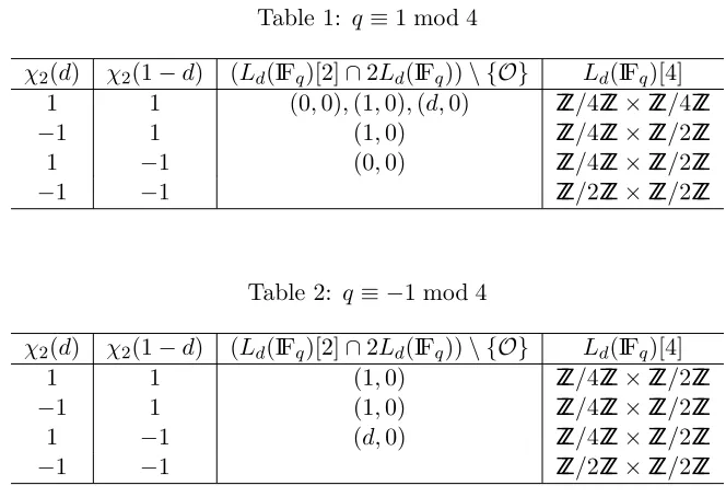
Applying Lemma 6.3 to the 2-torsion points (0,0),(1,0) and (d,0) of Ld(IFq),
Table 1: q ≡1 mod 4
χ2(d) χ2(1−d) (Ld(IFq)[2]∩2Ld(IFq))\ {O} Ld(IFq)[4]
1 1 (0,0),(1,0),(d,0) ZZ/4ZZ×ZZ/4ZZ
−1 1 (1,0) ZZ/4ZZ×ZZ/2ZZ
1 −1 (0,0) ZZ/4ZZ×ZZ/2ZZ
−1 −1 ZZ/2ZZ×ZZ/2ZZ
Table 2: q≡ −1 mod 4
χ2(d) χ2(1−d) (Ld(IFq)[2]∩2Ld(IFq))\ {O} Ld(IFq)[4]
1 1 (1,0) ZZ/4ZZ×ZZ/2ZZ
−1 1 (1,0) ZZ/4ZZ×ZZ/2ZZ
1 −1 (d,0) ZZ/4ZZ×ZZ/2ZZ
−1 −1 ZZ/2ZZ×ZZ/2ZZ
Lemma 6.4. Forq ≡ ±1 mod 4, the possible 4-torsion groups Ld(IFq)[4], are those
detailed in Tables 1 and 2 respectively.
We also use the following easy result, the first part of which was also used by Katz [11, Lemma 2.3].
Lemma 6.5. For d∈IFq\ {0,1} we have:
(i) A(d,IFq) =χ2(−1)·A(1−d,IFq),
(ii) A(d,IFq) =χ2(d)·A(1/d,IFq).
Proof. These are immediate consequences of isomorphisms (12) and (13). ut
We are now ready to prove our observations.
Theorem 6.6. Forq ≡1 (mod 4), let A be such that q+ 1−A≡0 (mod 8) (and so q+ 1 +A≡4 (mod 8)). Then Nn2(A) =Nn2(−A) =N(−A).
Proof. From Table 1 we see that for any square d, Ld(IFq) contains a subgroup of
order either 8 or 16. Asq+ 1 +A≡4 (mod 8), by Lagrange’s theorem we must have
N2(−A) = 0 . Hence alldcounted by N(−A) are necessarily non-square, and since
by Lemma 5.1 every unobstructed A occurs, we have Nn2(−A) = N(−A). Since
IFq\ {0,1,−1} partitions into a disjoint union of pairs {d,1/d}, by Lemma 6.5(ii)
for non-squaredwe have a bijection between the elements counted byNn2(−A) and
Theorem 6.7. Forq ≡ −1 (mod 4), we have
Nn2(A) = (
N(A) if q+ 1−A≡4 (mod 8)
N(A)/3 if q+ 1−A≡0 (mod 8).
Proof. We show that the result is true in each isomorphism class. First, assume
jL(d) 6= 0,1728, so that each isomorphism class contains the six distinct elements
in (14). From Table 2 we have that for any square d, Ld(IFq) contains a subgroup
of order 8. Hence if #Ld(IFq) = q+ 1−A ≡ 4 (mod 8), by Lagrange’s theorem
we must have N2(A) = 0. Hence all dcounted by N(A) are non-square, and since
every unobstructed A occurs, we have Nn2(A) =N(A). This proves the first part
of the theorem. For the second part, we shall show that for each A for which
q+ 1−A ≡0 (mod 8), square doccur twice as frequently as non-square din the counts for both N(A) and N(−A). Abusing notation slightly, when A(d,IFq) =A
we writed∈N(A), and simlarly for N(−A).
Let #Ld(IFq) = q+ 1−A≡0 (mod 8). Then by Sylow’s 1st theorem, Ld(IFq)
contains a subgroup of order 8, and hence Ld(IFq)[8] contains at least 8 points. By
Table 2, we can not have χ2(d) = χ2(1−d) = −1, since Ld(IFq)[4] ∼= ZZ2 ×ZZ2 = Ld(IFq)[2] and hence |Ld(IFq)[2i]| = 4 for i≥ 2. Hence we have three possibilities
for (χ2(d), χ2(1−d)).
Let χ2(d) = 1 with d∈ N(A). Then by Lemma 6.5(ii), 1/d ∈ N(A) also. By
Lemma 6.5(i), 1−d,1−1/d∈N(−A). Ifχ2(1−d) =−1 then by Lemma 6.5(ii) we
have 1/(1−d)∈N(A), andd/(d−1)∈N(−A). Hence {d,1/d,1/(1−d)} ∈N(A) and{1−d,1−1/d, d/(d−1)} ∈N(−A), and there are two squares and a non-square in each set, as asserted. If χ2(1−d) = 1 then by Lemma 6.5(ii) we have instead
1/(1−d)∈N(−A), and d/(d−1)∈N(A). Hence{d,1/d, d/(d−1)} ∈N(A) and
{1−d,1−1/d,1/(1−d)} ∈N(−A), and again there are two squares and a non-square in each set. Finally, ifχ2(d) =−1 andχ2(1−d) = 1, by Lemma 6.5 again we see that
ifd∈N(A) then{d,1−1/d, d/(d−1)} ∈N(A) and{1/d,1−d,1/(1−d)} ∈N(−A). In all cases N2(A) = 2Nn2(A) and N2(−A) = 2Nn2(−A), and the second part of
the result follows for these isomorphism classes.
If jL(d) = 1728, i.e., if d= 2,1/2,−1, it is easy to see that Lemma 6.5 implies
that the trace of Frobenius is zero in all cases. Nowχ2(2) =−1 ifq≡3 (mod 8) and
is 1 ifq ≡7 (mod 8). In the first case,q+ 1−0≡4 (mod 8) and this isomorphism class contributes three elements to Nn2(0) and hence N(0). In the second case q+ 1−0≡0 (mod 8) and this class contributes two squares and one non-square to
N(0).
If jL(d) = 0 then d2 −d+ 1 = 0, i.e., d and 1/d are primitive 6-th roots of
unity over IFq, which are in IFq iff q ≡1 (mod 6). Sinceq ≡ −1 (mod 4) we must
have q ≡7 (mod 12). In particular, IFq does not contain any 12-th roots of unity
and hence χ2(d) = −1. Since 1−d = 1/d, we have χ2(1−d) = χ2(1/d) = −1,
and so by Table 2, Ld(IFq)[4] ∼= ZZ2 ×ZZ2 and hence #Ld(IFq) = q + 1−A ≡ 4
this isomorphism class contributes one element toNn2(A) and henceN(A), and one
element toNn2(−A) and hence N(−A), whenever this isomorphism class is defined
over IFq. ut
Since by Lemma 5.1 we have N(A) >0 for every unobstructed integer A for a given q, we thus have the following.
Corollary 6.8. Let A be an unobstructed integer for q. Then there exists at least one quadratic non-residued∈IFq\ {0,1}such that #Ed(Fq) =q+ 1−A, and hence
there is a complete Edwards curve in every isogeny class.
Theorems 6.6 and 6.7 allow one can computeNn2(A) givenN(A), which can be
computed using Katz’s Deuring-style class number formula [11]. In fact for q ≡ 1 (mod 4), the formula forN(−A) is far simpler than that forN(A), while forq ≡ −1 (mod 4), N(A) and Nn2(A) are either equal or differ by a factor of 3.
To conclude this section, we note that Morain has independently proven the following [13, Theorem 17].
Theorem 6.9. LetE(IFp) :y2=x3+a2x2+a4x+a6 have threeIFp-rational2-torsion
points. Then there exists a curve E0(IFp) isogenous to E(IFp) that is birationally
equivalent to a complete Edwards curve.
Therefore, if such a curveE(IFq) exists in every isogeny class whose group order
is necessarily divisible by 4 =|E(IFq)[2]|, then Theorem 6.9 implies Corollary 6.8;
Theorem 2.2 provides the missing condition. Furthermore, Morain’s proof is con-structive, in that from such a curve E one can explicitly compute a set of isomor-phism classes of complete Edwards curves, based on the structure of the volcano of 2-isogenies of E.
7
Isogeny classes of
original
Edwards curves
As stated in §4.2, curves in Edwards’ original normal form (1) are isomorphic to the Bernstein-Lange form (2) via (x, y) 7→ (ax, ay), with d = a4. Two natural questions to consider are whether or not there exists an original Edwards curve in every isogeny class, and more specifically how are the original Edwards curves distributed amongst the isogeny classes? In this section we present answers to both these questions.
We begin with some definitions. For any unobstructed A for q, let N4(A) and N2n4(A) be the number of d∈ N(A) that are fourth powers, and squares but not
fourth powers, respectively. For any such A we thus have
N(A) =Nn2(A) +N2n4(A) +N4(A). (20)
Furthermore letχ4(·) denote a primitive biquadratic character of IFq, so thatχ4(d) =
7.1 Determining Ld(IFq)[8]
In the ensuing treatment, we will need to know the possible 8-torsion subgroups of
Ld(IFq). The structure of the 4-torsion was determined by analysing the halvability
of the 2-torsion points, using Lemma 6.3. Similarly, one can apply Lemma 6.3 to the elements of Ld(IFq)[4]\Ld(IFq)[2] to determine the structure of the 8-torsion.
Over the algebraic closure of IFq there are twelve points of order four; two for
each of the three 2-torsion points (0,0),(1,0) and (d,0):
P(0,0),± = (± √
d,√−1√d(1∓√d)), P(1,0),± = (1±
√
1−d,√1−d(1±√1−d)), P(d,0),± = (d±
p
d(d−1),pd(d−1)(√d±√d−1)),
along with their negatives (note that one can also prove Lemma 6.4 using these expressions). Applying Lemma 6.3 to these points gives:
Lemma 7.1. The following conditions are both necessary and sufficient for the points P(0,0),±, P(1,0),± and P(d,0),± respectively, to be halvable:
(i) P(0,0),±∈2Ld(IFq)⇐⇒ ±
√
d,±√d−1,±√d−d∈(IF×q)2, (ii) P(1,0),±∈2Ld(IFq)⇐⇒1±
√
1−d,±√1−d,1±√1−d−d∈(IF×q)2,
(iii) P(d,0),±∈2Ld(IFq)⇐⇒d± p
d(d−1), d±pd(d−1)−1,±pd(d−1)∈(IF×q)2.
7.2 The case q≡ −1 (mod 4)
This is the simplest case, giving rise to the following theorem:
Theorem 7.2. If q≡ −1 (mod 4), then the following holds:
(i) Let a4∈IFq\ {0,1}. Then #La4(IFq) =p+ 1−A≡0 (mod 8).
(ii) Conversely, if q+ 1−A≡0 (mod 8) then there exists a4 ∈ IFq\ {0,1} such
that#La4(IFq) =q+ 1−A.
(iii) If q+ 1−A≡0 (mod 8) then N4(A) =N2(A) = 2N(A)/3.
Proof. Since a4 is a square, by Table 2 we have La4(IFq)[4]∼=ZZ4×ZZ2, and hence
by Lagrange’s theorem we have 8 | #La4(IFq). This proves (i). Now let A be
any unobstructed integer satisfying q+ 1−A ≡ 0 (mod 8), and consider the set of all curves Ld(IFq) counted by N(A). By Lemma 5.1 this set is non-empty. By
Theorem 6.7 we have N2(A) = 2N(A)/3. Furthermore, since q ≡ −1 mod 4, the
7.3 The case q≡1 (mod 4)
We have the following theorem, which is proven in the remainder of this section:
Theorem 7.3. If q≡1 (mod 4), then the following holds:
(i) Let a4∈IFq\ {0,1}. Then #La4(IFq) =q+ 1−A≡0 (mod 16).
(ii) Conversely, if q+ 1−A≡0 (mod 16) then there exists a4 ∈IFq\ {0,1} such
that#La4(IFq) =q+ 1−A.
(iii) If q+ 1−A≡0 (mod 16) then N4(A) =N(A)−2N(−A).
Note that the implication in (iii) is equivalent toN4(A)/N(A) = 1−2/r, where r is Katz’s ratio N(A)/N(−A). Using Theorem 6.6 and (20), this is equivalent to
N4(A) =Nn2(A) +N2n4(A) +N4(A)−2Nn2(A), or
N2n4(A) =Nn2(A). (21)
Equation (21) in fact holds for all A such that q+ 1−A≡ 0 (mod 8), and seems to be non-trivial. We will prove it by constructing a bijection between the sets of curve parameters of each type. Once this equality is proven, part (ii) follows easily. The idea behind the proof of Equation (21) is a natural extension of the bijection-based proofs of§6 , which used the isomorphisms given in Lemma 6.5. Rather than use isomorphisms defined over IFq, which are isogenies of degree one, we use isogenies
of degree two. In particular we consider the isomorphism classes of curves arising from two 2-isogenies ofLd: the first being “divide by theZZ/2ZZ generated by (0,0)”
when d∈N2n4(A), and the second being “divide by theZZ/2ZZgenerated by (1,0)”
when d∈ Nn2(A), which are dual to one another. We begin with a short proof of
part (i).
Proof of (i): Let d = a4. Since χ2(d) = 1, by Table 1, if χ2(1−d) = 1 then Ld(IFq)[4] ≡ ZZ4 ×ZZ4 and hence 16 | #Ld(IFq). If χ2(1−d) = −1 then by Table
1 neither of (1,0) or (d,0) are halvable, and we claim that precisely one of P(0,0),±
is halvable. As χ2(−1) = 1, by Lemma 7.1, P(0,0),+ is halvable if and only if
√
d,√d−1 are both square, while P(0,0),− is halvable if and only if − √
d,−√d−1 are both square. Since χ4(d) = 1, both ±
√
d are square. Furthermore, as 1−d= (1 +√d)(1−√d) = (−√d−1)(√d−1), precisely one of these factors is square as
χ2(1−d) = −1 by assumption. This gives rise to a point of order 8. Therefore
ILd(IFq)[8]∼=ZZ8×ZZ2 and hence 16|#Ld(IFq) in this case too. This completes the
proof of (i).
We now exhibit a bijection to prove (21), assumingq+ 1−A≡0 (mod 8).
Proof. Note that if d∈N2n4(A) then by Table 1 we necessarily haveq+ 1−A≡0
(mod 8). Letξd:Ld→Ld/h(0,0)i and letEd=ξd(Ld). Using V´elu’s formula [17], Edhas equationy2=x3−(d+1)x2−4dx+4d(d+1) = (x−(d+1))(x−2√d)(x+2√d), and
ξd(x, y) = (x+d/x, y(1−d/x2)).
In particular, (1,0),(d,0)∈Ld are both mapped to (d+ 1,0)∈Ed, and hence Ldis
isomorphic to Ed/h(d+ 1,0)i.
Labelling the abscissae of the order 2 points of Ed bye1 =d+ 1, e2= 2
√
dand
e3=−2
√
d, one sees ([20]) thatEd has six isomorphic Legendre curves, each given
by a permutation of (e1, e2, e3) with paramaterλ= (e3−e1)/(e2−e1), and
(x, y)7→
x−e1 e2−e1
, y
(e2−e1)3/2
.
Each of these isomorphisms is defined over IFqif and only ifλ∈IFqandχ2(e2−e1) =
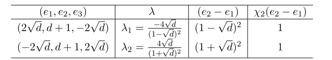
1 [20]. Ford∈N2n4(A), the twoEd-isomorphic Legendre curves used in the bijection
are given in Table 3.
Table 3: Ld/h(0,0)i-isomorphic Legendre curves in Nn2(A) for d∈N2n4(A)
(e1, e2, e3) λ (e2−e1) χ2(e2−e1)
(2√d, d+ 1,−2√d) λ1= −4
√
d
(1−√d)2 (1−
√
d)2 1 (−2√d, d+ 1,2√d) λ2= 4
√
d
(1+√d)2 (1 +
√
d)2 1
Observe that λ1(d), λ2(d)∈Nn2(A) sinceχ4(d)6= 1. Note also that λ1 = 1−δ,
with δ as given in §4.2, and hence this isomorphism class is precisely that of Ed;
indeed we have jL(δ) =jE(d). ThusEd∼=Ed, explaining our choice of notation.
Abusing notation slightly, we refer to the isomorphisms Ed→Lλ1(d) and Ed→
Lλ2(d) by λ1(d) and λ2(d) respectively. Note that bothλ1(d) and λ2(d) map (d+
1,0)∈Edto (1,0)∈Lλ1(d), Lλ2(d). Furthermore, ifdis replaced with 1/din Table
3, then each λi(d) remains invariant. HenceL1/d maps to λ1(d), λ2(d) as well, via ξ1/d(L1/d) =E1/d, and the point (1/d+ 1,0)∈E1/d maps to (1,0)∈Lλ1(d), Lλ2(d).
As 1/d∈N2n4(A), this means we have a map from the pair{d,1/d} ⊂N2n4(A) to
the pair{λ1(d), λ2(d)} ⊂Nn2(A). Note that d,1/d are distinct, unlessd=−1 and q ≡5 (mod 8), in which case we have λ1(−1) =λ2(−1) = 2 with χ2(2) = −1 and
hence 2∈Nn2(A). So in this exceptional case, we have an injection.
In the general case we thus have two pairs of maps:
with Lλ1(d) =Lλ1(1/d) and Lλ2(d) =Lλ2(1/d). We claim the above four maps taken
together form an injective map from pairs {d,1/d} to pairs {λ1(d), λ2(d)}. Indeed
suppose that ford0∈N2n4(A) we have
λ1(d0) =λ1(d) orλ2(d), orλ2(d0) =λ1(d) orλ2(d).
Then √d0 =±√d or√d0 =±1/√d, i.e., d0 =dor d0 = 1/d, and hence the map is
injective on the stated pairs. ut
Now consider the reverse direction, which is almost immediate.
Lemma 7.5. Let A satisfy q+ 1−A≡0 (mod 8). Then there exists an injection from Nn2(A) to N2n4(A).
Proof. Let e ∈ Nn2(A). For q+ 1−A ≡ 0 (mod 8), by Table 1 we must have χ2(e) =−1 and χ2(1−e) = 1. The only isomorphism defined over IFq in this case
maps Le −→ Le/(e−1) (see (15)). Therefore if e ∈ Nn2(A), then e−e1 ∈ Nn2(A).
Indeedλ2(d) =λ1(d)/(λ1(d)−1) (andλ1(d) =λ2(d)/(λ2(d)−1)).
Since λ1(d) andλ2(d) map the ˆξd-generating element (d+ 1,0) ofEdto (1,0) in Lλ1 and Lλ2 (and similarly (1/d+ 1,0)∈E1/d to (1,0)), the dual ˆξd of ξd applied
to the isomorphism class representative Le is given by Le/h(1,0)i, and similarly
for Le/(e−1). Hence if e = λ1(d) or λ2(d), then ˆξd maps elements of Nn2(A) to
the original isomorphism class of Ld. We now analyse this map and identify which
curves in the resulting isomorphism class are relevant.
For the sake of generality letγe:Le −→Le/h(1,0)i and let Fe =γe(Le). Using
V´elu’s formula Fe has equation y2 =x3−(e+ 1)x2−(6e−5)x−4e2 + 7e−3 = (x−(e−1))(x−(1 + 2√1−e))(x−(1−2√1−e)), and
γe(x, y) :=
x+ 1−e
x−1, y
1− 1−e
(x−1)2
.
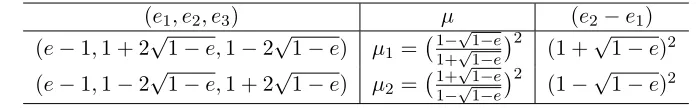
Note that γe(0,0) = γe(e,0) = (e−1,0). For e∈ Nn2(A), the two Fe-isomorphic
Legendre curves used in the bijection are given in Table 4.
Table 4: Two Le/h(1,0)i-isomorphic Legendre curves in N2n4(A) for e ∈ Nn2(A)
and q+ 1−A≡0 (mod 8)
(e1, e2, e3) µ (e2−e1)
(e−1,1 + 2√1−e,1−2√1−e) µ1= 1−
√
1−e 1+√1−e
2
(1 +√1−e)2 (e−1,1−2√1−e,1 + 2√1−e) µ2= 1+
√
1−e 1−√1−e
2
(1−√1−e)2
Observe thatχ2(e2−e1) = 1 in each case, and the same is true forµ1(e), µ2(e).
Furthermore,µ1(e), µ2(e) are both inN2n4(A) since (1±
√
square. Indeed, since 1−eis square, write 1−e=b2so thate= 1−b2= (1+b)(1−b). Therefore−1 =χ2(e) =χ2(1+b)χ2(1−b) =χ2(1+b)/χ2(1−b) =χ2((1+b)/(1−b)).
Again abusing notation slightly, we refer to the isomorphisms Fe →Lµ1(e) and Fe →Lµ2(e) by µ1(e) and µ2(e) respectively. Note that both µ1(e) andµ2(e) map
(e−1,0)∈Fe to (0,0)∈Lµ1(e), Lµ2(e). Furthermore, ifeis replaced with e/(e−1) in Table 4, then each µi(e) remains invariant. Hence Le/(e−1) maps to µ1(e), µ2(e)
as well, viaγe/(e−1)(Le/(e−1)) =Fe/(e−1), and the point (e/(e−1)−1,0)∈Fe/(e−1)
maps to (0,0)∈ Lµ1(e), Lµ2(e). As e/(e−1)∈ Nn2(A), this means we have a map
from the pair {e, e/(e−1)} ⊂ Nn2(A) to the pair {µ1(e), µ2(e)} ⊂ N2n4(A). Note
that e, e/(e−1) are distinct, unless e = 2 and q ≡ 5 (mod 8), in which case we have µ1(2) = µ2(2) = −1 with χ4(−1) 6= 1 and hence −1 ∈ N2n4(A). So in this
exceptional case, we have an injection (in fact the inverse of the previous injection). In the general case we thus have two pairs of maps:
µ1(e)◦γe:Le −→ Lµ1(e), µ2(e)◦γe:Le −→ Lµ2(e), µ1(e/(e−1))◦γe/(e−1):Le/(e−1) −→ Lµ1(e/(e−1)), µ2(e/(e−1))◦γe/(e−1):Le/(e−1) −→ Lµ2(e/(e−1)),
withLµ1(e) =Lµ1(e/(e−1)) and Lµ2(e)=Lµ2(e/(e−1)). We claim the above four maps
taken together form an injective map from pairs{e, e/(e−1)}to pairs{µ1(e), µ2(e)}.
Indeed suppose that fore0 ∈Nn2(A) we have
µ1(e0) =µ1(e) or µ2(e), orµ2(e0) =µ1(e) or µ2(e).
Thene0=eore0=e/(e−1), and hence the map is injective on the stated pairs. ut
We have thus proven:
Theorem 7.6. Let A satisfy q+ 1−A≡0 (mod 8). Then there exists a bijection between N2n4(A) and Nn2(A).
Furthermore, using the above definitions one can check that
µ1(λ1(d)) =µ1(λ2(d)) =d, and µ2(λ1(d)) =µ2(λ2(d)) = 1/d,
and similarly
λ1(µ1(e)) =λ1(µ2(e)) =e/(e−1), andλ2(µ1(e)) =λ2(µ2(e)) =e,
and that
(µ2(λ1(d))◦γλ1(d))◦(λ1(d)◦ξd) = [2] on Ld,
(µ2(λ2(d))◦γλ2(d))◦(λ2(d)◦ξd) = [2] on Ld,
(λ1(µ1(e))◦ξµ1(e))◦(µ1(e)◦γe) = [2] on Le,
Observe that if one substitutes d∈ N2n4(A) for ein the latter two maps, then
one obtains 2-isogenies from Ld to Lµ1(d),Lµ2(d), however µ1(d), µ2(d) 6∈ Nn2(A),
so the bijection can only be used in the manner proven. So while the bijection principally relies on a 2-isogeny and its dual, this alone is insufficient; one needs to also consider the isomorphism class representatives used, which is natural given that we are considering Legendre curve parameters drather than isomorphism classes of curves.
With regard to Theorem 7.3, note that Theorem 7.6 directly implies Theo-rem 7.3(iii). LetA be any unobstructed integer satisfyingq+ 1−A≡0 (mod 16), and consider the set of all curves Ld(IFq) counted by N(A). By Lemma 5.1 this set
is non-empty. Theorems 6.1 and 6.2 show that forq+ 1−A≡0 (mod 16) the ratio
N(A)/N(−A)>2 and thusN4(A) =N(A)−2N(−A)>0, which thus proves part
(ii) and completes the proof.
8
Curves defined using a ratio of two quadratics
Following on from §2 where we expressed the equation defining Ed in the form (7),
in this section we briefly discuss curves defined using a ratio of two quadratic poly-nomials or a ratio of a quadratic and a linear polynomial. We demonstrate that one can derive an addition formula for these types of curves and prove for them results similar to the results of the preceeding sections.
8.1 Ratio of two quadratics
Letf(x) =a1x2+b1x+c1, g(x) =a2x2+b2x+c2 ∈Fq[x] be as in Lemma 2.1,a1, a2
both non-zero, and define a curve by the equation
C/IFq :y2 =
a1x2+b1x+c1 a2x2+b2x+c2
. (22)
Notice that writing the curve equation as a ratio of two quadratics is just for the sake of the exposition and it is understood thatC/Fq is the projective curve defined
by the equation
(a2x2+b2xz+c2z2)y2=a1x2z2+b1xz3+c2z4.
Now suppose that
f(x) =a1(x−ω1)(x−ω2),
and
g(x) =a2(x−ω3)(x−ω4).
The conditions of Lemma 2.1 imply that ω1, ω2, ω3, ω4 are pairwise distinct. This
implies that there is a linear fractional transformation
φ:x7→ u1x+u2
u3x+u4
which mapsω1, ω2, ω3, ω4 toµ,−µ,1/µ,−1/µprovided that the cross-ratio condition
(ω1−ω3)(ω2−ω4)
(ω2−ω3)(ω1−ω4)
=
µ2−1
µ2+ 1 2
is satisfied (see [Chapter 4][14]). The map φinduces the map
ψ:x7→ −u4x+u2
u3x−u1
which in turn induces an isomorphism of the function field Fq(C) and the function
field of the curve Eµ,Fq(Eµ), where Eµ is defined by:
y2= x
2−µ2 x2− 1
µ2 .
Eµ is clearly isomorphic to the original Edwards curve (1). Thus Fq(C) is an
elliptic function field and hence the desingularization of C yields an elliptic curve. One can obtain results similar to the ones proven in [6] for the curveC. For example, one can obtain an addition formula for the points onC by using the Edwards curve addition formula and the mapφ, asφinduces a group homomorphism between the group of points onC and the group of points on Eµ.
8.2 Ratio of a quadratic and a linear polynomial
Now suppose that for the curve (22) we havea2 = 0, b2 6= 0, giving the corresponding
curve
C0/IFq:y2=
a1x2+b1x+c1 b2x+c2
. (23)
Then there is a linear fractional transformation
ϕ:x7→ u
0 1x+u
0 2 u03x+u04, u
0 i ∈IFq,
which maps C0 to a curve of the form 22 defined by a ratio of two quadratics, and which induces an isomorphism between the function fields ofC0 and a curve of the form 22. Thus our discussion in the previous section applies to curves defined using the ratio of a quadratic and a linear polynomial.
8.2.1 Huff curves
The Huff’s model of elliptic curves introduced by Huff [8] which has recently cap-tured the interest of the cryptographic community [9, 22] can be transformed to one of the form (23). In particular, the Huff’s curve, defined by the equation
is transformed to the curve
y2 = bt
2+at at+b ,
by setting xy =t. Thus one can generate the Huff’s curve addition law using the process outlined in the previous section. Furthermore, whenever a curve family is IFq-isomorphic to an Edwards or Legendre curve, one can deduce some properties
of the isogeny classes. For example, we have [22]
Ha,b∼=E a−b a+b
2 over IFq,
and so applying Theorems 6.6 and 6.7 we conclude that for any unobstructedA, if
q+ 1−A≡0 (mod 8) then there exists a Huff’s curve over IFq with that cardinality.
One can also apply the results of this paper directly to the Jacobi intersection family [5]
x2+y2 = 1 anddx2+z2= 1,
since this family hasj-invariantjL(d).
Remark 8.1. A new single-parameter family of elliptic curves was introduced in [18] (amongst more than 50,000others) defined by the curve equation
Ax+x2−xy2+ 1 = 0,
which enjoys a uniform x-coordinate addition formula. The curve equation can be rewritten as
y2= x
2+Ax+ 1
x .
Hence one can obtain addition formula for this family of curves using the addition law of Edwards curves, although we do not claim that this method generates the most efficient group law.
9
Concluding remarks
We have identified the set of isogeny classes of Edwards curves over finite fields of odd characteristic, and have found the proportion of parameters din each isogeny class which give rise to complete Edwards curves. Furthermore, we have identified the set of isogeny classes of original Edwards curves, and proven similar proportion results for this sub-family of curves.
Although not included in the paper, by analysing the 4- and 8-torsion of Legendre curves, and using variants of the established bijections, we were able to prove parts of Katz’s ratio theorems. We believe an interesting and challenging problem is whether or not the methods of this paper can be developed to provide an alternative proof for all parts of Katz’s ratio theorems; and conversely, can Katz’s methods be used to find relationships between N2k(A) and N(A) similar to those proven in
Acknowledgements
The authors would like to thank Steven Galbraith for offering some useful initial pointers, and for answering all our questions.
References
[1] Roland Auer and Jaap Top. Legendre elliptic curves over finite fields.J. Number Theory, 95(2):303–312, 2002.
[2] Daniel J. Bernstein, Peter Birkner, Marc Joye, Tanja Lange, and Christiane Peters. Twisted Edwards curves. InProgress in cryptology—AFRICACRYPT 2008, volume 5023 ofLecture Notes in Comput. Sci., pages 389–405. Springer, Berlin, 2008.
[3] Daniel J. Bernstein and Tanja Lange. Faster addition and doubling on elliptic curves. InAdvances in cryptology—ASIACRYPT 2007, volume 4833 of Lecture Notes in Comput. Sci., pages 29–50. Springer, Berlin, 2007.
[4] Ian F. Blake, Gadiel Seroussi, and Nigel P. Smart, editors. Advances in elliptic curve cryptography, volume 317 of London Mathematical Society Lecture Note Series. Cambridge University Press, Cambridge, 2005.
[5] D V Chudnovsky and G V Chudnovsky. Sequences of numbers generated by addition in formal groups and new primality and factorization tests.Adv. Appl. Math., 7:385–434, December 1986.
[6] Harold M. Edwards. A normal form for elliptic curves. Bull. Amer. Math. Soc. (N.S.), 44(3):393–422 (electronic), 2007.
[7] Reza Rezaeian Farashahi and Igor Shparlinski. On the number of distinct elliptic curves in some families. Des. Codes Cryptography, 54(1):83–99, 2010.
[8] Gerald B. Huff. Diophantine problems in geometry and elliptic ternary forms.
Duke Math. J., 15:443–453, 1948.
[9] Marc Joye, Mehdi Tibouchi, and Damien Vergnaud. Huff’s model for elliptic curves. Cryptology ePrint Archive, Report 2010/383, 2010. http://eprint. iacr.org/.
[10] Nicholas M. Katz. Lang-Trotter revisited. Bull. Amer. Math. Soc. (N.S.), 46(3):413–457, 2009.
[11] Nicholas M. Katz. 2, 3, 5, Legendre: ±trace ratios in families of elliptic curves.
[12] Dustin Moody and Daniel Shumow. Isogenies on edwards curves. preprint, 2010.
[13] Fran¸cois Morain. Edwards curves and CM curves. ArXiv e-prints, April 2009.
[14] Tristan Needham. Visual complex analysis. The Clarendon Press Oxford Uni-versity Press, New York, 1997.
[15] Joseph H. Silverman.The arithmetic of elliptic curves, volume 106 ofGraduate Texts in Mathematics. Springer-Verlag, New York, 1992. Corrected reprint of the 1986 original.
[16] John Tate. Endomorphisms of abelian varieties over finite fields.Invent. Math., 2:134–144, 1966.
[17] Jacques V´elu. Isog´enies entre courbes elliptiques. C. R. Acad. Sci. Paris S´er. A-B, 273:A238–A241, 1971.
[18] Fredrick Vercauteren and Wouter Castryck. Toric forms of elliptic curves and their arithmetic. Journal of Symbolic Computation, to appear.
[19] Z. X. Wang and D. R. Guo. Special functions. World Scientific Publishing Co. Inc., Teaneck, NJ, 1989. Translated from the Chinese by Guo and X. J. Xia.
[20] Lawrence C. Washington. Elliptic curves. Discrete Mathematics and its Appli-cations (Boca Raton). Chapman & Hall/CRC, Boca Raton, FL, 2003. Number theory and cryptography.
[21] Kenneth S. Williams. Finite transformation formulae involving the Legendre symbol. Pacific J. Math., 34:559–568, 1970.