An extended abstract of this paper appears in the Proceedings of Eurocrypt 2012, LNCS 7237, Springer. This is the full version.
Identity-Based (Lossy) Trapdoor Functions
and Applications
Mihir Bellare1 Eike Kiltz2 Chris Peikert3 Brent Waters4
May 2012
Abstract
We provide the first constructions of identity-based (injective) trapdoor functions. Furthermore, they are lossy. Constructions are given both with pairings (DLIN) and lattices (LWE). Our lossy identity-based trapdoor functions provide an automatic way to realize, in the identity-based setting, many functionalities previously known only in the public-key setting. In particular we obtain the first deterministic and efficiently searchable IBE schemes and the first hedged IBE schemes, which achieve best possible security in the face of bad randomness. Underlying our constructs is a new definition, namelypartial lossiness, that may be of broader interest.
1
Department of Computer Science & Engineering, University of California San Diego, 9500 Gilman Drive, La Jolla, CA 92093, USA. Email: mihir@cs.ucsd.edu. URL:http://cseweb.ucsd.edu/~mihir/. Supported in part by NSF grants CNS-0627779 and CCF-0915675.
2
Horst G¨ortz Institut f¨ur IT-Sicherheit, Ruhr-Universit¨at Bochum, D-44780 Bochum. Email: eike.kiltz@rub.de. URL:http://www.cits.rub.de/personen/kiltz.html.
3
School of Computer Science, College of Computing, Georgia Institute of Technology, 266 Ferst Drive, Atlanta, GA 30332-0765. Email: cpeikert@cc.gatech.edu. URL:http://www.cc.gatech.edu/~cpeikert/.
4
1
Introduction
A trapdoor function F specifies, for each public keypk, an injective,deterministic mapFpk that can be
inverted given an associated secret key (trapdoor). The most basic measure of security is one-wayness. The canonical example is RSA [55].
Suppose there is an algorithm that generates a “fake” public key pk∗ such that Fpk∗ is no longer
injective but has image much smaller than its domain and, moreover, given a public key, you can’t tell whether it is real or fake. Peikert and Waters [52] call such a TDF lossy. Intuitively, Fpk is close to a
functionFpk∗ that provides information-theoretic security. Lossiness implies one-wayness [52].
Lossy TDFs have quickly proven to be a powerful tool. Applications include IND-CCA [52], de-terministic [16], hedged [8] and selective-opening secure public-key encryption [10]. Lossy TDFs can be constructed from DDH [52], QR [35], DLIN [35], DBDH [24], LWE [52] and HPS (hash proof systems) [40]. RSA was shown in [44] to be lossy under the Φ-hiding assumption of [26], leading to the first proof of security of RSA-OAEP [13] without random oracles.
Lossy TDFs and their benefits belong, so far, to the realm of public-key cryptography. The purpose of this paper is to bring them to identity-based cryptography, defining and constructing identity-based TDFs (IB-TDFs), both one-way and lossy. We see this as having two motivations, one more theoretical, the other more applied, yet admittedly both foundational, as we discuss before moving further.
Theoretical angle. Trapdoor functions are the primitive that began public key cryptography [31, 55]. Public-key encryption was built from TDFs. (Via hardcore bits.) Lossy TDFs enabled the first DDH and lattice (LWE) based TDFs [52].
It is striking that identity-based cryptography developed entirely differently. The first realizations of IBE [21, 30, 58] directly used randomization and were neither underlain by, nor gave rise to, any IB-TDFs. We ask whether this asymmetry between the public-key and identity-based worlds (TDFs in one but not the other) is inherent. This seems to us a basic question about the nature of identity-based cryptography that is worth asking and answering.
Application angle. Is there anything here but idle curiosity? IBE has already been achieved without IB-TDFs, so why go backwards to define and construct the latter? The answer is that losssy IB-TDFs enable new applications that we do not know how to get in other ways.
Stepping back, identity-based cryptography [59] offers several advantages over its public-key coun-terpart. Key management is simplified because an entity’s identity functions as their public key. Key revocation issues that plague PKI can be handled in alternative ways, for example by usingidentity+date as the key under which to encrypt to identity [21]. There is thus good motivation to go beyond ba-sics like IBE [21, 30, 58, 17, 18, 62, 36] and identity-based signatures [11, 32] to provide identity-based counterparts of other public-key primitives.
Furthermore we would like to do this in a systematic rather than ad hoc way, leading us to seek tools that enable the transfer of multiple functionalities in relatively blackbox ways. The applications of lossiness in the public-key realm suggest that lossy IBTDFs will be such a tool also in the identity-based realm. As evidence we apply them to achieve based deterministic encryption and identity-based hedged encryption. The first, the counterpart of deterministic public-key encryption [7, 16], allows efficiently searchable identity-based encryption of database entries while maintaining the maximal possible privacy, bringing the key-management benefits of the identity-based setting to this application. The second, counterpart of hedged symmetric and public-key encryption [56, 8], makes IBE as resistant as possible in the face of low-quality randomness, which is important given the widespread deployment of IBE and the real danger of bad-randomness based attacks evidenced by the ones on the Sony Playstation and Debian Linux. We hope that our framework will facilitate further such transfers.
Contributions in brief. We define IB-TDFs and two associated security notions, one-wayness and lossiness, showing that the second implies the first.
The first wave of IBE schemes was from pairings [21, 58, 17, 18, 62, 61] but another is now emerging from lattices [36, 29, 2, 3]. We aim accordingly to reach our ends with either route and do so successfully. We provide lossy IB-TDFs from a standard pairings assumption, namely the Decision Linear (DLIN) assumption of [19]. We also provide IB-TDFs based on Learning with Errors (LWE) [53], whose hardness follows from the worst-case hardness of certain lattice-related problems [53, 50]. (The same assumption underlies lattice-based IBE [36, 29, 2, 3] and public-key lossy TDFs [52].) None of these results relies on random oracles.
Existing work brought us closer to the door with lattices, where one-way IB-TDFs can be built by combining ideas from [36, 29, 2]. Based on techniques from [50, 45] we show how to make them lossy. With pairings, however it was unclear how to even get a one-way IB-TDF, let alone one that is lossy. We adapt the matrix-based framework of [52] so that by populating matrix entries with ciphertexts of a very special kind of anonymous IBE scheme it becomes possible to implicitly specify per-identity matrices defining the function. No existing anonymous IBE has the properties we need but we build one that does based on methods of [23]. Our results with pairings are stronger because the lossy branches are universal hash functions which is important for applications.
Public-key lossy TDFs exist aplenty and IBE schemes do as well. It is natural to think one could easily combine them to get IB-TDFs. We have found no simple way to do this. Ultimately we do draw from both sources for techniques but our approaches are intrusive. Let us now look at our contributions in more detail.
New primitives and definitions. Public parameterspars and an associated master secret key having been chosen, an IB-TDF F associates to any identity a map Fpars,id, again injective and deterministic,
inversion being possible given a secret key derivable fromid via the master secret key. One-wayness means
Fpars,id∗ is hard to invert on random inputs for an adversary-specified challenge identityid∗. Importantly,
as in IBE, this must hold even when the adversary may obtain, via a key-derivation oracle, a decryption key for any non-challenge identity of its choice [21]. This key-derivation capability contributes significantly to the difficulty of realizing the primitive. As with IBE, security may be selective (the adversary must specify id∗ before seeing pars) [28] or adaptive (no such restriction) [21].
The most direct analog of the definition of lossiness from the public-key setting would ask that there be a way to generate “fake” parameters pars∗, indistinguishable from the real ones, such thatFpars∗,id∗ is
lossy (has image smaller than domain). In the selective setting, the fake parameter generation algorithm Pg∗ can takeid∗ as input, making the goal achievable at least in principle, but in the adaptive setting it is impossible to achieve, since, with id∗ not known in advance, Pg∗ is forced to make Fpars∗,id lossy for
all id, something the adversary can immediately detect using its key-derivation oracle.
We ask whether there is an adaptation of the definition of lossiness that is achievable in the adaptive case while sufficing for applications. Our answer is a definition of δ-lossiness, a metric of partial lossiness parameterized by the probabilityδthatFpars∗,id∗is lossy. The definition is unusual, involving an adversary
advantage that is the difference, not of two probabilities as is common in cryptographic metrics, but of two differently weighted ones. We will achieve selective lossiness with degree δ = 1, but in the adaptive case the best possible is degree 1/poly with the polynomial depending on the number of key-derivation queries of the adversary, and this what we will achieve. We show that lossiness with degree δ implies one-wayness, in both the selective and adaptive settings, as long as δ is at least 1/poly.
ID-LS-A ID-OW-A
ID-LS-S ID-OW-S
PK-LS PK-OW
Th 3.2
Th 3.2
[52]
Primitive δ Achieved under
ID-LS-A 1/poly DLIN, LWE ID-LS-S 1 DLIN, LWE
Figure 1: Types of TDFs based on setting (PK=Public-key,ID=identity-based), security (OW=one-way,LS=loss) and whether the latter is selective (S) or adaptive (A). An arrowA →B in the diagram on the left means that TDF of type Bis implied by (can be constructed from) TDF of type A. Boxed TDFs are the ones we define and construct. The table on the right shows the δ for which we prove δ-lossiness and the assumptions used. In both theSandAsettings theδwe achieve is best possible and suffices for applications.
ID-LS-A.
Closer Look. One’s first attempt may be to build an IB-TDF from an IBE scheme. In the random oracle (RO) model, this can be done by a method of [9], namely specify the coins for the IBE scheme by hashing the message with the RO. It is entirely unclear how to turn this into a standard model construct and it is also unclear how to make it lossy.
To build ID-TDFs from lattices we consider starting from the public-key TDF of [52] (which is already lossy) and trying to make it identity-based, but it is unclear how to do this. However, Gentry, Peikert and Vaikuntanathan (GPV) [36] showed that the function gA:Bαn+m →Znq defined by gA(x,e) =AT ·x+e
is a TDF for appropriate choices of the domain and parameters, where matrix A∈Zn×m
q is a uniformly
random public key which is constructed together with a trapdoor as for example in [4, 5, 46]. We make this function identity-based using the trapdoor extension and delegation methods introduced by Cash, Hofheinz, Kiltz and Peikert [29], and improved in efficiency by Agrawal, Boneh and Boyen [2] and Micciancio and Peikert [46]. Finally, we obtain a lossy IB-TDF by showing that this construction is already lossy.
With pairings there is no immediate way to get an IB-TDF that is even one-way, let alone lossy. We aim for the latter, there being no obviously simpler way to get the former. In the selective case we need to ensure that the function is lossy on the challenge identity id∗ yet injective on others, this setup being indistinguishable from the one where the function is always injective. Whereas the matrix diagonals in the construction of [52] consisted of ElGamal ciphertexts, in ours they are ciphertexts for identity id∗ under an anonymous IBE scheme, the salient property being that the “anonymity” property should hide whether the underlying ciphertext is to id∗ or is a random group element. Existing anonymous IBE schemes, in particular that of Boyen and Waters (BW) [23], are not conducive and we create a new one. A side benefit is a new anonymous IBE scheme with ciphertexts and private keys having one less group element than BW but still proven secure under DLIN.
A method of Boneh and Boyen [17] can be applied to turn selective into adaptive security but the reduction incurs a factor that is equal to the size of the identity space and thus ultimately exponential in the security parameter, so that adaptive security according to the standard asymptotic convention would not have been achieved. To achieve it, we want to be able to “program” the public parameters so that they will be lossy on about a 1/Q fraction of “random-ish” identities, whereQ is the number of key-derivation queries made by the attacker. Ideally, with probability around 1/Q all of (a successful) attacker’s queries will land outside the lossy identity-space, but the challenge identity will land inside it so that we achieve δ-lossiness withδ around 1/Q.
partitioning of the identities into two classes was based solely on the reduction algorithm’s internal view of the public parameters; the parameters themselves were distributed independently of this partitioning and thus the adversary view was the same as in a normal setup. In contrast, the partitioning in our scheme will actually directly affect the parameters and how the system behaves. This is why we must rely on a computational assumption to show that the partitioning in undetectable. A key novel feature of our construction is the introduction of a system that will produce lossy public parameters for about a 1/Qfraction of the identities.
Applications. Deterministic PKE is a TDF providing the best possible privacy subject to being deter-ministic, a notion called PRIV that is much stronger than one-wayness [7]. An application is encryption of database records in a way that permits logarithmic-time search, improving upon the linear-time search of PEKS [20]. Boldyreva, Fehr and O’Neill [16] show that lossy TDFs whose lossy branch is a universal hash (called universal lossy TDFs) achieve (via the LHL [15, 39]) PRIV-security for message sequences which are blocksources, meaning each message has some min-entropy even given the previous ones, which remains the best result without ROs. Deterministic IBE and the resulting efficiently-searchable IBE are attractive due to the key-management benefits. We can achieve them because our DLIN-based lossy IB-TDFs are also universal lossy. (This is not true, so far, for our LWE based IB-TDFs.)
To provide IND-CPA security in practice, IBE relies crucially on the availability of fresh, high-quality randomness. This is fine in theory but in practice RNGs (random number generators) fail due to poor entropy gathering or bugs, leading to prominent security breaches [37, 38, 25, 49, 48, 1, 63, 33]. Expecting systems to do a better job is unrealistic. Hedged encryption [8] takes poor randomness as a fact of life and aims to deliver best possible security in the face of it, providing privacy as long as the message together with the “randomness” have some min-entropy. Hedged PKE was achieved in [8] by combining IND-CPA PKE with universal lossy TDFs. We can adapt this to IBE and combine existing (randomized) IBE schemes with our DLIN-based universal lossy IB-TDFs to achieved hedged IBE. This is attractive given the widespread use of IBE in practice and the real danger of randomness failures.
Both applications are for the case of selective security. We do not achieve them in the adaptive case. Related Work. A number of papers have studied security notions of trapdoor functions beyond traditional one-wayness. Besides lossiness [52] there is Rosen and Segev’s notion of correlated-product security [57], and Canetti and Dakdouk’s extractable trapdoor functions [27]. The notion of adaptive one-wayness for tag-based trapdoor functions from Kiltz, Mohassel and O’Neill [43] can be seen as the special case of our selective IB-TDF in which the adversary is denied key-derivation queries. Security in the face of these queries was one of the main difficulties we faced in realizing IB-TDFs.
Organization. We define IB-TDFs, one-wayness andδ-lossiness in Section 2. We also define extended IB-TDFs, an abstraction that will allow us to unify and shorten the analyses for the selective and adaptive security cases. In Section 3 we show that δ-lossiness implies one-wayness as long as δ is at least 1/poly. This allows us to focus on achieving δ-lossiness. In Section 4 we provide our pairing-based schemes and in Appendix 5 our lattice-based schemes. In Appendix B we sketch how to apply δ-lossy IB-TDFs to achieve deterministic and hedged IBE.
Subsequent work. Escala, Herranz, Libert and R´afols [34] provide an alternative definition of partial lossiness based on which they achieve deterministic, PRIV-secure IBE for blocksources, and hedged IBE, in the adaptive case, which answers an open question from our work. They also define and construct hierarchical identity-based (lossy) trapdoor functions.
2
Definitions
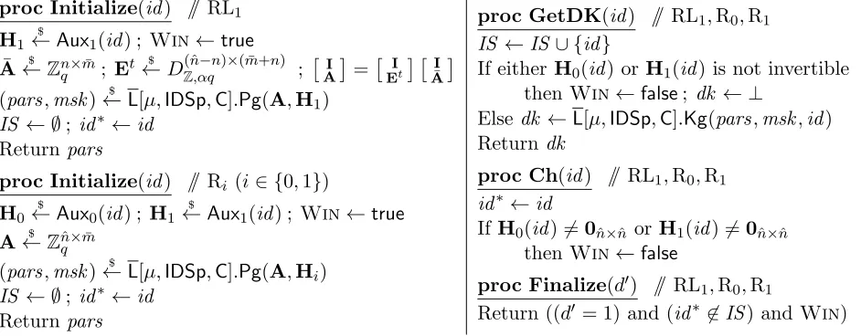
proc Initialize(id) // OWF,RealF (pars,msk)←$ F.Pg; IS ← ∅; id∗ ←id Return pars
proc GetDK(id) // OWF,RealF
IS ←IS ∪ {id}
dk ←F.Kg(pars,msk,id) Return dk
proc Ch(id) // OWF
id∗←id ; x←$ InSp
y ←F.Ev(pars,id∗, x) Return y
proc Finalize(x′) // OWF Return ((x′ =x) and (id∗6∈IS))
proc Initialize(id) // LossyF,LF,ℓ
(pars,msk)←$ LF.Pg(id) ; IS ← ∅; id∗← id Returnpars
proc GetDK(id) // LossyF,LF,ℓ
IS ←IS ∪ {id}
dk ←LF.Kg(pars,msk,id) Returndk
proc Ch(id) // RealF,LossyF,LF,ℓ
id∗←id
proc Finalize(d′) // RealF Return ((d′ = 1) and (id∗6∈IS)) proc Finalize(d′) // LossyF,LF,ℓ
Return ((d′ = 1) and (id∗6∈IS) and (λ(F.Ev(pars,id∗,·))≥ℓ))
Figure 2: Games defining one-wayness and δ-lossiness of IBTDFF with associated siblingLF.
empty string is denoted ε. IfS is a set then |S| denotes its size, Sa denotes the set of a-vectors over S,
Sa×b denotes the set ofabybmatrices with entries inS, and so on. The (i, j)-th entry of a 2 dimensional
matrix Mis denoted M[i, j] and the (i, j, k)-th entry of a 3 dimensional matrixM is denotedM[i, j, k]. If M is a n by µ matrix then M[j,·] denotes the vector (M[j,1], . . . ,M[j, µ]). If a = (a1, . . . , an)
then (a1, . . . , an) ← a means we parse a as shown. Unless otherwise indicated, an algorithm may be
randomized. By y ←$ A(x1, x2, . . .) we denote the operation of runningA on inputs x1, x2, . . . and fresh coins and letting y denote the output. We denote by [A(x1, x2, . . .)] the set of all possible outputs of A on inputsx1, x2, . . .. The (Kronecker) delta function ∆ is defined by ∆(a, b) = 1 ifa=band 0 otherwise. Ifa, bare equal-length vectors of reals thenha, bi=a[1]b[1] +· · ·+a[|a|]b[|b|] denotes their inner product. Games. A game —look at Figure 2 for an example— has anInitializeprocedure, procedures to respond to adversary oracle queries, and aFinalizeprocedure. To execute a game G is executed with an adversary
A means to run the adversary and answer its oracle queries by the corresponding procedures of G. The adversary must make exactly one query to Initialize, this being its first oracle query. (This means the adversary can give Initializean input, an extension of the usual convention [14].) It must make exactly one query to Finalize, this being its last oracle query. The reply to this query, denoted GA, is called the output of the game, and we let “GA” denote the event that this game output takes valuetrue. Boolean flags are assumed initialized to false.
IBTDFs. An identity-based trapdoor function (IBTDF) is a tuple F = (F.Pg,F.Kg,F.Ev,F.Ev−1) of algorithms with associated input spaceInSpand identity spaceIDSp. The parameter generation algorithm F.Pg takes no input and returns common parameters pars and a master secret key msk. On input pars,msk,id, the key generation algorithm F.Kgproduces a decryption key dk for identity id. For any pars and id ∈IDSp, the deterministic evaluation algorithmF.Ev defines a function F.Ev(pars,id,·) with domain InSp. We requirecorrect inversion: For any pars, any id ∈IDSp and any dk ∈[F.Kg(pars,id)], the deterministic inversion algorithm F.Ev−1 defines a function that is the inverse of F.Ev(pars,id,·), meaning F.Ev−1(pars,id,dk,F.Ev(pars,id, x)) =x for all x∈InSp.
these induced schemes need, however, satisfy the correct inversion requirement. If the one induced by aux does, we say thataux grants invertibility. Looking ahead we will build an E-IBTDF and then obtain our IBTDF as the one induced by a particular auxiliary input, the other induced schemes being the basis of the siblings and being used in the proof.
One-wayness. One-wayness of IBTDF F = (F.Pg,F.Kg,F.Ev,F.Ev−1) is defined via game OWF of Figure 2. The adversary is allowed only one query to its challenge oracle Ch. The advantage of such an adversary I isAdvowF (I) = Pr
OWIF
.
Selective versus adaptive ID.We are interested in both these variants for all the notions we consider. To avoid a proliferation of similar definitions, we capture the variants instead via different adversary classes relative to the same game. To exemplify, consider game OWF of Figure 2. Say that an adversary
A is selective-id if the identity id in its queries to Initialize and Ch is always the same, and say it is adaptive-id if this is not necessarily true. Selective-id security for one-wayness is thus captured by restricting attention to selective-id adversaries and full (adaptive-id) security by allowing adaptive-id adversaries. Now, adopt the same definitions of selective and adaptive adversaries relative to any game that provides procedures called Initialize and Ch, regardless of how these procedures operate. In this way, other notions we will introduce, including partial lossiness defined via games also in Figure 2, will automatically have selective-id and adaptive-id security versions.
Partial lossiness. We first provide the formal definitions and later explain them and their relation to standard definitions. If f is a function with domain a (non-empty) set Dom(f) then its image is Im(f) ={f(x) : x∈Dom(f)}. We define thelossiness λ(f) off via
λ(f) = lg|Dom(f)|
|Im(f)| or equivalently |Im(f)|=|Dom(f)| ·2−
λ(f).
We say that f is ℓ-lossy if λ(f) ≥ ℓ. Let IBTDF F = (F.Pg,F.Kg,F.Ev,F.Ev−1) be an IBTDF with associated input space InSpand identity spaceIDSp. Asibling forFis an E-IBTDFLF= (LF.Pg,LF.Kg,
F.Ev,F.Ev−1) whose evaluation and inversion algorithms, as the notation indicates, are those of F and whose auxiliary input space is IDSp. Algorithm LF.Pg will use this input in the selective-id case and ignore it in the adaptive-id case. Consider games RealF and LossyF,LF,ℓ of Figure 2. The first uses the real parameter and key-generation algorithms while the second uses the sibling ones. A los-adversary A
is allowed just one Ch query, and the games do no more than record the challenge identity id∗. The advantage of the adversary isnot, as usual, the difference in the probabilities that the games returntrue, but is instead parameterized by a probability δ∈[0,1]and defined via
AdvδF-los,LF,ℓ(A) =δ·Pr
RealAF
−Pr
LossyAF,LF,ℓ
. (1)
Discussion. The PW [52] notion of lossy TDFs in the public-key setting asks for an alternative “sibling” key-generation algorithm, producing a public key but no secret key, such that two conditions hold. The first, which is combinatorial, asks that the functions defined by sibling keys are lossy. The second, which is computational, asks that real and sibling keys are indistinguishable. The first change for the IB setting is that one needs an alternative parameter generation algorithm which produces not onlypars but a master secret keymsk, and an alternative key-generation algorithm that, based onmsk, can issue decryption keys to users. Now we would like to ask that the function F.Ev(pars,id∗,·) be lossy on the challenge identity id∗ whenpars is generated viaLF.Pg, but, in the adaptive-id case, we do not knowid∗ in advance. Thus the requirement is made via the games.
We would like to define the advantage normally, meaning withδ = 1, but the resulting notion is not achievable in the adaptive-id case. (This can be shown via attack.) With the relaxation, a low (close to zero) advantage means that the probability that the adversary finds a lossy identity id∗ and then outputs 1 is less than the probability that it merely outputs 1 by a factor not much less thanδ. Roughly, it means that a δ fraction of identities are lossy. The advantage represents the computational loss while
IBE. Recall that an IBE scheme IBE = (IBE.Pg,IBE.Kg,IBE.Enc,IBE.Dec) is a tuple of algorithms with associated message space InSp and identity space IDSp. The parameter generation algorithm IBE.Pg takes no input and returns common parameters pars and a master secret key msk. On in-put pars,msk,id, the key generation algorithm IBE.Kg produces a decryption key dk for identity id. On input pars, id ∈ IDSp and a message M ∈ InSp the encryption algorithm IBE.Enc returns a ci-phertext. The decryption algorithm IBE.Dec is deterministic. The scheme has decryption error ǫ if Pr[IBE.Dec(pars,id,dk,IBE.Enc(pars,id, M))6=M]≤ǫfor allpars, allid ∈IDSp, alldk ∈[F.Kg(pars,id)] and allM ∈InSp. We say thatIBEis deterministic ifIBE.Encis deterministic. A deterministic IBE scheme is identical to an IBTDF.
3
Implications of Partial Lossiness
Theorem 3.2 shows that partial lossiness implies one-wayness. We discuss other applications in Ap-pendix B. We first need a simple lemma.
Lemma 3.1 Let f be a function with non-empty domain Dom(f). Then for any adversary A
Pr[A(y) =x : x←$ Dom(f) ; y←f(x)] ≤ 2−λ(f).
Proof of Lemma 3.1: Fory∈Im(f) letf−1(y) be the set of all x∈Dom(f) such thatf(x) =y. The probability in question is
X
y∈Im(f)
Pr [A(y) =x | f(x) =y]·Pr [f(x) =y] ≤ X
y∈Im(f) 1
|f−1(y)| ·
|f−1(y)| |Dom(f)| =
|Im(f)| |Dom(f)| = 2
−λ(f)
where the probability is over x chosen at random from Dom(f) and the coins of A if any. (Since A is unbounded, it can be assumed wlog to be deterministic.)
Theorem 3.2 [ δ-lossiness implies one-wayness ] Let F = (F.Pg,F.Kg,F.Ev,F.Ev−1) be a IBTDF with associated input space InSp. LetLF= (LF.Pg,LF.Kg,F.Ev,F.Ev−1)be a lossy sibling for F. Letδ >0 and let ℓ≥0. Then for any ow-adversary I there is a los-adversary A such that
AdvowF (I)≤
AdvδF-,LFlos,ℓ(A) + 2−ℓ
δ . (2)
The running time of A is that if I plus the time for a computation of F.Ev. If I is a selective adversary then so is A.
In asymptotic terms, the theorem says that δ-lossiness implies one-wayness as long as δ−1 is bounded above by a polynomial in the security parameter and ℓis super-logarithmic. This means δ need only be non-negligible. The last sentence of the theorem, saying that if I is selective then so is A, is important because it says that the theorem covers both the selective and adaptive security cases, meaning selective
δ-lossiness implies selective one-wayness and adaptive δ-lossiness implies adaptive one-wayness.
Proof of Theorem 3.2: AdversaryA runs I. When I makes queryInitialize(id), adversary A does the same, obtaining pars and returning this to I. AdversaryA answers I’s queries to itsGetDK oracle via its own oracle of the same name. When I makes its (single)Ch query id∗, adversary A also makes query Ch(id∗). Additionally, it picks x at random from InSp and returns y = F.Ev(pars,id∗, x) to I. The latter eventually halts with output x′. Adversary A returns 1 if x′ =x and 0 otherwise. By design we clearly have Pr
RealAF
= AdvowF (I). But game LossyF,LF,ℓ returns true only if F.Ev(pars,id∗,·) is
ℓ-lossy, in which case the probability that x=x′ is small by Lemma 3.1. In detail, assuming wlog thatI
never queries id∗ to GetDK, we have Pr
LossyAF,LF,ℓ
= Pr
x=x′ | λ(F.Ev(pars,id∗,·))≥ℓ
·Pr [λ(F.Ev(pars,id∗,·))≥ℓ]
≤ Pr
x=x′ | λ(F.Ev(pars,id∗,·))≥ℓ
the last inequality by Lemma 3.1 applied to the function f = F.Ev(pars,id∗,·). From Equation (1) we have
AdvδF-los,LF,ℓ(A) = δ·Pr
RealAF
−Pr
LossyAF,LF,ℓ
≥ δ·AdvowF (I)−2−ℓ .
Equation (2) follows. In Section B we discuss the application to deterministic and hedged IBE.
4
IB-TDFs from pairings
In Section 3 we show that δ-lossiness implies one-wayness in both the selective and adaptive cases. We now show how to achieve δ-lossiness using pairings.
Setup. Throughout we fix a bilinear mape: G×G → GT where G,GT are groups of prime order p. By 1,1T we denote the identity elements ofG,GT, respectively. By G∗ =G− {1} we denote the set of
generators of G. The advantage of a dlin-adversary B is
Advdlin(B) = 2 Pr[DLINB]−1,
where game DLIN is as follows. The Initialize procedure picks g,gˆ at random from G∗, s at random from Z∗
p, ˆs at random from Zp and X at random from G. It picks a random bit b. If b = 1 it lets
T ← Xs+ˆs and otherwise picks T at random from G. It returns (g,ˆg, gs,ˆgsˆ, X, T) to the adversary B. The adversary outputs a bit b′ and Finalize, given b′ returns true if b = b′ and false otherwise. For integer µ≥1, vectors U∈Gµ+1 and y∈Zµp+1, and vector id ∈Zµp we let
id = (1,id[1], . . . ,id[µ])∈Zpµ+1 and H(U,id) =Qµ
k=0U[k]
id[k].
H is the BB hash function [17] when µ = 1, and the Waters’ one [23] when IDSp = {0,1}µ and an
id ∈IDSp is viewed as a µ-vector over Zp. We also let
f(y,id) =Pµ
k=0y[k]id[k] and f(y,id) =f(y,id) modp .
4.1 Overview
In the Peikert-Waters [52] design, the matrix entries are ciphertexts of an underlying homomorphic encryption scheme, and the function output is a vector of ciphertexts of the same scheme. We begin by presenting an IBE scheme, that we call the basic IBE scheme, such that the function outputs of our eventual IB-TDF will be a vector of ciphertexts of this IBE scheme. Towards building the IB-TDF, the first difficulty we run into in setting up the matrix is that ciphertexts depend on the identity and we cannot have a different matrix for every identity. Thus, our approach is more intrusive. We will have many matrices which contain certain “atoms” from which, given an identity, one can reconstruct ciphertexts of the IBE scheme. The result of this intrusive approach is that security of the IB-TDF relies on more than security of the base IBE scheme. Our ciphertext pseudorandomness lemma (Lemma 4.1) shows something stronger, namely that even the atoms from which the ciphertexts are created look random under DLIN. This will be used to establish Lemma 4.2, which moves from the real to the lossy setup. The heart of the argument is the proofs of the lemmas, which are in the appendices.
4.2 Our basic IBE scheme
We associate to any integer µ ≥ 1 and any identity space IDSp ⊆Zµp an IBE scheme IBE[µ,IDSp] that has message space {0,1} and algorithms as follows:
1. Parameters: AlgorithmIBE[µ,IDSp].Pgletsg←$ G∗;t←$ Zp∗; ˆg←gt. It then letsH,Hˆ ←$ G;U,Uˆ ←$ Gµ+1. It returnspars = (g,g, H,ˆ H,ˆ U,Uˆ) as the public parameters andmsk =tas the master secret key.
2. Key generation:Given parameters (g,g, H,ˆ H,ˆ U,Uˆ), master secrettand identityid ∈IDSp, algorithm IBE[µ,IDSp].Kgreturns decryption key (D1, D2, D3, D4) computed by lettingr,ˆr
$
←Zp and setting
D1← H(U,id)tr·Htrˆ; D2 ← H(Uˆ,id)r·Hˆrˆ; D3 ←g−tr; D4 ←g−tˆr.
3. Encryption:Given parameters (g,ˆg, H,H,ˆ U,Uˆ), identityid ∈IDSpand messageM ∈ {0,1}, algorithm IBE[µ,IDSp].Enc returns ciphertext (C1, C2, C3, C4) computed as follows. IfM = 0 then it letss,sˆ
$
←
Zp andC1 ←gs;C2 ←ˆgsˆ;C3← H(U,id)s·H(Uˆ,id)ˆs;C4 ←HsHˆsˆ. IfM = 1 it letsC1, C2, C3, C4←$ G.
4. Decryption: Given parameters (g,ˆg, H,H,ˆ U,Uˆ), identity id ∈IDSp, decryption key (D1, D2, D4, D4) for id and ciphertext (C1, C2, C3, C4), algorithm IBE[µ,IDSp].Dec returns 0 if e(C1, D1)e(C2, D2) e(C3, D3)e(C4, D4) =1T and 1 otherwise.
This scheme has non-zero decryption error (at most 2/p) yet our IBTDF will have zero inversion error. This scheme turns out to be IND-CPA+ANON-CPA although we will not need this in what follows. Instead we will have to consider a distinguishing game related to this IBE scheme and our IBTDF. In Appendix A we give a (more natural) variant of IBE[µ,IDSp] that is more efficient and encrypts strings rather than bits. The improved IBE scheme can still be proved IND-CPA+ANON-CPA but it cannot be used for our purpose of building IB-TDFs.
4.3 Our E-IBTDF and IB-TDF
Our E-IBTDF E[n, µ,IDSp] is associated to any integers n, µ≥1 and any identity space IDSp⊆Zµp. It has message space {0,1}n and auxiliary input spaceZµ+1
p , and the algorithms are as follows:
1. Parameters:Given auxiliary inputy, algorithmE[n, µ,IDSp].Pgletsg←$ G∗;t←$ Z∗p; ˆg←gt;U ←$ G∗. It then lets H,Hˆ ←$ Gn; V,Vˆ ←$ Gn×(µ+1) and s ←$ (Z∗
p)n; ˆs
$
← Zn
p. It returns pars = (g,g,ˆ G,
ˆ
G,J,W,H,Hˆ,V,Vˆ, U) as the public parameters and msk = t as the master secret key where for 1≤i, j≤nand 0≤k≤µ:
G[i]←gs[i]; Gˆ[i]←gˆˆs[i]; J[i, j]←H[j]s[i]Hˆ[j]ˆs[i]; W[i, j, k]←V[j, k]s[i]Vˆ[j, k]ˆs[i]Us[i]y[k]∆(i,j),
where we recall that ∆(i, j) = 1 ifi=j and 0 otherwise is the Kronecker Delta function.
2. Key generation: Given parameters (g,ˆg,G,Gˆ,J,W,H,Hˆ,V,Vˆ, U), master secret tand identity id ∈
IDSp, algorithm E[n, µ,IDSp].Kg returns decryption key (D1,D2,D3,D4) where r $
← (Z∗
p)n;ˆr
$
←Zn
p
and for 1≤i≤n
D1[i]← H(V[i,·],id)tr[i]·H[i]tˆr[i];D2[i]← H(Vˆ[i,·],id)r[i]·Hˆ[i]ˆr[i]; D3[i]←g−tr[i]; D4[i]←g−tˆr[i]. 3. Evaluate: Given parameters (g,ˆg,G,Gˆ,J,W,H,Hˆ,V,Vˆ, U), identity id ∈ IDSp and input x ∈
{0,1}n, algorithmE[n, µ,IDSp].Ev returns (C
1, C2,C3,C4) where for 1≤j≤n
C1 ←Qni=1G[i]x[i]; C2 ←Qni=1Gˆ[i]x[i];C3[j]←Qni=1Qµk=0W[i, j, k]x[i]id[k]; C4[j]←Qni=1J[i, j]x[i] 4. Invert: Given parameters (g,g,ˆ G,Gˆ,J,W,H,Hˆ,V,Vˆ, U), identity id ∈ IDSp, decryption key (D1,
{0,1}n where for 1≤j≤nit sets x[j] = 0 if e(C
1,D1[j])e(C2,D2[j])e(C3[j],D3[j])e(C4[j],D4[j]) = 1T and 1 otherwise.
Invertibility. We observe that if parameters (g,g,ˆ G,Gˆ,J,W,H,Hˆ,V,Vˆ, U) were generated with auxiliary inputy and (C1, C2,C3,C4) =E[n, µ,IDSp].Ev((g,g,ˆ G,Gˆ,J,W),id, x) then for 1≤j ≤n
C1 = Qni=1gs[i]x[i]=ghs,xi (3)
C2 = Qni=1gˆˆs[i]x[i]= ˆghˆs,xi (4)
C3[j] = Qni=1
Qµ
k=0V[j, k]s[i]x[i]id[k]Vˆ[j, k]ˆs[i]x[i]id[k]Us[i]x[i]y[k]id[k]∆(i,j) = Qn
i=1H(V[j,·],id)s[i]x[i]H(Vˆ[j,·],id)ˆs[i]x[i]Us[i]x[i]f(y,id)∆(i,j)
= H(V[j,·],id)hs,xiH(Vˆ[j,·],id)hˆs,xiUs[j]x[j]f(y,id) (5) C4[j] = Qni=1H[j]s[i]x[i]Hˆ[j]ˆs[i]x[i]=H[j]hs,xiHˆ[j]hˆs,xi. (6) Thus if x[j] = 0 then (C1, C2,C3[j],C4[j]) is an encryption, under our base IBE scheme, of the mes-sage 0, with coins hs, ximodp,hˆs, ximodp, parameters (g,g,ˆ H[j],Hˆ[j],V[j,·],Vˆ[j,·]) and identity id. The inversion algorithm will thus correctly recover x[j] = 0. On the other hand suppose x[j] = 1. Then e(C1,D1[j])e(C2,D2[j])e(C3[j],D3[j])e(C4[j],D4[j]) = e(Us[j]x[j]f(y,id),D3[j]). Now suppose
f(y,id) modp= 0. Then6 Us[j]x[j]f(y,id)6=1because we choses[j] to be non-zero modulopandD
3[j]6=1 because we chose r[j] to be non-zero modulo p. So the result of the pairing is never 1T, meaning the
inversion algorithm will again correctly recover x[j] = 1. We have established that auxiliary input y grants invertibility, meaning induced IBTDF E[n, µ,IDSp](y) satisfies the correct inversion condition, if
f(y,id) modp6= 0 for allid ∈IDSp.
Our IBTDF. We associate to any integers n, µ ≥ 1 and any identity space IDSp ⊆ Zµp the IBTDF scheme induced by our E-IBTDF E[n, µ,IDSp] via auxiliary input y= (1,0, . . . ,0) ∈Zµp+1, and denote this IBTDF scheme by F[n, µ,IDSp]. This IBTDF satisfies the correct inversion requirement because
f(y,id) = id[0] = 1 6≡0 (mod p) for all id. We will show that this IBTDF is selective-id secure when
µ = 1 and IDSp = Zp, and adaptive-id secure when IDSp = {0,1}µ. In the first case, it is fully lossy (i.e. 1-lossy) and in the second it is δ-lossy for appropriate δ. First we prove two technical lemmas that we will use in both cases.
4.4 Ciphertext pseudorandomness lemma
Consider games ReC,RaC of Figure 3 associated to some choice of IDSp⊆Zµp. The adversary provides the Initialize procedure with an auxiliary input y ∈ Zµp+1. Parameters are generated as per our base IBE scheme with the addition of U. The decryption key for id is computed as per our base IBE scheme except that the games refuse to provide it when f(y,id) = 0. The challenge oracle, however, does not return ciphertexts of our IBE scheme. In game ReC, it returns group elements that resemble diagonal entries of the matrices in the parameters of our E-IBTDF, and in game RaC it returns random group elements. Notice that the challenge oracle does not take an identity as input. (Indeed, it has no input.) As usual it must be invoked exactly once. The following lemma says the games are indistinguishable under DLIN. The proof is in Section 4.7.
Lemma 4.1 Let µ≥1be an integer andIDSp⊆Zµp. LetP be an adversary. Then there is an adversary
B such that
Pr
ReCP
−Pr
RaCP
≤ (µ+ 2)·Advdlin(B). (7)
proc Initialize(y) // ReC,RaC (pars,msk)←$ IBE[µ,IDSp].Pg (g,g, H,ˆ H,ˆ U,Uˆ)←pars
U ←$ G∗
Return (g,g, H,ˆ H,ˆ U,Uˆ, U) proc GetDK(id) // ReC,RaC Iff(y,id) = 0 thendk ← ⊥
Elsedk ←IBE[µ,IDSp].Kg(pars,msk,id) Returndk
proc Ch() // ReC
s←$ Z∗
p; ˆs
$
←Zp; G←gs; ˆG←gˆˆs; S←HsHˆˆs Fork= 0, . . . , µ doZ[k]←(Uy[k]U[k])sUˆ[k]ˆs
Return (G,G, S,ˆ Z) proc Ch() // RaC
G,G, Sˆ ←$ G; Z←$ Gµ+1 Return (G,G, S,ˆ Z)
proc Finalize(d′) // ReC,RaC
Return (d′ = 1)
Figure 3: Games ReC (“Real Ciphertexts”) and RaC (“Random Ciphertexts”) associated to IDSp⊆Zµp.
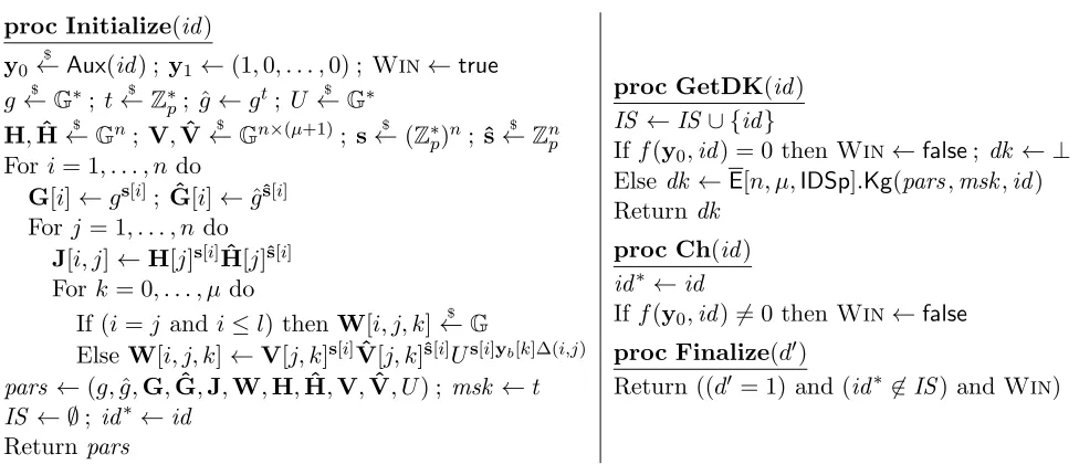
proc Initialize(id) y0
$
←Aux(id) ; y1←(1,0, . . . ,0) ; Win←true
g←$ G∗; t←$ Zp∗; ˆg←gt; U ←$ G∗
H,Hˆ ←$ Gn; V,Vˆ ←$ Gn×(µ+1); s←$ (Z∗p)n;ˆs←$ Znp For i= 1, . . . , n do
G[i]←gs[i]; Gˆ[i]←gˆˆs[i] For j= 1, . . . , n do
J[i, j]←H[j]s[i]Hˆ[j]ˆs[i] Fork= 0, . . . , µ do
If (i=j andi≤l) thenW[i, j, k]←$ G
Else W[i, j, k]←V[j, k]s[i]Vˆ[j, k]ˆs[i]Us[i]yb[k]∆(i,j)
pars ←(g,g,ˆ G,Gˆ,J,W,H,Hˆ,V,Vˆ, U) ;msk ←t
IS ← ∅; id∗ ←id Return pars
proc GetDK(id) IS ←IS ∪ {id}
Iff(y0,id) = 0 thenWin←false; dk ← ⊥ Else dk ←E[n, µ,IDSp].Kg(pars,msk,id) Returndk
proc Ch(id) id∗←id
Iff(y0,id)6= 0 then Win←false proc Finalize(d′)
Return ((d′ = 1) and (id∗ 6∈IS) andWin)
Figure 4: Games RLl,b (0≤l≤nand b∈ {0,1}) associated ton, µ,IDSp,Aux for proof of Lemma 4.2.
4.5 Proof of Lemma 4.2
Consider the games of Figure 4. Game RLl,b makes the diagonal entries of W (namely all the µ+ 1
entries with i = j) random for i ≤ l and otherwise makes them using yb. Game RL0,1 is the same as game RL0 and game RL0,0 is the same as game RLn. Games RLn,0,RLn,1 are identical: both make all diagonal entries of W (meaning, i= j) random, and when i =6 j we have ∆(i, j) = 0 so yb(k) has no
impact on W[i, j, k] in the Else statement. Thus we have Pr[RLA0]−Pr[RLAn] = Pr[RL0A,1]−Pr[RLAn,1]
+ Pr[RLAn,0]−Pr[RLA0,0]
.
We will design adversaries P0, P1 so that Pr[ReCP0
]−Pr[RaCP0
] = 1
n· Pr[RL
A
n,0]−Pr[RLA0,0]
(8) Pr[ReCP1]
−Pr[RaCP1] = 1
n· Pr[RL
A
0,1]−Pr[RLAn,1]
. (9)
Adversary P picks b ← {$ 0,1} and runs Pb. This yields Equation (10). Now we present adversary Pb
When A makes query Initialize(id), adversary Pb begins with
l← {$ 1, . . . , n}; y0 $
←Aux(id) ; y1 ←(1,0, . . . ,0) ; WinA←true; ISA← ∅
(g,g, H,ˆ H,ˆ U,Uˆ, U)←$ Initialize(yb) ; (G,G, S,ˆ Z)
$
←Ch().
Here Pb has called its ownInitializeprocedure with input yb and then called its Chprocedure. Now it
creates parameters pars forA as follows: h,hˆ←$ Zn
p ; v,vˆ
$
←Znp×(µ+1);s←$ (Z∗
p)n;ˆs
$
←Zn
p
For i= 1, . . . , n do
If (i=l) thenH[i]←H; Hˆ[i]←Hˆ ; G[i]←G;Gˆ[i]←Gˆ
If (i6=l) thenH[i]←gh[i];Hˆ[i]←gˆˆh[i]
; G[i]←gs[i]; Gˆ[i]←gˆˆs[i] Fork= 0, . . . , µ do
If (i=l) then V[i, k]←U[k] ; Vˆ[i, k]←Uˆ[k] If (i6=l) then V[i, k]←gv[i,k]; Vˆ[i, k]←gˆˆv[i,k] For i= 1, . . . , n do
Forj= 1, . . . , n do
If (i=land j=i) thenJ[i, j]←S
If (i=land j6=i) thenJ[i, j]←Gh[j]Gˆhˆ[j]
If (i6=l) then J[i, j]←H[j]s[i]Hˆ[j]ˆs[i] For k= 0, . . . , µdo
If (i=j and i≤l−1) thenW[i, j, k]←$ G If (i=j and i=l) thenW[i, j, k]←Z[k] Else W[i, j, k]←V[j, k]s[i]Vˆ[j, k]ˆs[i]Us[i]yb[k]∆(i,j)
pars ←(g,g,ˆ G,Gˆ,J,W,H,Hˆ,V,Vˆ, U) It returns pars to A.
When adversary A makes queryGetDK(id), adversaryPb proceeds as follows. In this code,GetDK is
Pb’s own oracle:
ISA←ISA∪ {id}
If f(y0,id) = 0 thenWinA←false; dk ← ⊥
Else
(D1, D2, D3, D4) $
←GetDK(id) r′ $
←(Z∗p)n;ˆr′ ←$ Znp Fori= 1, . . . , n do
If i=l then (D1[i],D2[i],D3[i],D4[i])←(D1, D2, D3, D4) Else
D1[i]← H(V[i,·],id)r
′[i]
H[i]ˆr′[i]
; D2[i]←gf(vˆ,id)r
′[i] ghˆ[i]ˆr[i] D3[i]←g−r
′[i]
; D4[i]←g−ˆr
′[i]
dk ←(D1,D2,D3,D4)
It returns dk to A. Notice that Pb’s invocation of GetDKwill never return ⊥. In the case b= 1 this is
true becausef(y1,·) = 1= 0. In the case6 b= 0 it is true because the casef(y0,id) = 0 was excluded by the If statement. To justify the above simulation, define r,ˆrby r[i] =r′[i]/t andˆr[i] =ˆr′[i]/t for i6=l
and r[l],ˆr[l] as the randomness underlying (D1, D2, D3, D4). Then think of r,ˆr as the randomness used by the real key generation algorithm. Here t is the secret key, so that ˆg=gt.
When adversary A makes query Ch(id), adversary Pb proceeds as follows:
id∗ ←id
proc Initialize(id) // RL0 y0
$
←Aux(id) ; y1←(1,0, . . . ,0) (pars,msk)←$ E[n, µ,IDSp].Pg(y1) IS ← ∅; id∗←id ; Win←true Return pars
proc Initialize(id) // RLn
y0 $
←Aux(id) ; y1←(1,0, . . . ,0) (pars,msk)←$ E[n, µ,IDSp].Pg(y0) IS ← ∅; id∗←id ; Win←true Return pars
proc GetDK(id) // RL0,RLn
IS ←IS ∪ {id}
Iff(y0,id) = 0 thenWin←false; dk ← ⊥ Else dk ←E[n, µ,IDSp].Kg(pars,msk,id) Return dk
proc Ch(id) // RL0,RLn
id∗←id
Iff(y0,id)6= 0 thenWin←false proc Finalize(d′) // RL0,RLn
Return ((d′= 1) and (id∗ 6∈IS) andWin)
Figure 5: Games RL0,RLn(“Real-to-Losssy”) associated ton, µ,IDSp⊆Zµp and auxiliary input generator
algorithm Aux.
Finally,Ahalts with outputd′. AdversariesP0, P1 compute their output differently. AdversaryP1returns 1 if
(d′ = 1) andid∗ 6∈ISAand WinA
and 0 otherwise. Adversary P0 does the opposite, returning 0 if the above condition is true and 1 otherwise. We obtain Equations (8), (9) as follows:
Pr[ReCP1]
−Pr[RaCP1] = 1
n
n
X
l=1
Pr[RLAl−1,1]−Pr[RLAl,1] = Pr[RLA0,1]−Pr[RLAn,1]
Pr[ReCP0]
−Pr[RaCP0] = 1
n
n
X
l=1
(1−Pr[RLAl−1,0])−(1−Pr[RLAl,0])
= 1
n
n
X
l=1
Pr[RLAl,0]−Pr[RLAl−1,0] = Pr[RLAn,0]−Pr[RLA0,0]. 4.6 Real-to-lossy lemma
Consider games RL0,RLn of Figure 5 associated to some choice of n, µ,IDSp⊆ Zµp and auxiliary input
generatorAuxforE[n, µ,IDSp]. The latter is an algorithm that takes input an identity inIDSpand returns an auxiliary input in Zµp+1. Game RL0 obtains an auxiliary input y0 via Aux but generates parameters exactly as E[n, µ,IDSp].Pg with the real auxiliary input y1. The game will return true under the same condition as game Real but additionally requiring that f(y0,id) 6= 0 for all GetDK(id) queries and
f(y0,id) = 0 for the Ch(id) query. Game RLn generates parameters with the auxiliary input provided
by Auxbut is otherwise identical to game RL0. The following lemma says it is hard to distinguish these games. We will apply this by definingAux in such a way that its outputy0 results in a lossy setup. The proof of the following is in Section 4.5.
Lemma 4.2 Let n, µ ≥ 1 be integers and IDSp ⊆ Zµp. Let Aux be an auxiliary input generator for E[n, µ,IDSp]and A an adversary. Then there is an adversary P such that
Pr[RLA0]−Pr[RLAn] ≤ 2n· Pr
ReCP
−Pr
RaCP
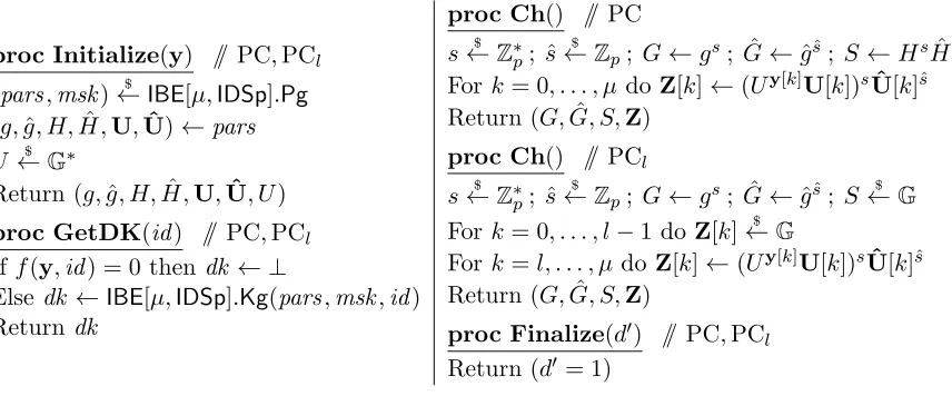
proc Initialize(y) // PC,PCl
(pars,msk)←$ IBE[µ,IDSp].Pg (g,g, H,ˆ H,ˆ U,Uˆ)←pars
U ←$ G∗
Return (g,g, H,ˆ H,ˆ U,Uˆ, U) proc GetDK(id) // PC,PCl
Iff(y,id) = 0 thendk ← ⊥
Else dk ←IBE[µ,IDSp].Kg(pars,msk,id) Returndk
proc Ch() // PC
s←$ Z∗
p; ˆs
$
←Zp; G←gs; ˆG←gˆˆs; S←HsHˆˆs Fork= 0, . . . , µ doZ[k]←(Uy[k]U[k])sUˆ[k]ˆs
Return (G,G, S,ˆ Z) proc Ch() // PCl
s←$ Z∗
p; ˆs
$
←Zp; G←gs; ˆG←gˆˆs; S←$ G Fork= 0, . . . , l−1 doZ[k]←$ G
Fork=l, . . . , µ do Z[k]←(Uy[k]U[k])sUˆ[k]ˆs
Return (G,G, S,ˆ Z)
proc Finalize(d′) // PC,PCl
Return (d′ = 1)
Figure 6: Games PC,PCl (0≤l≤µ+ 1) associated toIDSp⊆Zµp+1 for the proof of Lemma 4.1.
The running time of P is that of A plus some overhead. IfA is selective-id then so isP.
The last statement allows us to use the lemma in both the selective-id and adaptive-id cases.
4.7 Proof of Lemma 4.1
Consider the games of Figure 6. Game PC is the same as game ReC. Game PCl (0 ≤l≤µ+ 1) makes
S random and also makes the firstl−1 entries of Z random and the rest real. Thus PCµ+1 is the same as RaC. We will design adversaries B1, B2 so that
Advdlin(B1) = Pr[PCP]−Pr[PCP0] (11)
Advdlin(B2) = 1
µ+ 1 Pr[PC
P
0]−Pr[PCPµ+1]
(12) AdversaryB will runB1 with probability 1/(µ+ 2) andB2 with probability (µ+ 1)/(µ+ 2). This yields Equation (7).
On input (g,ˆg, gs,ˆgsˆ, H, T) whereT is eitherHs+ˆsor random, adversaryB
1 runs adversaryP, responding to its oracle queries as follows. When P makes queryInitialize(y), adversary B1 lets
u,uˆ←$ Zµp+1; u, v ←$ Zp; ˆH ←Hˆgv; U ←gˆu
For k= 0, . . . , µdo U[k]←U−y[k]gu[k];Uˆ[k]←ˆgˆu[k]
It returns (g,ˆg, H,H,ˆ U,Uˆ, U) to P. WhenP makes its (single)Ch() query, adversaryB1 lets
S ←Tˆgvsˆ
For k= 0, . . . , µdo Z[k]←gsu[k]gˆˆsˆu[k]
It returns (gs,gˆsˆ, S,Z) to P. Notice that for 0≤k≤µ
Z[k] =gsu[k]gˆˆsˆu[k]= (Uy[k]−y[k]gu[k])sgˆˆsˆu[k]= (Uy[k]U[k])sUˆ[k]sˆ.
Also if T =Hs+ˆs thenS=Tgˆvsˆ=Hs(Hˆgv)ˆs=HsHˆˆsas in PC while ifT is random, so is S, as in PC0. When P makes query GetDK(id), adversary B1 does the following:
Else
r′,rˆ′ ←$ Zp
D1 ←g−f(y,id)ur
′
gf(u,id)r′
H−f(u,id)ˆr′/f(y,id)
;D2 ←gf(ˆu,id)r
′
H−f(u,id)ˆr′/f(y,id)ˆ Hurˆ′ D3 ←Hrˆ′/f(y,id)g−r′; D4←gˆ−uˆr′; dk ←(D1, D2, D3, D4)
It returns dk to P. We now show this key is properly distributed. Leth be such that H=gh and let
r = r′
t − hrˆ′
tf(y,id) modp and rˆ = urˆ
′ modp .
Since t, f(y, uid) are non-zero modulo p and r′,rˆ′ are random, r,rˆ are random as well. The following computes the correct secret key components with the above randomness and shows that they are the ones of the simulation:
H(U,id)trHtrˆ = U[0]trQµ
k=1U[k]id[k]tr
Htˆr
= U−y[0]trgu[0]trQµ
k=1U−
y[k]id[k]trgu[k]id[k]trHtrˆ
= U−f(y,id)trgf(u,id)trHtˆr
= U−f(y,id)(r′−hˆr′/f(y,id))
gf(u,id)(r′−hrˆ′/f(y,id)) Htuˆr′
= ˆg−huˆr′g−f(y,id)ur′gf(u,id)r′g−f(u,id)hˆr′/f(y,id)ghturˆ′
= g−f(y,id)ur′gf(u,id)r′H−f(u,id)ˆr′/f(y,id) = D1
H(Uˆ,id)rHˆrˆ = Uˆ[0]rQµ
k=1Uˆ[k]id[k]r
ˆ
Hrˆ = ˆguˆ[0]rQµ
k=1gˆuˆ[k]id[k]r
ˆ
Hrˆ
= ˆgf(ˆu,id)rHˆrˆ = gf(ˆu,id)trHˆrˆ
= gf(ˆu,id)(r′−hˆr′/f(y,id))Hˆurˆ′ = gf(ˆu,id)r′H−f(u,id)ˆr′/f(y,id)Hˆuˆr′ = D2
g−tr = ghˆr′/f(y,id)−r′ = Hrˆ′/f(y,id)g−r′ = D3
g−trˆ = g−turˆ′ = ˆg−urˆ′ = D4.
Finally adversary P outputsd′. Adversary B1 also outputs d′, so we have Equation (11).
On input (g,g, gˆ s,gˆsˆ,U , Tˆ ) whereT is either ˆUs+ˆsor random, adversaryB2runs adversaryP, responding to its oracle queries as follows. When P makes queryInitialize(y), adversary B1 lets
l← {$ 0, . . . , µ}; u,uˆ←$ Zµp+1; u, h,hˆ←$ Zp; H←gˆh; ˆH ←ˆgˆh; U ←gu For k= 0, . . . , µdo U[k]←Uˆ∆(l,k)gu[k];Uˆ[k]←Uˆ∆(l,k)gˆuˆ[k]
It returns (g,ˆg, H,H,ˆ U,Uˆ, U) to P. WhenP makes its (single)Ch() query, adversaryB2 lets
S ←$ G
For k= 0, . . . , l−1 do Z[k]←$ G
For k=l, . . . , µdo Z[k]←(gs)uy[k]+u[k](ˆgˆs)ˆu[k]T∆(l,k) It returns (gs,gˆsˆ, S,Z) to P. Notice that for l+ 1≤k≤µ
Z[k] = (gs)uy[k]+u[k](ˆgsˆ)uˆ[k]=Usy[k]U[k]sUˆ[k]sˆ= (Uy[k]U[k])sUˆ[k]ˆs.
If T = ˆUs+ˆs then
Z[l] = (gs)uy[l]+u[l](ˆgsˆ)ˆu[l]T =Usy[l]( ˆU−1U[l])s( ˆU−1Uˆ[l])sˆUˆsUˆˆs= (Uy[l]U[l])sUˆ[l]sˆ
If f(y,id) = 0 thendk ← ⊥ Else
r,rˆ′ ←$ Zp
D1 ←gˆf(u,id)rgˆhrˆ′; D2←gf(u,id)rUˆid[l]rgˆhrˆ′Uˆ−ˆhid[l]r/h
D3 ←gˆ−r; D4 ←Uˆid[l]r/hg−rˆ
′
; dk ←(D1, D2, D3, D4)
It returns dk to P. We now show this key is properly distributed. Let ˆu be such that ˆU =guˆ and let ˆ
r = rˆ′
t −
id[l]ˆur
th modp .
Since t is non-zero modulop and ˆr′ is random, ˆr is random as well. The following computes the correct secret key components with the above randomness and shows that they are the ones of the simulation:
H(U,id)trHtˆr = U[0]trQµ
k=1U[k]id[k]tr
Htˆr
= gu[0]trQµ
k=1Uˆ
id[k]tr∆(l,k)gu[k]id[k]trgˆhtˆr
= gf(u,id)trUˆid[l]trˆghtˆr = gf(u,id)trUˆid[l]trgˆh(ˆr′−id[l]ˆur/h)
= ˆgf(u,id)rUˆid[l]trgˆhˆr′ˆg−id[l]ˆur = ˆgf(u,id)rgid[l]ˆurtgˆhˆr′ˆg−id[l]ˆur
= ˆgf(u,id)rˆghˆr′ = D1
H(Uˆ,id)rHˆˆr = Uˆ[0]rQµ
k=1Uˆ[k]id[k]r
ˆ
Hrˆ = guˆ[0]rQµ
k=1Uˆid[k]r∆(l,k)guˆ[k]id[k]r
ˆ
gˆhrˆ
= gf(ˆu,id)rUˆid[l]rgtˆhˆr = gf(ˆu,id)rUˆid[l]rgˆh(ˆr′−id[l]ˆur/h)
= gf(ˆu,id)rUˆid[l]rgˆhrˆ′g−ˆhid[l]ˆur/h = gf(u,id)rUˆid[l]rghˆrˆ′Uˆ−hˆid[l]r/h = D2
g−tr = ˆg−r = D3
g−trˆ = gurˆ id[l]/h−rˆ′ = ˆUid[l]r/hg−rˆ′ = D4 . Finally adversary P outputsd′. Adversary B2 also outputs d′. So
Advdlin(B2) = 1
µ+ 1
µ
X
l=0
Pr[PCPl ]−Pr[PCPl+1]
= 1
µ+ 1Pr[PC
P
0]−Pr[PCPµ+1] and we have Equation (12).
4.8 Selective-id security
We consider IBTDF F[n,1,Zp], the instance of our construction with µ = 1 andIDSp = Zp. We show that this IBTDF is selective-id δ-lossy for δ = 1, meaning fully selective-id lossy, and hence selective-id one-way. To do this we define a sibling LF[n,1,Zp]. It preserves the key-generation, evaluation and inversion algorithms of F[n,1,Zp] and alters parameter generation to
Algorithm LF[n,1,Zp].Pg(id)
y←(−id,1) ; (pars,msk)←$ E[n,1,Zp].Pg(y) ; Return (pars,msk)
Theorem 4.3 Let n >2 lg(p) and let ℓ =n−2 lg(p). Let F = F[n,1,Zp] be the IBTDF associated by our construction to parameters n, µ = 1 and IDSp=Zp. Let LF =LF[n,1,Zp] be the sibling associated to it as above. Let δ = 1 and let be A a selective-id adversary. Then there is an adversary B such that
AdvδF-,LFlos,ℓ(A) ≤ 2n(µ+ 2)·Advdlin(B). (13)
The running time of B is that of A plus overhead.
Proof of Theorem 4.3: On input id, let algorithm Aux return (−id,1). Let RL0,RLn be the games
of Figure 5 with µ= 1,IDSp=Zp and thisAux. Then we claim Pr
RealAF
= Pr
RLA0
and Pr
LossyAF,LF,ℓ
= Pr
RLAn
. (14)
To justify this let id∗ be the identity queried by A to both Initialize and Ch. (These queries are the same because A is selective-id.) Then y0 = (−id∗,1) so f(y0,id) = id −id∗. This is 0 iff id = id∗. This means that the conjunct (id∗ 6∈IS)∧Win is always true. The claim of Equation (14) is now true because game RL0generates parameters with the real auxiliary inputy1 = (1,0) ∈Z2pthat, viaE[n,1,Zp],
defines F. However game RLn generates parameters with auxiliary input y0. Since f(y0,id∗) = 0, the dependency of C3[j] on x[j] in Equation (5) vanishes when id = id∗. Examing equations (3), (4), (5), (6), we now see that with pars fixed, the values hs, xi,hˆs, xi determine the ciphertext (C1, C2,C3,C4). Thus there are at most p2 possible ciphertexts whenid =id∗, and 2n possible inputs. This means that
λ(F.Ev(pars,id∗,·)) ≥n−lg(p2) = ℓ, which justifies the second claim of Equation (14). Recalling that
δ = 1, Equation (13) follows from Equation (1), Equation (14), Lemma 4.2 and Lemma 4.1.
4.9 Adaptive-id Security
We consider IBTDF F[n, µ,{0,1}µ], the instance of our construction withIDSp={0,1}µ ⊂Zµ
p. We show
that this IBTDF is adaptive-id δ-lossy for δ = (4(µ+ 1)Q)−1 where Q is the number of key-derivation queries of the adversary. By Theorem 3.2 this means F[n, µ,{0,1}µ] is adaptive-id one-way. To do this
we define a siblingLFQ[n, µ,{0,1}µ]. It preserves the key-generation, evaluation and inversion algorithms
of F[n, µ,{0,1}µ] and alters parameter generation toLF[n, µ,{0,1}µ].Pg(id) defined via y←Aux; (pars,msk)←$ E[n, µ,{0,1}µ].Pg(y) ; Return (pars,msk).
where algorithm Aux is defined via
y′[0]← {$ 0, . . . ,2Q−1}; ℓ← {$ 0, . . . , µ+ 1}; y[0]←y′[0]−2ℓQ
Fori= 1 toµ doy[i]← {$ 0, . . . ,2Q−1} Return y∈Zµp+1
The following says that our IBTDF is δ-lossy under the DLIN assumption with lossinessℓ=n−2 lg(p). Theorem 4.4 Letn >2 lg(p)and let ℓ=n−2 lg(p). LetF=F[n, µ,{0,1}µ]be the IBTDF associated by
our construction to parameters n, µ and IDSp={0,1}µ. Let A be an adaptive-id adversary that makes a maximal number of Q < p/(3m) queries and let δ = (4(µ+ 1)Q)−1. Let LF=LF
Q[n, µ,{0,1}µ] be the
sibling associated to F, A as above. Then there is an adversary B such that
AdvδF-,LFlos,ℓ(A) ≤ 2n(µ+ 2)·Advdlin(B). (15)
The running time of B is that of A plus O(µ2ρ−1((µQρ)−1)) overhead, where ρ= 12 ·AdvδF-,LFlos,ℓ(A). Proof of Theorem 4.4: Our proof uses a simulation technique due to Waters [62]. We used a slightly improved analysis from [42]. LetQbe the number of queries made byAand let algorithmAuxbe defined as above. Let RL0,RLnbe the games of Figure 5 withIDSp={0,1}µand thisAux. LetE(IS,id∗) denote
the event that when procFinalize(d′) is called in RLA
the probability that E(IS,id∗) happens. In [42, Lemma 6.2], it was shown (using purely combinatorial arguments) that λlow := 4(µ+1)1 Q ≤ η(IS,id∗) ≤ 21Q := λup. Since RLA0 and RealAF are only different when E(IS,id∗) happens, one would like to argue that λlow·PrRealAF
= Pr
RLA0
but this is not true since E(IS,id∗) and RealAF may not be independent. To get rid of this unwanted dependence we consider a modification of RL0 and RLnwhich adds some artificial abort such that in total it always sets
Win ← false with probability around 1−λlow, independent of the view of the adversary. (Since, given IS,id∗, the exact value of η(IS,id∗) cannot be computed efficiently, it needs to be approximated using sampling.) Concretely, games ˆRL0 and ˆRLnare defined as RL0 and RLn, respectively, the only difference
being Finalizewhich is defined as follows. proc Finalize(d′) // ˆRL0,RLˆ n
Compute an approximation η′(IS,id∗) of η(IS,id∗) If η′(IS,id∗)> λ
low then setWin←false with probability 1−λlow/η′(IS,id∗) Return ((d′ = 1) and (id∗ 6∈IS) and Win)
We refer to [42] on details how to compute the approximation η′(IS,id∗). Using [42, Lemma 6.3], one can show that if we use O(µ2ρ−1((µQρ)−1)) samples to compute approximationη′(IS,id∗), then
Pr
RealAF
−λ−low1 ·PrhRLˆ A0 i=ρ. (16)
Setting ρ= 12 ·Pr
RealAF
we obtain
δ·Pr
RealAF
= PrhRLˆ A0 i, (17)
where δ=λlow/2 is as in the theorem statement. As in the proof of Theorem 4.3, we can show that Pr
LossyAF,LF,ℓ
= PrhRLˆ Ani. (18)
Now Equation (15) follows from Equations (1), (17), (18), Lemma 4.2 and (a version incorporating the artificial abort of) Lemma 4.1.
We remark that we could use the proof technique of [12] which avoids the artificial abort but this increases the value of δ, making it dependent on the adversary advantage. The proof technique of [41] could be used to strengthen δ in Theorem 4.4 to O(√mQ)−1 which is close to the optimal valueQ−1.
5
IB-TDFs from Lattices
Here we give a construction of a lossy IB-TDF from lattices, specifically, the LWE assumption. We note that a one-way IB-TDF can already be derived by applying methods from [29, 2] to the LWE-based injective (not identity-based) trapdoor function from [36].
LWE is a particular type of average-case BDD/GapSVP problem. It has been recognized since [50] that GapSVP (and BDD [45]) induces a form of lossiness. So there is folklore that the GPV LWE-based TDF can be made to satisfy some meaningful notion of lossiness (specifically, for an appropriate input distribution, the output does not reveal the entire input statistically) by replacing its normally uniformly random key with an LWE (BDD/GapSVP) instance. However, a full construction and proof according to the standard notion of lossiness (which compares the domain and images sizes of the function) have not yet appeared in the literature, and there are many quantitative issues to address.