Western University Western University
Scholarship@Western
Scholarship@Western
Electronic Thesis and Dissertation Repository
8-1-2019 2:00 PM
Split credibility: A two-dimensional semi-linear credibility model
Split credibility: A two-dimensional semi-linear credibility model
Jingbing QiuThe University of Western Ontario
Supervisor Jiandong Ren
The University of Western Ontario
Graduate Program in Statistics and Actuarial Sciences
A thesis submitted in partial fulfillment of the requirements for the degree in Master of Science © Jingbing Qiu 2019
Follow this and additional works at: https://ir.lib.uwo.ca/etd
Part of the Statistical Models Commons
Recommended Citation Recommended Citation
Qiu, Jingbing, "Split credibility: A two-dimensional semi-linear credibility model" (2019). Electronic Thesis and Dissertation Repository. 6309.
https://ir.lib.uwo.ca/etd/6309
This Dissertation/Thesis is brought to you for free and open access by Scholarship@Western. It has been accepted for inclusion in Electronic Thesis and Dissertation Repository by an authorized administrator of
Abstract
In the thesis, we introduce a two-dimensional semi-linear credibility model, which is an extension of the classical credibility or split credibility models used by practicing actuaries. Our model predicts the future expected losses of a policyholder by considering its historical primary and excess losses. The optimal split point is derived based on the mean squared error criterion. We show when and why splitting a policyholder’s historical losses into primary and excess parts work analytically. In addition, we derived formulas for estimating our model parameters nonparametrically. Finally, we show the application of our model through three examples.
Keywords: Two-dimensional semi-linear credibility model, split credibility, primary and
excess credibility, linear function, mean square error
Summary for Lay Audience
Credibility theory is a set of quantitative tools that allows an insurer to adjust premiums based on policy holders’ past loss experience. The theory features the combination of data with other information, such as the mean loss of policyholders in the same rating class.
In this thesis, we introduce a two-dimensional semi-linear credibility model, which consid-ers policyholdconsid-ers’ small losses and large losses separately. Our model is an extension of the classical credibility or split credibility models used by practicing actuaries.
Acknowlegements
The author gratefully acknowleges the supervisor, Jiandong Ren for his insights and observa-tions. He gave the author detailed and thoughtful comments and suggesobserva-tions. The author also would like to acknowlege friends and loved ones for their support and encouragement. These contributions helped to motivate and substantially improve the thesis.
Contents
Abstract ii
Summary for Lay Audience iii
Acknowlegements iv
List of Figures vii
List of Tables viii
List of Appendices ix
1 Introduction 1
1.1 Limited fluctuation crediblity theory . . . 2
1.2 Greatest accuracy credbility theory . . . 3
1.3 Split credibility . . . 7
1.4 Semi-linear credibility with truncation . . . 9
1.5 Our model . . . 11
2 Two-dimensional semi-linear credibility model 12 2.1 General results . . . 12
2.1.1 The optimalα’s . . . 12
2.1.2 The minimum value of MSE . . . 17
2.1.3 Summary . . . 17
2.2 Split results . . . 18
2.2.1 Properties of credibility . . . 20
2.2.2 The optimal split point . . . 21
2.2.3 Nonparametric estimation . . . 24
2.2.4 The estimators ofµp(θ) andµe(θ) . . . 28
3 Examples 31 3.1 Exponential distribution conditional onΘ . . . 31
3.1.1 Parametric estimation . . . 32
3.1.2 Nonparametric estimation . . . 39
3.2 Poisson distribution conditional onΘ . . . 40
3.3 Mixture of two Exponential distributions conditional onΘ . . . 47
3.3.1 Parametric estimation . . . 48
3.3.2 Nonparametric estimation . . . 53
4 Conclusion 55
Bibliography 56
A Propositions 57
B Formulas of nonparametric estimation 59
C R code of examples 61
Curriculum Vitae 73
List of Figures
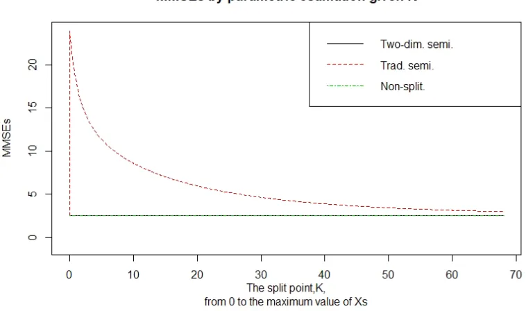
3.1 MMSEs by parametric estimation given K in example1 . . . 40
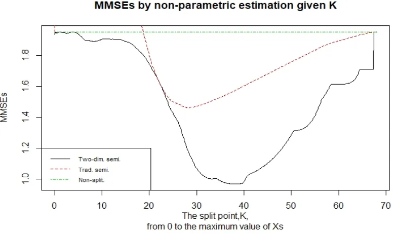
3.2 MMSEs by nonparametric estimation given K in example1 . . . 42
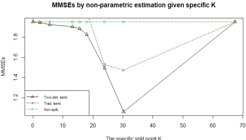
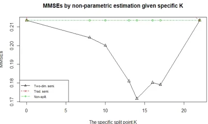
3.3 MMSEs by nonparametric estimation given specific K in example1 . . . 43
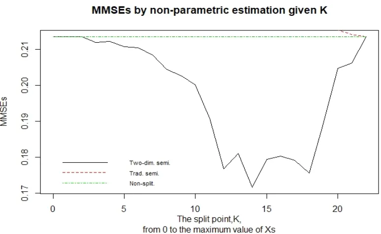
3.4 MMSEs by nonparametric estimation given K in example2 . . . 45
3.5 MMSEs by nonparametric estimation given specific K in example2 . . . 47
3.6 MMSEs by parametric estimation given K in example3 . . . 52
3.7 MMSEs by nonparametric estimation given K in example3 . . . 53
3.8 MMSEs by nonparametric estimation given specific K in example3 . . . 54
List of Tables
2.1 A list of notations . . . 14
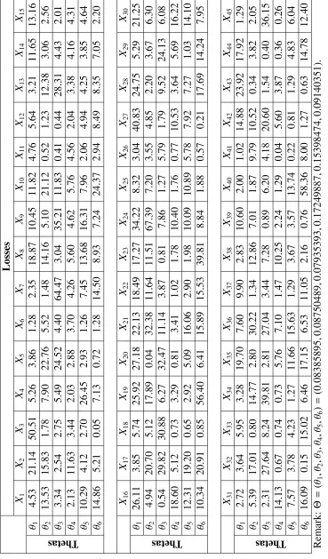
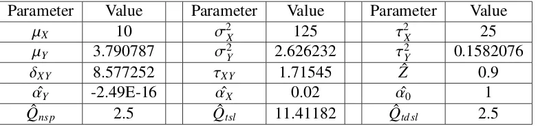
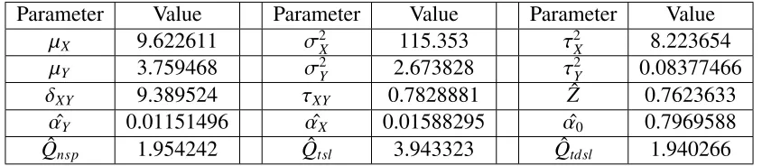
3.1 A set of data from R code in example1 (only two decimals) . . . 33 3.2 The value of parameters by parametric estimation calculated using R in
exam-ple1 (whenK =5) . . . 39 3.3 The value of parameters by nonparametric estimation calculated using R in
example1 (whenK = 5) . . . 41 3.4 A set of data from R code in example2 . . . 46 3.5 A set of data from R code in example3 (only two decimals) . . . 49 3.6 The value of parameters by parametric estimation calculated using R in
exam-ple 3 (whenK = 7.99) . . . 52
B.1 A list of data . . . 59
List of Appendices
Appendix A Propositions . . . 57 Appendix B Formulas of nonparametric estimation . . . 59 Appendix C R code of examples . . . 61
Chapter 1
Introduction
Credibility theory is a quantitative tool that enables us to estimate and adjusts the future pre-mium given a policyholder’s loss experience. For a detailed introduction of credibility theory, readers are referred to Klugman et al. [8]. Assume that the risks are homogeneous, the manual rate is designed to reflect the past and future expected experience of the entire rating class. Because the policyholders in a rating class are different, the manual rate can not reflect individ-uals’ actual risk. However, it is important that higher risks should have higher rate and lower risks should have lower rate.
Therefore, the insurer is forced to determine how much of the difference between the pol-icyholder’s own experience and the expected experience is due to random fluctuations as well as how much is due to the fact that the policyholder’s own risk is higher or lower than the average risk. That is, how much credibility does the policyholder’s own experience have? The credibility necessarily depends on the amount of data. The more past information we have on a given policyholder, the more credible the policyholder’s own experience, all other things being equal. In group insurance, the loss experience of larger groups are more credible than that of small groups.
Another use for credibility is in the setting of rates for classification systems. For example, there may be many occupational classes in workers compensation insurance, some of which may provide very little data. In order to accurately estimate the expected cost for insuring these classes, limited empirical data can be combined with other information, such as past rates and so on.
From a statistical point of view, if loss experience data from an insured or group of insureds is avaiable, we should use the sample mean or some other unbiased estimator to determine the premium. But the results in credibility theory show that it is optimal to give only partial weight to this experience and give the remaining weight to an estimator produced from other information. For details, readers are referred to Klugman et al. [8].
Credibility theory is an approach to combine the manual rate with the policyholder’s own loss experience, so that future premium will reflect the future losses accurately. In this chapter, we firstly introducelimited fluctuation crediblity theory, a subject developed in the early part of the twentieth century. The theory provides an approach to assign full or partial credibility to a policyholder’s experience. Then, we will introducegreatest accuracy credbility theory, which was formalized by B¨uhlmann [1]. The simplest model of B¨uhlmann [1] is introduced in this section and will be our assumption in the thesis. Besides that, we will introduce an improved
2 Chapter1. Introduction
model that developed by B¨uhlmann and Straub [3], after the simplest B¨uhlmann model. Then, we will introduce split credibility which is the research object of the thesis. We firstly introduce semi-linear credibility with truncation (referred to B¨uhlmann et al. [4]). Then we propose our two-dimensional semi-linear credibility model.
The thesis is organised as follows. In chapter 2, we discuss our two-dimensional semi-linear credibility model and also discuss the nonparametric estimation method associated with our model. In chapter 3, we show the application of the model with three examples. Chapter 4 concludes the thesis.
1.1
Limited fluctuation crediblity theory
Limited fluctuation crediblity theory is an approach to determine whether we should assign full credibility on the policyholder’s own past experience or not and decide to assign partial credibility if full credibility is inappropriate. Suppose that a policyholder has experienced Xj
claims or losses in past experience period j, where j∈ {1,2,3,· · · ,n}. Suppose thatE(Xj)= ξ
and Var(Xj) = σ2 for all j. The past experience may be summarized by the average ¯X =
1
n
Pn
j=1Xj. Notice thatE( ¯X)=ξand if theXj are independent,Var( ¯X)= σ 2 n.
The insurer’s goal is to determine the value ofξ. One way is to ignore the past experience and simply charge M, a value obtained from experience on other similar but not identical policyholders, which is often called the manual premium. Another way is to ignore M and charge ¯X, which is full credibility. A third way is to choose some combination of M and ¯X, which is partial credibility.
For full credibility, we use statistical method to decide whether the losses are stable or not. That is, selecting two numbersr > 0 and 0 < p < 1 (with r close to 0 and pclose to 1) and assigning full credibility if
Pr(−rξ≤ X¯ −ξ≤ rξ)≥ p. (1.1) Restate (1.1) as
Pr
¯ X−ξ
σ/√n
≤ rξ √
n σ
≥ p. (1.2)
Letypbe defined by
yp =inf y
Pr
¯ X−ξ
σ/√n
≤y
≥ p
. (1.3)
Then the condition for full credibility is
rξ√n
σ ≥yp. (1.4)
Rewrite (1.4) as
σ ξ ≤
r
yp
√
n=
s
n λ0
1.2. Greatest accuracy credbility theory 3
whereλ0 =(yp/r)2. If the Xjare independent, we can rewrite (1.5) as
Var( ¯X)= σ
2
n ≤ ξ2
λ0
. (1.6)
Alternatively, solving (1.5) forngives the number of exposure units required for full cred-ibility, namely,
n≥ λ0
σ ξ
2
. (1.7)
For details, readers are referred to Klugman et al. [8]. Thus, we can get the condition of sample size which meets the standard for full credibility.
If full credibility above is inappropriate, we consider partial credibility which contains the past experience ¯Xin the net premium as well as the externally obtained mean,M. Then we get the formula of credibility premium,
Pc =ZX¯ +(1−Z)M, (1.8)
where the credibility factorZ ∈[0,1] needs to be chosen. The theoretical method on the basis of a statistical model to determine the optimal Z will be presented in next section. Another method is based on the same idea as full credibility. We see from (1.6) that there is no assurance that the variance of X will be small enough. However, it is possible to control the variance of the credibility premium,Pc, as follows:
ξ2
λ0
= Var(Pc)
= VarhZX¯ +(1−Z)Mi
= Z2Var( ¯X)
= Z2σ
2
n.
Thus,Z =(ξ/σ)√n/λ0. Due toZ ∈[0,1], we have that
Z =min
ξ σ
s
n λ0
,1
. (1.9)
1.2
Greatest accuracy credbility theory
B¨uhlmann [1] introduced a model-based approach to solve the credibility problem. Sup-pose that we have the past claims for a particular policyholder with n exposure units, X = (X1,X2,· · · ,Xn)T, and a manual rate µ(it is the same as M above) applicable to this
4 Chapter1. Introduction
is discussed in Klugman et al. [8]. But here we do not discuss the Bayesian methodology in detail, and focus on the B¨uhlmann model (the simplest credibility model).
Under the B¨uhlmann model, for each policyholder, past losses X1, . . . ,Xn are assumed to
have the same mean and variance and are i.i.d. conditional onΘ. Assume thatΘis a random variable which is the risk parameter associated with the policyholder. Define
µ(θ) = E(Xj|Θ = θ),
v(θ) = Var(Xj|Θ =θ),
µ = E(µ(Θ)), v = E(v(Θ)),
a = Var[µ(Θ)].
We are interested in setting a rate to coverXn+1. Define
µn+1(θ) = E(Xn+1|Θ =θ),
µn+1 = E(µn+1(Θ)).
Now, we can calculate the unconditional mean and variance ofXj as well as ¯X as follows,
E(Xj)= E[E(Xj|Θ)]= E[µ(Θ)]= µ= E( ¯X),
and
Var(Xj) = E[Var(Xj|Θ)]+Var[E(Xj|Θ)]
= E[v(Θ)]+Var[µ(Θ)]
= v+a,
and
Var( ¯X) = E[Var( ¯X|Θ)]+Var[E( ¯X|Θ)]
= E
v(Θ)
n
+Var[µ(Θ)]
= v
n+a.
Because the losses are i.i.d. conditional onΘ, the unconditional mean and variance ofXn+1
are the same asXj’s. That is,
E(Xn+1)= E[E(Xn+1|Θ)]= E[µn+1(Θ)]= E[µ(Θ)]= µ= µn+1,
and
Var(Xn+1) = E[Var(Xn+1|Θ)]+Var[E(Xn+1|Θ)] = E[v(Θ)]+Var[µ(Θ)]
1.2. Greatest accuracy credbility theory 5
B¨uhlmann [1] suggested a linear function of past loss data to estimate a policyholder’s expected loss next yearµn+1(θ). Thus, the credibility premium is
Pc =α0+
n
X
j=1
αjXj, (1.10)
whereα0, α1,· · · , αnare parameters that are needed to be chosen. Hence, we choose the
opti-malα’s to minimize mean squared error(MSE), which is
Q = E
(
µn+1(Θ)−Pc]2
)
(1.11)
= E
(
µn+1(Θ)−α0−
n
X
j=1
αjXj
2)
. (1.12)
Thus, by taking derivatives with regard toα’s in (1.12), it can be shown that the credibility premium is given by
Pc =µdX(θ) = αˆ0+
n
X
j=1
ˆ
αjXj (1.13)
= ZˆX¯ +(1−Zˆ)µ, (1.14)
where
ˆ Z = n
n+k (1.15)
and
k = v a=
E[Var(Xj|Θ)]
Var[E(Xj|Θ)]
(1.16)
and ˆα0is the optimalα0and ˆαjis the optimalαj for all jand ˆZis the optimal credibility factor,
6 Chapter1. Introduction
The minimum mean squared error(MMSE) in the B¨uhlmann model is
ˆ
Q = E
(
µn+1(Θ)−αˆ0−
n
X
j=1
ˆ αjXj
2)
= E
(
µn+1(Θ)−ZˆX¯ −(1−Zˆ)µ 2)
= E
µn+1(Θ)2+ h
ˆ
ZX¯ +(1−Zˆ)µi2−2Xn+1 h
ˆ
ZX¯ +(1−Zˆ)µi
= Enµn+1(Θ)2+Zˆ2X¯2+(1−Zˆ)2µ2+2 ˆZ(1−Xˆ)µX¯ −2 ˆZXn+1X¯ −2(1−Zˆ)µXn+1 o
= E(µn+1(Θ)2)+Zˆ2E( ¯X2)+(1−Zˆ)2µ2+2 ˆZ(1−Xˆ)µ2−2 ˆZE(Xn+1X¯)−2(1−Zˆ)µ2 = Var(µn+1(Θ))+E(µn+1(Θ))2+Zˆ2
Var( ¯X)+E( ¯X)2−2 ˆZEhE(Xn+1X¯|Θ)
i
−(1−Zˆ)2µ2
= a+µ2+Zˆ2
v
n+a+µ
2
−2 ˆZEhE(Xn+1Θ)E( ¯X|Θ)
i
−(1−Zˆ)2µ2
= a+µ2+Zˆ2
v
n+a+µ
2
−2 ˆZE[µ(Θ)2]−(1−Zˆ)2µ2
= a+µ2+Zˆ2
v
n+a+µ
2
−2 ˆZVar(µ(Θ))+E(µ(Θ))2−(1−Zˆ)2µ2
= a+µ2+Zˆ2
v
n+a+µ
2
−2 ˆZ(a+µ2)−(1−Zˆ)2µ2
= Zˆ2v
n+(a+µ
2
)(1−Zˆ)2−(1−Zˆ)2µ2
= Zˆ2v
n+(1−Zˆ)
2 a = na
na+v
2 v n+ v
na+v
2 a
= va(na+v)
(v+na)2
= va
v+na. (1.17)
However, the B¨uhlmann model does not allow for variations in exposure or size. Therefore, the B¨uhlmann-Straub model is presented in B¨uhlmann and Straub [3] to correct the problem. The difference between the B¨uhlmann-Straub model and the B¨uhlmann model is the condi-tional variances. The condicondi-tional variances is assumed to be
Var(Xj|Θ = θ)=
v(θ)
mj
, (1.18)
wheremj is a known constant measuring exposure. This model would be appropriate if each
1.3. Split credibility 7
µ(θ) and variancev(θ). Therefore, the unconditional variance ofXjbecomes
Var(Xj) = E[Var(Xj|Θ)]+Var[E(Xj|Θ)]
= E
v(Θ)
mj
+Var[µ(Θ)]
= v
mj
+a.
To obtain the new credibility premium (1.10), we should take derivatives with regard toα’s in (1.12) again. Define
m=m1+m2+· · ·+mn
to be the total exposure. Then, the credibility premium (1.10) becomes
Pc = µdX(θ) = αˆ0+
n
X
j=1
ˆ
αjXj =ZˆX¯ +(1−Zˆ)µ, (1.19)
where
ˆ
Z = m
m+k (1.20)
wherek =v/afrom (1.16) and
¯ X=
n
X
j=1
mj
mXj. (1.21)
For details, readers are referred to Klugman et al. [8]. They are a simple introduction for traditional credibility theory. From now on, we will discuss the split credibility.
1.3
Split credibility
National Council on Compensation Insurance (NCCI) [10] introduced that NCCI’s Experience Rating Plan Manual for Workers Compensation and Employers Liability Insurance (Plan) was an integral part of determining the cost of workers compensation. This is a way to customize insurance costs based on the characteristics of the employer. It provides employers with the incentive to manage their own expenses through measurable and meaningful cost-saving pro-grams.
However, very large losses including the entire portion of the claim beyond a certain level in the experience period reduces the predictive ability of the Plan. Although very large losses are less likely to occur and are seen as more fortuitous than smaller claims, we should reduce cred-ibility of them for making accurate estimates of future premium. Hence, the split credcred-ibility is presented.
8 Chapter1. Introduction
reflects severity. For individual claims below the split point, the entire amount is primary loss and the excess loss is 0.
Robbin [11] introduced that the Experience Rating Plan for Workers Compensation with a primary-excess split promulgated by the NCCI made the actual losses, denoted byX, divided into primary losses, denoted byXp, and excess losses, denoted byXe. That is,
X = Xp+Xe, (1.22)
where
Xp= min(X,K) and Xe = X−Xp. (1.23)
This plan estimates the future losses by adding together the credibility-weighted estimates of primary and excess losses separately. That is,
Pc = M+ZpX¯p+ZeX¯e (1.24)
where Pc is estimator of the future losses, M = (1−Zp)E(Xp)+ (1−Ze)E(Xe) as well asZp
and Ze are constant to be determined, which are credibility factors. The difference between
the conventional non-split credibility and two split credibility is clear by comparing (1.8) and (1.24).
Robbin [11] assumed that the distributions ofXpandXewere dependent on a risk parameter,
Θ. Define
µp(Θ) = E(Xp|Θ), µe(Θ)= E(Xe|Θ),
vp(Θ) = Var(Xp|Θ), ve(Θ)=Var(Xe|Θ),
µp = E(µp(Θ)), µe =E(µe(Θ)),
vp = E(vp(Θ)), ve = E(ve(Θ)),
ap = Var[µp(Θ)], ae = Var[µe(Θ)],
C(Θ) = Cov(Xp(Θ),Xe(Θ)), ρ= E(C(Θ)),
λp = vp+ap, λe =ve+ae,
π = Cov(µp(Θ), µe(Θ)), κ=ρ+π.
In the above,ρis the process covariance andπis the parameter covariance. The MSE is
Q= E
(
ZpXp+(1−Zp)µp−µp(Θ)+ZeXe+(1−Ze)µe−µp(Θ)
2)
. (1.25)
whereµn+1(Θ)=µ(Θ)=µp(Θ)+µe(Θ).
By taking derivatives with regard toZpandZeseparately in (1.25) and setting them to zero,
the credibility premium is
Pc =µdX(θ)=ZˆpX¯p+(1−Zˆp)µp+ZˆeX¯e+(1−Zˆe)µe, (1.26)
where
ˆ Zp =
λe(ap+π)−κ(ae+π)
D , (1.27)
ˆ Ze =
λp(ae+π)−κ(ap+π)
1.4. Semi-linear credibility with truncation 9
and
D=λpλe−κ2. (1.29)
Hence, the MMSE is
ˆ
Q = E
(
ZpXp+(1−Zp)µp−µp(Θ)+ZeXe+(1−Ze)µe−µp(Θ)
2)
(1.30)
= (ap+π)(1−Zˆp)+(ae+π)(1−Zˆe). (1.31)
For details, readers are referred to Robbin [11].
In Robbin [11], the MSE was regarded as a criterion for optimization. If the MMSE in split credibility would be less than the MMSE in non-split credibility, then the split method should be better than the non-split way. After considering the correlation betweenXpandXe, Robbin
[11] derived the optimal split credibility of each loss by the least squares method and showed when split in effective. However, under collective risk model (CRM), the following situations may make the split ineffective:
1. Inversion: The optimal excess credibility is bigger than the optimal primary credibility. 2. Out of range: One of the optimal split credibilities is beyond 100% or negative.
In fact, Gillam [6][7] showed that there were many empirical evidences for the practicality of split credibility. Why the situations above never happened among those evidences? We find that a pivotal assumption in Gillam [6] is that primary and excess losses are uncorrelated. In addition, the optimal split credibility factors, ˆZpand ˆZe, given by Gillam [6] are different from
Robbin [11]’s. However, we find that they will be same if both the process covariance and parameter covariance are zero in Robbin [11].
As we all know, it is not possible that the process covariance and parameter covariance both become zero becauseXpandXemust exit a correlation because they are from one same X. So
the assumption in Gillam [6] should not be satisfied in reality. This means that we should not ignore the covariances between the primary and excess losses.
1.4
Semi-linear credibility with truncation
B¨uhlmann et al. [2] assumed that the claims(losses) were from two different sources: ordinary claim with density Do(X|Θ) with probability 1−πand excess claim with density De(X) with
probabilityπ. Then, the density function of claims, fΘ(X), is given by
fΘ(X)=(1−π)Do(X|Θ)+πDe(X) (1.32)
To estimate the future premium, we can use Equation (1.13) as before and minimize the MSE (1.11) to get the optimal parameters. However, B¨uhlmann et al. [2] gave us a new way to estimate the future premium. That is,
Pc =a+b n
X
j=1
10 Chapter1. Introduction
wherea,bandM should be chosen by minimizing the MSE,
Q = E
(
E(µ(Θ)|X)−Pc
2)
(1.34)
= E
(
E(µ(Θ)|X)−a−b
n
X
j=1
(Xj∧M)
2)
(1.35)
= E
(
πµe+(1−π)E(µo(Θ)|X)−a−b n
X
j=1
(Xj∧M)
2)
(1.36)
This method is standard credibility technique combined with data trimming, where the parameter, M, is the trimming point.
Notice that in the model, only the ordinary part of the distribution depends on risk parame-ter,Θ. What’s more, we realize that it is a method that keeps only the primary part of the loss distribution. The excess part is ignored. More details about this credibility estimation tech-nique based on transformed data will be seen in B¨uhlmann et al. [4]. It is called semi-linear credibility.
In order to avoid the impact of large claims on the overall credibility premium, B¨uhlmann et al. [4] look for transformations of the data. The credibility estimator is then applied to the transformed data. One approach is to truncate either the aggregate or the individual claims.
In the thesis, the transformed data we assign is given by
Yj = f(Xj)=min(Xj,K) (1.37)
whereKis the truncation point. The new credibility premium is
d
µX(θ)= αˆ0+
n
X
j=1
ˆ
αjYj (1.38)
In B¨uhlmann et al. [4], the semi-linear credibility estimator of µX(θ) in the B¨uhlmann
model, based onYj above, is given by
Pc =b bµ
(K)
X (θ)=µX +
nτXY
nτ2
Y +σ
2
Y
( ¯Y−µY) (1.39)
where
µX = E(µX(Θ)), (1.40)
µY = E(µY(Θ)), (1.41)
τXY = Cov(µX(Θ), µY(Θ)), (1.42)
τ2
Y = Var[µY(Θ)], (1.43)
τ2
X = Var[µX(Θ)], (1.44)
σ2
1.5. Our model 11
The MMSE is given by
ˆ
Q = E
(
b bµ
(K)
X (Θ)−µX(Θ)
2)
(1.46)
= τ2
X −
nτ2XY
nτ2Y+σ2Y (1.47)
We notice that semi-linear credibility includes non-split credibility model because the cred-ibility premium (1.38) would become (1.13) if the optimalK went to infinity.
1.5
Our model
Chapter 2
Two-dimensional semi-linear credibility
model
In this chapter, we look for general results of our model, called two-dimensional semi-linear credibility model, including the optimal coefficients,α’s, and the value of MSE. Then we will make a summary for general results. Next, we will give specific results in split credibility. We will also discuss some properties of credibility in this model and the method for the optimal split point will be presented. Furthermore, nonparametric estimation will be discussed, which is helpful for us to solve the real problems. Finally, we derive the estimators of credibility premium of the primary part and excess part.
In the thesis, we consider the two-dimensional semi-linear credibility model in the simple B¨uhlmann model, that is for each policyholder(conditional on Θ), past losses X1, . . . ,Xn have
the same mean and variance and are i.i.d. conditional onΘ. For details, readers are referred to Klugman et al. [8].
2.1
General results
Based on semi-linear credibility, we have only one transformed dataYj = f(Xj). Now, we add
another transformed data Lj = g(Xj) that is different fromYj into the model. Hence, we get a
new credibility premium(or called estimator). That is,
µX(θ)= α0+
n
X
j=1
αY jYj+ n
X
j=1
αL jLj. (2.1)
2.1.1
The optimal
α
’s
To choose the optimalα’s, we minimize the MSE. That is,
Q= E
(
µn+1(Θ)−α0−
n
X
j=1
αY jYj− n
X
j=1
αL jLj
2)
. (2.2)
2.1. General results 13
Taking derivatives with regard toα’s and setting them to zero yields fori=1, . . . ,n, ∂Q
∂αˆ0
= 0= E
(
2
µn+1(Θ)−αˆ0−
n
X
j=1
ˆ αY jYj−
n
X
j=1
ˆ αL jLj
(−1)
)
, (2.3)
∂Q ∂αˆYi
= 0= E
(
2
µn+1(Θ)−αˆ0−
n
X
j=1
ˆ αY jYj−
n
X
j=1
ˆ αL jLj
(−Yi)
)
, (2.4)
∂Q ∂αˆLi
= 0= E
(
2
µn+1(Θ)−αˆ0−
n
X
j=1
ˆ αY jYj−
n
X
j=1
ˆ αL jLj
(−Li)
)
, (2.5)
where ˆα0is the optimalα0and ˆαYiis the optimalαYiand ˆαLi is the optimalαLifor alli.
Then, expanding them yields
E[µn+1(Θ)] = αˆ0+
n
X
j=1
ˆ
αY jE(Yj)+ n
X
j=1
ˆ
αL jE(Lj), (2.6)
E[µn+1(Θ)Yi] = αˆ0E(Yi)+ n
X
j=1
ˆ
αY jE(YjYi)+ n
X
j=1
ˆ
αL jE(LjYi), (2.7)
E[µn+1(Θ)Li] = αˆ0E(Li)+ n
X
j=1
ˆ
αY jE(YjLi)+ n
X
j=1
ˆ
αL jE(LjLi). (2.8)
The left-hand side of Equation (2.7) can be rewritten as
E[µn+1(Θ)Yi] = EE[µn+1(Θ)Yi|Θ]
= Eµ
n+1(Θ)E[Yi|Θ]
= E
E[Xn+1|Θ]E[Yi|Θ]
= E
E[Xn+1Yi|Θ]
= E[Xn+1Yi],
where the second from the last step follows by independence ofXi andXn+1 conditional onΘ,
which is same as Klugman et al. [8]. Then, Equation (2.7) becomes
E[Xn+1Yi]=αˆ0E(Yi)+ n
X
j=1
ˆ
αY jE(YjYi)+ n
X
j=1
ˆ
αL jE(LjYi). (2.9)
Hence, we also have
E[Xn+1Li]=αˆ0E(Li)+ n
X
j=1
ˆ
αY jE(YjLi)+ n
X
j=1
ˆ
αL jE(LjLi), (2.10)
which is from (2.8) and whose reason is followed by above.
Besides, the left-hand side of Equation (2.6) can be rewritten as
14 Chapter2. Two-dimensional semi-linear credibility model
Hence, we rewrite Equation (2.6) as
E[Xn+1]=αˆ0+
n
X
j=1
ˆ
αY jE(Yj)+ n
X
j=1
ˆ
αL jE(Lj). (2.11)
Next, mutiply (2.11) byE[Yi] and subtract from (2.9) to obtain
Cov(Xn+1,Yi)= n
X
j=1
ˆ
αY jCov(Yj,Yi)+ n
X
j=1
ˆ
αL jCov(Lj,Yi), (2.12)
in the meantime mutiplying (2.11) byE[Li] and subtract from (2.10), we get
Cov(Xn+1,Li)= n
X
j=1
ˆ
αY jCov(Yj,Li)+ n
X
j=1
ˆ
αL jCov(Lj,Li), (2.13)
fori= 1, . . . ,n.
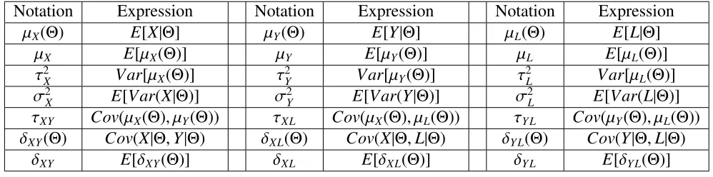
For the convenience of expression, we give a table of our notations in the thesis. That is,
Notation Expression Notation Expression Notation Expression µX(Θ) E[X|Θ] µY(Θ) E[Y|Θ] µL(Θ) E[L|Θ]
µX E[µX(Θ)] µY E[µY(Θ)] µL E[µL(Θ)]
τ2
X Var[µX(Θ)] τ
2
Y Var[µY(Θ)] τ
2
L Var[µL(Θ)]
σ2
X E[Var(X|Θ)] σ
2
Y E[Var(Y|Θ)] σ
2
L E[Var(L|Θ)]
τXY Cov(µX(Θ), µY(Θ)) τXL Cov(µX(Θ), µL(Θ)) τY L Cov(µY(Θ), µL(Θ))
δXY(Θ) Cov(X|Θ,Y|Θ) δXL(Θ) Cov(X|Θ,L|Θ) δY L(Θ) Cov(Y|Θ,L|Θ)
δXY E[δXY(Θ)] δXL E[δXL(Θ)] δY L E[δY L(Θ)]
Table 2.1: A list of notations
Using the notation above, the left-hand side of Equation (2.12) can be rewritten as
Cov(Xn+1,Yi) = E[Xn+1Yi]−E[Xn+1]E[Yi]
= E
E[Xn+1Yi|Θ] −E[µX(Θ)]E[µY(Θ)]
= E
E[Xn+1|Θ]E[Yi|Θ] −E[µX(Θ)]E[µY(Θ)]
= E[µX(Θ)µY(Θ)]−E[µX(Θ)]E[µY(Θ)]
= Cov(µX(Θ), µY(Θ))
= τXY,
fori = 1, . . . ,nand the reason of the third step is independence of Xi andXn+1conditional on Θ.
Under the same reason, we have
Cov(Yj,Yi)=τ2Y and Cov(Lj,Yi)= τY L,
2.1. General results 15
Now, we rewrite Equation (2.12) as
τXY = n
X
j=1
j,i ˆ
αY jCov(Yj,Yi)+αˆYiVar(Yi)+ n
X
j=1
j,i ˆ
αL jCov(Lj,Yi)+αˆLiCov(Li,Yi) (2.14)
=
n
X
j=1
j,i ˆ
αY jτ2Y+αˆYi(σ2Y+τ
2
Y)+ n
X
j=1
j,i ˆ
αL jτY L+αˆLi(δY L+τY L) (2.15)
=
n
X
j=1
ˆ
αY jτ2Y+αˆYiσ2Y+ n
X
j=1
ˆ
αL jτY L+αˆLiδY L, (2.16)
where
Var(Yi) = E[Var(Yi|Θ)]+Var[E(Yi|Θ)] (2.17)
= σ2
Y+Var[µY(Θ)] (2.18)
= σ2
Y+τ
2
Y, (2.19)
Cov(Li,Yi) = E[Cov(Li|Θ,Yi|Θ)]+Cov(E[Li|Θ],E[Yi|Θ]) (2.20)
= E[Cov(L|Θ,Y|Θ)]+Cov(µL(Θ), µY(Θ)) (2.21)
= δY L+τY L. (2.22)
Compared with (2.16), Equation (2.13) can be rewritten as
τXL= n
X
j=1
ˆ
αY jτY L+αˆYiδY L+ n
X
j=1
ˆ
αL jτ2L+αˆLiσ2L, (2.23)
fori= 1, . . . ,n.
Next, mutiply (2.16) byσ2Land mutiply (2.23) byδY L, then subtract each other to obtain
ˆ αYi =
τXYσ2L−τXLδY L−(τ2Yσ2L−τY LδY L)P n
j=1αˆY j−(τY Lσ2L−τ2LδY L)P n
j=1αˆL j
σ2
Yσ
2
L−δ
2
Y L
, (2.24)
ifσ2
Yσ
2
L ,δ
2
Y Land fori=1, . . . ,n.
We notice that the right-hand side of Equation (2.24) does not depend oni. So we have that ˆ
αY j= αˆYifori, jandi, j= 1, . . . ,n. We let them be ˆαY. With the same reason, we let all ˆαLi
be ˆαLfori=1, . . . ,n. Then, we have
τXY = αˆY(nτ2Y +σ
2
Y)+αˆL(nτY L+δY L),
τXL = αˆY(nτY L+δY L)+αˆL(nτ2L+σ
2
L),
which can be rewritten in matrix form as
nτ2Y +σ2Y nτY L+δY L
nτY L+δY L nτ2L+σ2L
!
ˆ αY
ˆ αL
!
= τXY
τXL
!
16 Chapter2. Two-dimensional semi-linear credibility model
Hence, ˆαY and ˆαLhave a unique solution,
ˆ αY =
τXY(nτ2L+σ
2
L)−τXL(nτY L+δY L)
(nτ2Y +σ2Y)(nτ2L+σ2L)−(nτY L+δY L)2
, (2.26)
ˆ αL =
τXL(nτ2Y+σ2Y)−τXY(nτY L+δY L)
(nτ2
Y +σ
2
Y)(nτ
2
L+σ
2
L)−(nτY L+δY L)2
, (2.27)
if
(nτ2Y+σ
2
Y)(nτ
2
L+σ
2
L), (nτY L+δY L)2. (2.28)
LetArepresent (nτ2
Y+σ
2
Y),Brepresentnτ
2
L+σ
2
LandCrepresent (nτY L+δY L). The matrix
becomes
nτ2
Y +σ
2
Y nτY L+δY L
nτY L+δY L nτ2L+σ
2
L
!
= A C
C B
!
.
If the determinant of this matix is zero, that is AB = C2. Then, there are no solution for
Equation (2.25) ifτXY/τXL,C/B, and there are infinite solutions ifτXY/τXL =C/B. For details
of matrix with zero determinant, readers are referred to Marcus et al. [9].
Now, we get the value of ˆαY and ˆαL. Then, we can get the value of ˆα0from Equation (2.11).
That is
ˆ
α0= µX−nαˆYµY−nαˆLµL. (2.29)
Now, we get the new credibility premium from (2.1). That is
d
µX(θ) = αˆ0+αˆY n
X
j=1
Yj+αˆL n
X
j=1
Lj (2.30)
= µX−nαˆYµY−nαˆLµL+nαˆYY¯ +nαˆLL¯ (2.31)
= µX+nαˆY( ¯Y −µY)+nαˆL( ¯L−µL), (2.32)
2.1. General results 17
2.1.2
The minimum value of MSE
Next, we also need to calculate the minimum value of MSE (2.2) because we will compare it with the MMSEs of non-split credibility and semi-linear credibility. So, we have
ˆ
Q = E
(
µn+1(Θ)−µdX(Θ)
2)
(2.33)
= E
(
µn+1(Θ)−αˆ0−nαˆYY¯ −nαˆLL¯
2)
(2.34)
= E
"
µn+1(Θ)−nαˆYY¯
2
+αˆ0+nαˆLL¯
2
−2
µn+1(Θ)−nαˆYY¯
ˆ
α0+nαˆLL¯
#
(2.35)
= Eµn+1(Θ)2
+n2αˆY2E
¯
Y2−2nαˆYE
µn+1(Θ) ¯Y
+αˆ02+n2αˆL2E
¯
L2+2nαˆ0αˆLE
¯ L
−2 ˆα0E(µn+1(Θ))−2nαˆLE
µn+1(Θ) ¯L
+2nαˆ0αˆYE
¯
Y+2n2αˆLαˆYE
¯
YL¯ (2.36)
= τ2
X+µ
2
X +n
2
ˆ αY2
1 nσ
2
Y +τ
2
Y+µ
2
Y
!
−2nαˆY(τXY +µXµY)+αˆ02
+n2αˆL2
1 nσ
2
L+τ2L+µ2L
!
+2nαˆ0αˆLµL−2 ˆα0µX −2nαˆL(τXL+µXµL)
+2nαˆ0αˆYµY+2n2αˆLαˆY
1
nδY L+τY L+µYµL
!
(2.37)
= τ2
X−µ
2
X +nαˆY2σ2Y+n
2
ˆ
αY2τ2Y−n
2
ˆ
αY2µ2Y +(µX −nαˆYµY −nαˆLµL)2
+nαˆL2σ2L+n2αˆL2τ2L−n2αˆL2µ2L+2n(µX −nαˆYµY) ˆαLµL+2nαˆYµXµY
+2nαˆLαˆYδY L+2n2αˆLαˆYτY L−2nαˆYτXY −2nαˆLτXL (2.38)
= τ2
X+nαˆY2σ2Y +n
2αˆ
Y2τ2Y−2nαˆYτXY
+nαˆL2σ2L+n
2αˆ
L2τ2L−2nαˆLτXL
+2nαˆLαˆYδY L+2n2αˆLαˆYτY L, (2.39)
where ˆαLand ˆαY meet Equation (2.25).The details of why Equation (2.36) goes to (2.37) will
be seen in Appendix A.
Remark The minimum value of MSE above(or called ˆQ) is the minimum value given by one
K in our model. Giving a differentK will result in a different MMSE.
2.1.3
Summary
In summary, we give two Theorems as follows.
Theorem 2.1.1 The two-dimensional semi-linear credibility estimator ofµX(θ) in the simple
B¨uhlmann model, based on two different transformed data Yj = f(Xj)and Lj = g(Xj), is given
by
d
µX(θ)=µX +nαˆY( ¯Y−µY)+nαˆL( ¯L−µL),
where( ˆαY,αˆL)satisfies
nτ2Y +σ2Y nτY L+δY L
nτY L+δY L nτ2L+σ2L
!
ˆ αY
ˆ αL
!
= τXY
τXL
!
18 Chapter2. Two-dimensional semi-linear credibility model
or
ˆ αY =
τXY(nτ2L+σ2L)−τXL(nτY L+δY L)
(nτ2
Y +σ
2
Y)(nτ
2
L+σ
2
L)−(nτY L+δY L)2
,
ˆ αL =
τXL(nτ2Y+σ2Y)−τXY(nτY L+δY L)
(nτ2Y +σ2Y)(nτ2L+σ2L)−(nτY L+δY L)2
,
if(nτ2Y+σ2Y)(nτ2L+σ2L), (nτY L+δY L)2.
Theorem 2.1.2 The minimum mean square error of the two-dimensional semi-linear
credibil-ity estimator in the simple B¨uhlmann model is given by
ˆ Qmin= E
(
µn+1(Θ)−α0−
n
X
j=1
αY jYj− n
X
j=1
αL jLj
2)
= τ2
X +nαˆY2σ2Y+n
2αˆ
Y2τ2Y −2nαˆYτXY
+nαˆL2σ2L+n
2
ˆ
αL2τ2L−2nαˆLτXL
+2nαˆLαˆYδY L+2n2αˆLαˆYτY L.
Remarks The two-dimensional semi-linear credibility model includes non-split credibility
model and semi-linear credibility model. It will be semi-linear credibility model if Yj =
f(Xj) = g(Xj) = Lj for j = 1, . . . ,n. Furthermore, it will be non-split credibility model if
Yj = f(Xj)= Xj = g(Xj)= Lj for j=1, . . . ,n.
In general, condition (2.28) will not be met if Yj = f(Xj) = g(Xj) = Lj for j = 1, . . . ,n,
which means that we will not be able to use Equations (2.26) and (2.27) to get the optimalα’s. However, Equation (2.25) will always be established whatever the transformed data are.
2.2
Split results
According to Section 1.3, split credibility model has two different partial losses, primary loss and excess loss. So, generally, we should let Yj be the primary loss and let Lj be the excess
2.2. Split results 19
parameters is as follows,
µX(θ) = α0+αp n
X
j=1
Xp j+αe n
X
j=1
Xe j
= α0+αp n
X
j=1
Xp j+αe n
X
j=1
(Xj−Xp j)
= α0+(αp−αe) n
X
j=1
Xp j+αe n
X
j=1
Xj
= α0+αY n
X
j=1
Yj+αL n
X
j=1
Lj
= α0+αY n
X
j=1
Yj+αX n
X
j=1
Xj,
whereXp j = min(Xj,K) andXe j = Xj−Xp j as well asK is a split point. In the meantime, we
change the notationαLtoαX and change the notationLtoX.
Hence, we should have
ˆ
αp = αˆY +αˆL= αˆY +αˆX, (2.40)
ˆ
αe = αˆL=αˆX. (2.41)
In this way, we have the accurate expressions of credibility premium and MMSE as follows,
d
µX(θ) = µX +nαˆY( ¯Y−µY)+nαˆX( ¯X−µX) (2.42)
= µX +ZbY( ¯Y −µY)+cZX( ¯X−µX), (2.43)
where ˆαY and ˆαX meet
nτ2Y+σ2Y nτXY +δXY
nτXY +δXY nτ2X+σ2X
!
ˆ αY
ˆ αX
!
= τXY
τ2
X
!
, (2.44)
and
ˆ
Q = τ2X +nαˆY2σ2Y+n
2αˆ
Y2τ2Y−2nαˆYτXY
+nαˆX2σ2X+n
2αˆ
X2τ2X −2nαˆXτ2X
+2nαˆXαˆYδXY +2n2αˆXαˆYτXY (2.45)
= τ2
X +
1
nZbY
2
σ2
Y +ZbY
2
τ2
Y −2ZbYτXY
+1
ncZX
2
σ2
X+cZX
2
τ2
X −2cZXτ2X
+2
20 Chapter2. Two-dimensional semi-linear credibility model
Again, we letArepresent (nτ2Y +σ2Y), Brepresentnτ2X +σ2X andCrepresent (nτXY +δXY).
The matrix becomes
nτ2Y+σ2Y nτXY +δXY
nτXY +δXY nτ2X+σ2X
!
= CA CB !
. (2.47)
If the determinant of this matix is zero, there are no solution for Equation (2.44) ifτXY/τ2X ,
C/B, and there are infinite solutions ifτXY/τ2X =C/B. For details of matrix with zero
determi-nant, readers are referred to Marcus et al. [9].
In general, A andBare not equal to 0, but A = 0 when K = 0. In this situation,τXY = 0,
C= 0,Y =0 and our credibility model becomes non-split credibility model.
When we have infinite solutions, the solution of non-split credibility model is also a solution for us in our credibility model, which means that the minimum value of MSE in our credibility model is same as the minimum value of MSE in non-split credibility model. Hence, we choose the solution of non-split credibility model as the solution of our credibility model in this time.
2.2.1
Properties of credibility
Before we study the optimal split point, we present some properties of credibility. This will help us gain intuition and make practical sense of our model.
Rewrite Equation (2.25) as
c
ZX =
nτXY
nτXY +δXY
− nτ
2
Y+σ
2
Y
nτXY +δXY
b
ZY, (2.48)
b
ZY =
nτ2X nτXY +δXY
− nτ
2
X+σ
2
X
nτXY +δXY
c
ZX, (2.49)
if nτXY +δXY , 0. In general, this condition should be always met because if X < K, then
Y = XandτXY would beτ2X, which is always bigger than zero exceptµX(Θ) is a constant but it
should not be happened, as well asδXY would beσ2X, whose property is same asτ2X. Otherwise,
Y would be always equal toK and we would getnτXY +δXY = 0. In an extreme case which is
that all ofXare bigger or equal toK, our model would become non-split credibility model and this situation would be the same asK =0.
Letn→+∞, (2.48) and (2.49) become
c
ZX = 1−
τ2
Y
τXY
b
ZY, (2.50)
b
ZY =
τ2
X
τXY
− τ
2
X
τXY
c
ZX, (2.51)
thus we getcZX → 1 andZbY → 0 ifτ2XY ,τ
2
Xτ
2
Y. In general, this condition is met exceptY = X
orK = 0 orK → +∞. As we all know, we should give more credibility to the data if there are a lot of losses we get. The properties of credibility above meet our expectation.
For the time being, we don’t restrictY =min(X,K) and let it can be any functions onXfor now and go to find the influences of parametersτXY andδXY.
LetτXY → ∞, we getcZX → 1 andZbY → 0. From the results, we know that this influence
2.2. Split results 21
them will cause more credibility on X. Notice that the value can be either very small or very large.
Similarly, let δXY → ∞, we get cZX → 0 and ZbY → 0. From the results, we know that
we should use the manual rate, µX, to estimate the future loss if we choose a function on X,
Y = f(X), with a large value of δXY. Notice that the value can be either very small or very
large.
Remarks In the above, we discuss the sensitivity of the credibility to the values of a parameter assuming that other parameters remain unchanged. In fact, other paramters may be changed withτXY orδXY, but we don’t consider this situation here. So, further research can be whether
any other parameters would be changed or not when the parameters we specify change if you are interested in these results and want to explore more.
Notice that the credibility of primary loss, Zbp, is equal to ZbY +cZX and the credibility of
excess loss,Zbe, is equal tocZX. We are not able to ensure that Zbp andZbe are between 0 and 1 as
commented in Robbin [11].
2.2.2
The optimal split point
The optimal split point minimizes the mean square error. Let the MMSE of non-split credibility be ˆQnsp, the MMSE of semi-linear credibility be ˆQtsland the MMSE of two-dimensional
semi-linear credibility be ˆQtdsl. From (1.17), (1.47) and (2.45), we respectively have
ˆ Qnsp =
σ2
Xτ
2
X
σ2
X +nτ
2
X
, (2.52)
ˆ
Qtsl = τ2X−
nτ2XY σ2
Y+nτ
2
Y
, (2.53)
ˆ
Qtdsl = τ2X+nαˆY2σ2Y+n2αˆY2τ2Y −2nαˆYτXY
+nαˆX2σ2X +n
2αˆ
X2τ2X−2nαˆXτ2X
+2nαˆXαˆYδXY +2n2αˆXαˆYτXY. (2.54)
We notice that ˆQtdsl is a function of the split point,K, because ˆαX, ˆαY,µY, σ2Y,τ
2
Y, δXY and
τXY are functions on K. In theory, we take derivatives of ˆQtdsl with respect to K and let the
expression equal to zero for getting the optimal split point, ˆK. In the mathematical formula, it is
∂Qˆtdsl ∂Kˆ =0.
22 Chapter2. Two-dimensional semi-linear credibility model
Lemma 2.2.1 (Leibniz’s Rule) Let A⊂ Rnbe open, let I =[a,b]⊂ Rbe a compact interval, and let f be a (jointly) continuous mapping of A×I into R. Letαandβbe two continuously differentiable mappings of A into I. Then
g(x)=
Z β(x)
α(x)
f(x,t)dt,
is continuous in A. If in addition, the partial derivative ∂∂fx exists and is (jointly) continuous on A×I, then g is continuously differentiable on A and
g0(x)=
Z β(x) α(x)
∂f(x,t)
∂x dt+ f(x, β(x))β 0
(x)− f(x, α(x))α0(x).
Notice that the conditional mean of Y = Xp is the function onX andK. Under the integral
expression, the integral interval is only related to K and the function is only integrated on X. Therefore, we can use the Leibniz’s Rule to get our partial differential equations. Suppose that the losses, X, have the same distribution with pdf, fX|Θ(x), and cdf,FX|Θ(x), conditional on Θ. LetY =min(X,K), then
µY(Θ)=
Z K
0
x fX|Θ(x)dx+K(1−FX|Θ(K)).
Under the Leibniz’s Rule, we take partial derivative ofµY(Θ) with respect toK, then
∂µY(Θ)
∂K =
Z K
0
∂ x fX|Θ(x)
∂K dx+K fX|Θ(K)−0fX|Θ(0)
+1−FX|Θ(K)−K fX|Θ(K)
= K fX|Θ(K)+1−FX|Θ(K)−K fX|Θ(K)
= 1−FX|Θ(K).
Using the same method, all of the partial differential equations of parameters are derived. In the end, the numerical solution ofKshould be obtained. However, we guess that the solution would be so complex that it is not easy to be used in reality and we give another way to get it. Let us turn to research for size relationships between ˆQnsp, ˆQtsl and ˆQtdsl. Then, we get a
Theorem as follows,
Theorem 2.2.2 Let the MMSE of non-split credibility beQˆnsp, the MMSE of semi-linear
cred-ibility be Qˆtsl and the MMSE of two-dimensional semi-linear credibility be Qˆtdsl. Then, Qˆtdsl
will be the minimum value between them, that is,
ˆ
Qtdsl ≤ Qˆnsp and Qˆtdsl ≤ Qˆtsl,
whereQˆnspis (2.52), Qˆtslis (2.53) andQˆtdsl is (2.54).
Proof: We only proof the first inequality, ˆQtdsl ≤ Qˆnsp, and the other’s proof is similar. Notice
that when ˆαY is equal to 0, we have
ˆ
Qtdsl = τ2X +nαˆX2σ2X+n
2
ˆ
αX2τ2X−2nαˆXτ2X
2.2. Split results 23
where ˆαX =
τ2
X σ2
X+nτ
2
X
. Then,
ˆ
Qtdsl = nαˆX2σ2X +(1−nαˆX)2τ2X
= nτ 4
Xσ
2
X
(σ2
X+nτ
2
X)2
+ σ
4
Xτ
2
X
(σ2
X +nτ
2
X)2
= σ
2
Xτ
2
X
σ2
X+nτ
2
X
= Qˆnsp,
which shows again that the two-dimensional semi-linear credibility includes non-split credibil-ity.
Assume that the MMSE of two-dimensional semi-linear credibility, ˆQtdsl, is bigger than
ˆ
Qnsp with the optimal ˆαX and ˆαY where ˆαY , 0. However, we know that we could find the
value of MMSE, ˆˆQtdsl = Qˆnsp as long as we selected ˆˆαY = 0 and ˆˆαX =
τ2
X σ2
X+nτ
2
X
. And we could
get a smaller value. Therefore, ˆQtdsl with the optimal ˆαY , 0 is not the MMSE and it is not
existed.
In total, we have ˆQtdsl ≤ Qˆnspfor all times.
As we said before, if the determinant of matix (2.47) is zero, then there are no solution for Equation (2.44) or the solution of non-split credibility model would be chosen as the solution of our credibility model. However, there is a special case that we do not need to split the losses if the determinant of matrix (2.47) is not zero. We give a Theorem as follows.
Theorem 2.2.3 Assume thatτ2X ,0,τXY ,0andδXY/τXY =σ2X/τ2X, as well as,
nτ2Y +σ2Y nτXY +δXY
nτXY +δXY nτ2X +σ2X
, 0.
Then, the two-dimensional semi-linear credibility model becomes non-split credibility model whatever the split point is.
Proof: Because the determinant of matrix (2.47) is not equal to zero, ˆαY and ˆαX have a unique
solution. And if δXY/τXY = σ2X/τ
2
X, then we know that ( ˆαY,αˆX) = (0, τ2X/(nτ
2
X + σ
2
X)) is a
solution of Equation (2.44) because
ˆ αX =
τXY
nτXY +δXY
= 1
n+ δXY τXY
= 1
n+ σ
2
X τ2
X
= τ
2
X
nτ2
X +σ
2
X
.
Hence, we know that the solution ( ˆαY,αˆX) = (0, τ2X/(nτ
2
X +σ
2
X)) is the unique solution of
24 Chapter2. Two-dimensional semi-linear credibility model
Under Theorem 2.2.3, the split way is invalid and we do not need to split the losses if the conditions of Theorem 2.2.3 are met.
Now we give our method to get the optimal split point. Firstly, we sort the losses,X, from small to large. And then, we take some percentiles as our split point according to the accuracy we need. The more precise, the more points. From our practical experience, the K value generally is chosen a relatively large value, so we can take more points at larger percentiles to determine the best K value.
For example, we could choose the 0th, 25th, 50th, 75th, 80th, 85th, 90th, 95th and 100th percentiles as our split points. Then, we use our formulas to calculate the parameters and the optimalα’s. Next, we calculate the values of MMSE given by different split points. We choose the minimum one and choose the corresponding K value, which is the percentile and would be different in number’s value according to different data, as the future optimal percentile in future data from the same source(or the same group).
In this method, we can not guarantee that the K value we choose is the exact optimal K value for each group of data, but the worst result is only the minimum of MMSE of non-split credibility and MMSE of semi-linear credibility.
2.2.3
Nonparametric estimation
In this section, we consider unbiased estimation of our parameters, µX, τ2X, σ2X, τXY and δXY.
Let us use the simple B¨uhlmann model as an example.
Suppose thatnj = n > 1 for all jand we have policyholders with number ofm > 1. That
is, for policyholderi, we have the loss vector
Xi = (Xi1,Xi2,· · · ,Xin)T, i=1,2,· · · ,m.
Furthermore, conditional onΘi =θi,Xi j has mean
µX(θi)= E(Xi j|Θi = θi),
and variane
VX(θi)=Var(Xi j|Θi = θi),
as well asXisandXitare independent if s, tconditional onΘi =θi. In the meantime,Xi j and
Xstare also independent ifi, sbecause of the independence of different policyholders. So we
have
¯ Xi =
1
n
n
X
j=1
Xi j,
¯
X = 1
nm
m
X
i=1
n
X
j=1
Xi j.
An unbiased estimator ofµX is
2.2. Split results 25
because
E( ˆµX)= E( ¯X) =
1
nm
m
X
i=1
n
X
j=1
E(Xi j)
= 1
nm
m
X
i=1
n
X
j=1
E(µX(Θi))
= 1
nm
m
X
i=1 n
X
j=1
µX
= µX.
At the same time, an unbiased estimator of the conditional variance ofXi jis
d
VX(Θi)=
1
n−1
n
X
j=1
(Xi j−X¯i)2.
Hence, an unbiased estimator ofσ2
X is
c
σ2
X = E(VXd(Θi)) =
1
m
m
X
i=1 d
VX(Θi)
= 1
m(n−1)
m
X
i=1
n
X
j=1
(Xi j−X¯i)2.
For details, readers are referred to Klugman et al. [8]. We now turn to determine unbiased estimator ofτ2
X. Since
Var( ¯Xi) = Var
h
E( ¯Xi|Θi)
i
+EhVar( ¯Xi|Θi)
i
= Varµ
X(Θi)+E
VX(Θi)
n
= τ2
X+
σ2
X
n , an unbiased estimator ofτ2X is
b
τ2
X = Vard( ¯Xi)−
c
σ2
X
n
= 1
m−1
m
X
i=1
( ¯Xi−X¯)2−
c
σ2
X
n
= 1
m−1
m
X
i=1
( ¯Xi−X¯)2−
1
mn(n−1)
m
X
i=1 n
X
j=1
26 Chapter2. Two-dimensional semi-linear credibility model
whereσc2
X is given and
d
Var( ¯Xi)=
1
m−1
m
X
i=1
( ¯Xi −X¯)2.
ForµY,τ2Y andσ2Y, we firstly get the dataY from the losses X. In our case,Y = min(X,K)
given a split pointK. Then, their unbiased estimators are
ˆ
µY = Y¯ =
1
nm
m
X
i=1
n
X
j=1
Yi j,
c
σ2
Y = E(VYd(Θi))=
1
m(n−1)
m
X
i=1
n
X
j=1
(Yi j−Y¯i)2,
b
τ2
Y = Vard( ¯Yi)−
c
σ2
Y
n
= 1
m−1
m
X
i=1
( ¯Yi−Y¯)2−
1
mn(n−1)
m
X
i=1
n
X
j=1
(Yi j−Y¯i)2.
For estimation ofτXY andδXY, we firstly consider an unbiased estimator of the covariance.
Suppose that S1,S2,· · · ,Sr are independent random variables with same mean µS = E(Sj)
andT1,T2,· · · ,Trare independent random variables with same meanµT = E(Tj). And we are
only talking about paired data whereSiandTj are only correlated wheni= j.
Let
¯
S = 1
r
r
X
j=1
Sj,
¯
T = 1
r
r
X
j=1
Tj.
Then, consider the statisticPr
j=1(Sj−S¯)(Tj−T¯). It can be rewritten as
r
X
j=1
(Sj −S¯)(Tj−T¯) = r
X
j=1
(SjTj−SjT¯ −TjS¯ +S¯T¯)
=
r
X
j=1
SjTj−rS¯T¯ −rS¯T¯ +rS¯T¯)
=
r
X
j=1
2.2. Split results 27
Taking expectation of both sides yields
E r X j=1
(Sj−S¯)(Tj−T¯)
= E r X j=1
SjTj
−rE( ¯ST¯)
= E r X j=1
SjTj
−rhCov( ¯S,T¯)+µSµT
i = E r X
j=1
SjTj
−r
Cov(1 r
r
X
j=1
Sj,
1
r
r
X
j=1
Tj)+µSµT
= E r X
j=1
SjTj
−r 1
r2Cov(
r
X
j=1
Sj, r
X
j=1
Tj)+µSµT
= E r X j=1
SjTj
− 1 r r X j=1
Cov(Sj,Tj)−rµSµT
= E r X
j=1
SjTj
−Cov(S,T)−rµSµT
= rE(S T)−Cov(S,T)−rµSµT
= r
E(S T)−µSµT−Cov(S,T)
= (r−1)Cov(S,T).
Therefore, an unbiased estimator of the covariance is r−11Pr
j=1(Sj−S¯)(Tj−T¯).
To estimateδXY, notice that we have an unbiased estimator ofδXY(Θi) as follows,
d
δXY(Θi)=
1
n−1
n
X
j=1
(Xi j−X¯i)(Yi j−Y¯i).
Hence, an unbiased estimator ofδXY is
ˆ
δXY =E(δXYd(Θi)) =
1
m
m
X
i=1 d
δXY(Θi)
= 1
m(n−1)
m
X
i=1
n
X
j=1
(Xi j−X¯i)(Yi j−Y¯i).
Now we consider the value of Cov( ¯Xi,Y¯i). Recall that Xi1,Xi2,· · · ,Xin are independent
28 Chapter2. Two-dimensional semi-linear credibility model
conditional onΘi =θi. Then
Cov( ¯Xi,Y¯i) = E
h
Cov( ¯Xi|Θi,Y¯i|Θi)
i
+CovhE( ¯Xi|Θi),E( ¯Yi|Θi)
i
= E
Cov(1 n
n
X
j=1
Xi j|Θi,
1
n
n
X
j=1
Yi j|Θi)
+
Cov(µX(Θ), µY(Θ))
= E
1
n2Cov(
n
X
j=1
Xi j|Θi, n
X
j=1
Yi j|Θi)
+
τXY
= E
1
n2
n
X
j=1
Cov(Xi j|Θi,Yi j|Θi)
+
τXY
= E
1
nCov(X|Θ,Y|Θ)
+τXY = δXY
n +τXY.
We also have an unbiased estimator ofCov( ¯Xi,Y¯i) as follows,
d
Cov( ¯Xi,Y¯i)=
1
m−1
m
X
i=1
( ¯Xi−X¯)( ¯Yi−Y¯).
Thus, we get an unbiased estimator ofτXY. That is,
ˆ
τXY = Covd( ¯Xi,Y¯i)−
ˆ δXY
n
= 1
m−1
m
X
i=1
( ¯Xi−X¯)( ¯Yi−Y¯)−
1
mn(n−1)
m
X
i=1
n
X
j=1
(Xi j −X¯i)(Yi j −Y¯i).
Now, we give all unbiased estimation of our needed parameters and you can review the whole results of this section in Appendix B.
2.2.4
The estimators of
µ
p(
θ
)
and
µ
e(
θ
)
Besides the estimator ofµX(θ), we also concern about the estimators of primary part(µp(θ)) and
excess part(µe(θ)). In reality, the large claims generally are large relative to all of data and we
do not want that they occupy so large proportion that it will influence our future income as well as increase risk and instability. In the other words, we hope that the mean of the excess part is very small to reduce the overall impact of that part. Therefore, we could control the influence and risk if we could estimateµp(θ) andµe(θ).
We discuss µe(θ) only and the other is similar. LetY be Xp = min(X,K) and L be Xe =
X −Xp. Thenµp(Θ) = µY(Θ) andµe(Θ) = µL(Θ). And we let the estimator ofµp(θ) beµdp(θ)
2.2. Split results 29
We still useYs and Xs as data to estimateµe(θ). Because the independence ofLis the same as
X, the processes are the same as the processes of the estimator ofµX(θ). Therefore, we have
d
µe(θ)=µdL(θ) = βˆ0+βˆY n
X
j=1
Yj+βˆX n
X
j=1
Xj
= µL−nβˆYµY −nβˆXµX+nβˆYY¯ +nβˆXX¯
= µL+nβˆY( ¯Y−µY)+nβˆX( ¯X−µX),
compared with (2.32) as well as where ˆβX and ˆβY meet
nτ2Y+σ2Y nτXY +δXY
nτXY +δXY nτ2X+σ2X
! βˆ
Y
ˆ βX
!
= τY L
τXL
!
, (2.55)
compared with (2.44). Because we only want to use the parameters we have used and calcu-lated, we rewriteτY LandτXL as
τY L = Cov(µY(Θ), µL(Θ))
= Cov(µY(Θ), µX(Θ)−µY(Θ))
= Cov(µY(Θ), µX(Θ))−Cov(µY(Θ), µY(Θ))
= τXY −Var[µY(Θ)]
= τXY −τ2Y,
τXL = Cov(µX(Θ), µL(Θ))
= Cov(µX(Θ), µX(Θ)−µY(Θ))
= Cov(µX(Θ), µX(Θ))−Cov(µX(Θ), µY(Θ))
= Var[µX(Θ)]−τXY
= τ2
X −τXY,
because
µX(Θ) = E[X|Θ]= E[Xp+Xe|Θ]= E[Y+L|Θ]= E[Y|Θ]+E[LΘ]
= µY(Θ)+µL(Θ)=µp(Θ)+µe(Θ),
µX = µY+µL=µp+µe.
Forµp(θ), we change ˆα0to be ˆγ0, ˆαYto be ˆγYand change ˆαX to be ˆγX. The estimator is
d
µp(θ)= µdY(θ) = γˆ0+γˆY n
X
j=1
Yj+γˆX n
X
j=1
Xj
= µY−nγˆYµY−nγˆXµX +nγˆYY¯ +nγˆXX¯
= µY+nγˆY( ¯Y−µY)+nγˆX( ¯X−µX),
where
nτ2Y+σ2Y nτXY +δXY
nτXY +δXY nτ2X +σ2X
!
ˆ γY
ˆ γX
!
= τ2Y
τXY
!
30 Chapter2. Two-dimensional semi-linear credibility model
Notice that the right-hand side of Equation (2.44) is the sum of the right-hand side of Equation (2.55) and the right-hand side of Equation (2.56). That is,
d
µX(θ)=µdp(θ)+µde(θ),
which meets our expectation. Now, we can estimate µp(θ) andµe(θ). More elegantly, using
matrix notation we can write
d
µX(θ)
d
µp(θ)
d
µe(θ)
=
µX
µY
µL
+
nαˆY nαˆX
nγˆY nγˆX
nβˆY nβˆX
¯ Y −µY
¯ X−µX
!
, (2.57)
Chapter 3
Examples
In this chapter, we discuss three examples. The first one is that the losses follow an Exponential distribution conditional on risk parameters. The second one is that the losses follow a Poisson distribution conditional on risk parameters. The final one is that the losses follow a mixture of two Exponential distributions where one distribution is conditional on risk parameters. All of risk parameters,Θ, follow a Gamma distribution.
3.1
Exponential distribution conditional on
Θ
We consider an example much like the collective risk model (CRM) in Robbin [11]. Suppose that the losses Xi1,Xi2,Xi3, . . . ,Xin conditional on Θi = θi follow an Exponential distribution
with the same mean and same variance as well asΘfollows a Gamma distribution with shape parameter,α, and rate parameter,β. Let fX|Θ(x) be the probability density function(pdf) of the losses conditional onΘand fΘ(θ) be the pdf of theΘ. LetFX|Θ(x) be the cumulative distribution function(cdf) of the losses conditional onΘ. Then, we have
fX|Θ=θ(x) = θe −θx,
(3.1) FX|Θ=θ(x) = 1−e−θx, (3.2)
fΘ(θ) = β α
Γ(α)θα −1
e−βθ. (3.3)
Hence, the mean and variance of losses conditional onΘas well as the mean and variance ofΘare
E(X|Θ =θ)= 1
θ, (3.4)
Var(X|Θ =θ)= 1
θ2, (3.5)
E(Θ)= α
β, (3.6)
Var(Θ)= α
β2. (3.7)
32 Chapter3. Examples
Assume that there are m = 6 policyholders. Each policyholder’s risk parameter is repre-sented by a random variable Θ = (Θ1 = θ1,Θ2 = θ2, . . . ,Θ6 = θ6), which follows a Gamma
distribution with shape parameter, α = 6, and rate parameter,β = 50. For each policyholder, conditional on Θi = θi, n = 45 past losses are observed. Then, we use R code to randomly
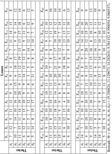
generate risk parameters and losses. For details of data, readers are referred to Table 3.1 and for details of R code, readers are referred to Appendix C.
3.1.1
Parametric estimation
By (3.4),µX(θ)= E(X|Θ =θ)=1/θ. Thus, the unconditional mean ofXis
µX =E[µX(Θ)]=E
1
Θ
=
Z 1
θfΘ(θ)dθ,
= Z 1θ β
α
Γ(α)θα −1
e−βθdθ,
=
Z βα Γ(α)θα
−2
e−βθdθ,
= Z αβ
−1 βα−1 Γ(α−1)θ
α−2e−βθ dθ,
= αβ
−1
Z βα−1 Γ(α−1)θ
α−2e−βθ dθ,
= αβ
−1. (3.8)
The unconditional variance ofX is
σ2
X = E[Var(X|Θ)]= E
1
Θ2
=
Z 1
θ2
βα
Γ(α)θα −1
e−βθdθ,
=
Z βα Γ(α)θα
−3
e−βθdθ,
= β
2
(α−1)(α−2)
Z βα−2 Γ(α−2)θ
α−3
e−βθdθ,
= β
2
(α−1)(α−2), (3.9)
whereΓ(α)=(α−1)Γ(α−1).
Hence, we can calculateτ2X as follows,
τ2
X =Var[µX(Θ)]= Var
1
Θ
= E
1
Θ2
−E
1
Θ 2
,
= β
2
(α−1)(α−2)− β2
(α−1)2,
= β
2