The Stability of Temperate Lakes Under the Changing Climate

(1)

Scholarship@Western

Electronic Thesis and Dissertation Repository

9-27-2019 10:30 AM

The Stability of Temperate Lakes Under the Changing Climate

Aleksey Paltsev

The University of Western Ontario

Supervisor Creed, Irina

The University of Western Ontario Trick, Charles

The University of Western Ontario Graduate Program in Biology

A thesis submitted in partial fulfillment of the requirements for the degree in Doctor of Philosophy

Follow this and additional works at: https://ir.lib.uwo.ca/etd

Part of the Biogeochemistry Commons, Biology Commons, Climate Commons, Environmental Sciences Commons, Fresh Water Studies Commons, Other Ecology and Evolutionary Biology Commons, Other Oceanography and Atmospheric Sciences and Meteorology Commons, and the Terrestrial and Aquatic Ecology Commons

Recommended Citation Recommended Citation

Paltsev, Aleksey, "The Stability of Temperate Lakes Under the Changing Climate" (2019). Electronic Thesis and Dissertation Repository. 6658.

https://ir.lib.uwo.ca/etd/6658

This Dissertation/Thesis is brought to you for free and open access by Scholarship@Western. It has been accepted for inclusion in Electronic Thesis and Dissertation Repository by an authorized administrator of

(2)

ii

Abstract

There is a collective prediction among ecologists that climate change will enhance phytoplankton biomass in temperate lakes. Yet there is noteworthy variation in the structure and regulating functions of lakes to make this statement challengeable and, perhaps, inaccurate. To generate a common understanding on the trophic transition of lakes, I examined the interactive effects of climate change and landscape properties on phytoplankton biomass in 12,644 lakes located in relatively intact forested landscapes. Chlorophyll-a (a) concentration was used as a proxy for phytoplankton biomass. Chl-a concentrChl-ation wChl-as obtChl-ained viChl-a Chl-anChl-alyzing LChl-andsChl-at sChl-atellite imChl-agery dChl-atChl-a over Chl-a 28-yeChl-ar period (1984-2011) and using regression modelling. The most common lake trophic state was oligotrophic (median Chl-a < 2.6 μg L-1), while the least common was

hyper-eutrophic (median Chl-a > 56 μg L-1_{). Lake volume was the most important factor in} determining the present trophic state of the lakes. The majority of the lakes (91.6%) did not show a change in trophic state over an almost 3-decade long sampling period; only 4.0% of the lakes became more eutrophic, and 4.4% of the lakes became more

oligotrophic. Lakes with smaller volumes were further responsive to temperature (warmer lakes were more eutrophic), while lakes with larger volumes were more responsive to precipitation (wetter lakes were more oligotrophic). Early warning

indicators of change in trophic state were examined in the patterns of the residuals of the time series of Chl-a once non-stationary and stationary trends were removed.

(3)

iii

Keywords

(4)

iv

Summary for Lay Audience

(5)

v

Co-Authorship Statement

The PhD thesis contains three manuscripts. In each of these manuscripts, Aleksey Paltsev will be first author, as he conducted pre-processing of Landsat products (Chapter 2) and statistical analysis; he contributed to design of the research, interpretation of the research results and writing of the manuscripts. In each of these manuscripts, Dr. Irena Creed will be second author, as she contributed to the definition of the research problem,

interpretation of results, synthesis of ideas and editing of the manuscripts.

The PhD thesis is extension of Aleksey Paltsev’s Master of Science research:

“Exploration of spatial and temporal changes in trophic status of lakes in the Northern Temperate Forest Biome using remote sensing” published as a Master’s thesis in 2015. Although in this PhD thesis, Aleksey Paltsev adopted research approach and some ideas initially developed in his Master’s research, all pre-processing steps of Landsat products and statistical analyses (including the development of the regression model) were substantially modified, which resulted in a different set of modelled data. Furthermore, more in-depth analyses were performed, for example the space-time kriging and the Mann-Kendall test. The Master’s thesis is cited throughout the PhD thesis where it is appropriate.

(6)

vi

Acknowledgments

I cannot express the level of gratitude and appreciation I have for my amazing supervisor, Dr. Irena Creed. The past years have been some of the most challenging and inspirational years of my life. Your passion for knowledge and advancing science is second to none, and I am grateful for your dedication to my personal development. We have done amazing and rewarding work together and through this, I have learned a lot. You have helped me advance my passion for knowledge and nature and have always pushed me to do more.

I am grateful to my co-supervisor, Dr. Charles Trick. Your wisdom and extremely valuable comments during my presentations and talks continually kept me afloat.

I would like to thank my PhD advisory committee, Dr. Adam Yates and Dr. Ben Rubin. I am grateful for our time together and your continued dedication to the development and completion of my degree. Your insight and guidance throughout the years has enabled me to be successful.

(7)

vii

List of Tables

Table 2.1 Description of water chemistry and morphometry of Ontario lakes selected for the regression model. (Note: observations identified as outliers are not shown in this table). ... 29

Table 2.2 Description of water chemistry and morphometry of Alberta lakes selected for the regression model. (Note: observations identified as outliers are not shown in this table). ... 30

Table 2.3 Pearson correlation coefficients (r) between optically-related variables (Chl-aobs and DOC) and Landsat TM/ETM+ bands and commonly used band combinations/band algorithms (* p < 0.05; ** p < 0.0001). ln indicates natural log transformed values. ... 35

Table 3.1 Number and proportion of lakes according to the trophic state for all lakes (n = 12,644) and a subset of lakes (n = 275) used for climate and landscape control analysis.61

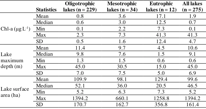
Table 3.2 General descriptive statistics of Chl-amod, maximum depth and surface area of lakes used in this study (n = 275) and for each trophic state. ... 61

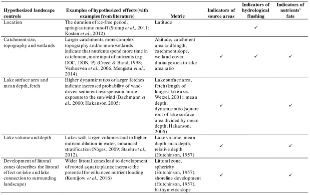
Table 3.3 Hypothesized landscape controls, their possible effects on lakes and proposed metrics to describe the controls... 65

Table 3.4 Pearson correlation coefficients (r) between various landscape (catchment and lake) variables. All variables except latitude, altitude, wetland cover, relative depth, development shoreline, sphericity, and dynamic ratio were ln-transformed. Coefficients in bold indicate significant (p < 0.05) correlation... 68

Table 4.1 Correlation between identified stationary signals and climatic indices. Values in bold show significant correlation at p < 0.1. ... 100

Table A.1 Description of lake samples (sample date, lake morphometry and chemistry) ... 123

(12)

xii

Table A.3 TOA radiance values for Landsat bands 1–5, standard deviation (SD) of radiance in band 5 and TOA reflectance values (with partial atmospheric correction) for Landsat bands 1–4 for 53 ground-sampled lakes. LT = Landsat 5; LE = Landsat 7. ... 129

Table B.1 Parameters of the fitted sum-metric variogram model for ln Chl-amod used in kriging. ... 137

Table C.1 Samples used to evaluate effect of lake DOC on modeled lake Chl-a. ... 141

Table D.1 Samples used to evaluate correlation between lake TP and lake Chl-a. ... 147

(13)

xiii

List of Figures

Figure 1.1 Reflectance spectra of water, Chl-a and CDOM. Colors symbolize Landsat TM/ETM+ bands: blue–B1, green–B2, red–B3, and gray–B4 (near-infrared) (modified from Olmanson et al., 2016). ... 6

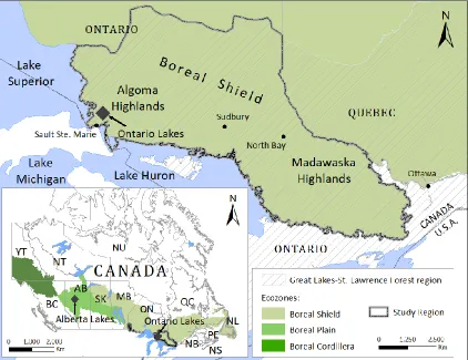
Figure 2.1 Study region (the temperate forest biome) and locations of sampled Ontario and Alberta lakes... 20

Figure 2.2 Schematic model of variation in ln Chl-amod of lakes (modified from Sass et al., 2007). In bold: sources of natural variation in ln Chl-amod (in %) estimated by the two-way ANOVA in this study... 32

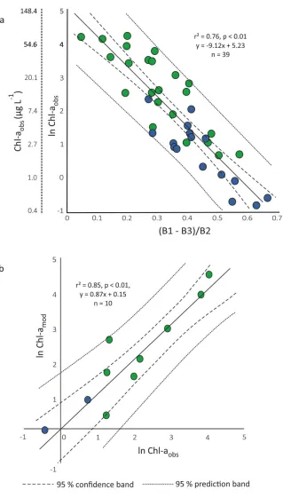
Figure 2.3 (a) Scatterplot of reflectance from (B1-B3)/B2 band algorithm regressed against ln Chl-aobs; (b) comparison of ln Chl-aobs (validation dataset) and ln Chl-amod. The solid line represents the 1:1 line. ... 36

Figure 2.4 Scatterplot of reflectance from (B1-B3)/B2 band algorithm regressed against ln DOC. ... 37

Figure 2.5 (a) Spatial distribution of lakes (based on lake trophic state calculated as median Chl-amod over the 1984–2011 period), and Kernel density of: (b) oligotrophic, (c) mesotrophic, and (d) eutrophic and hypereutrophic lakes. In Kernel density, the default search radius was based on the number of lakes. ... 39

(14)

xiv

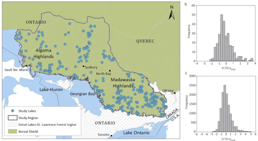
Figure 3.1 (a) Map showing location of the study region (temperate forest biome) and 275 lakes selected for the analysis; and distribution of Chl-a (ln-transformed modelled Chl-a: ln Chl-amod) in (b) 275 lakes (subset of lakes selected for a landscape analysis), and (c) all 12,644 lakes. ... 60

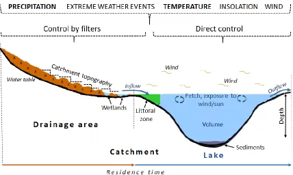
Figure 3.2 Conceptual model of hypothesized climatic (direct and indirect) and landscape controls on Chl-amod of temperate lakes (modified from Hollert et al., 2018). Climatic controls analyzed in the current study are in bold. ... 64

Figure 3.3 (a) Regression tree, and (b) results of the random forests analysis depicting climate and landscape determinants of ln Chl-amod. Panels with colors below the regression tree depict general patterns (increase or decrease) of the most important determinants of ln Chl-amod over an increase ln Chl-amod from left to right. Abbreviations: Pr–precipitation, Tmax–maximum air temperature, V–lake volume, DR–dynamic ratio, WET%–wetland cover, LZ–littoral zone, LAT–latitude; ln indicates ln-transformed values. ... 70

Figure 3.4 Conceptual panels depicting “typical landscape features” for each lake trophic state. Values of climate and landscape determinants of ln Chl-amod are median (except for max depth, for which values are mean). Abbreviations are metrics developed to describe the landscape determinants: V–volume, DR–dynamic ratio. ... 71

Figure 4.1 “Multiple stable states” concept depicted using “stability landscapes” (as exemplified by freshwater lakes). Valleys represent stability domains, in which a stable system, represented by the ball, is kept by internal feedback mechanisms until an external pressure is long and “stressful” enough to move the ball into a new stability domain, where the system reorganizes into a new stable state (modifed from Scheffer et al., 2001). ... 89

Figure 4.2 Map showing location of the study region (the temperate forest biome) and eutrophying (n = 36) and oligotrophying (n = 42) lakes used for the analysis of

(15)

xv

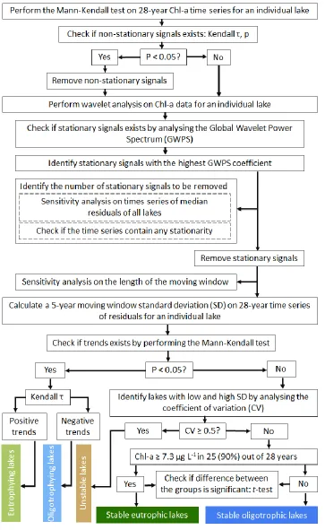
Figure 4.3 Flowchart summarizing steps for removing non-stationary and stationary signals from ln Chl-amod time series and identification lake trophic stability classes. ... 94

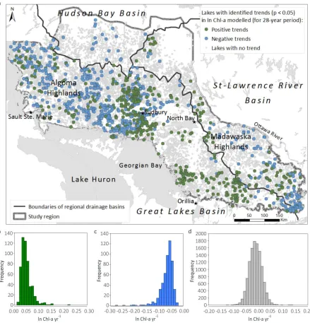
Figure 4.4 Rates of change (slopes) of Chl-amod (ln Chl-a yr-1), max air temperature (Tmax yr-1), precipitation (Pr yr-1) for (a) positive trending lakes (n = 500) and (b) negative trending lakes (n = 561); and (c) Pearson correlation coefficients (r) between ln Chl-a yr-1 for positive and negative trending lakes andclimate forces (i.e., rates of change in max air temperature–Tmax yr-1 and precipitation–P yr-1). Whiskers depict standard deviation. .... 98 Figure 4.5 Sensitivity analysis to identify a threshold when removal of stationary signals should be stopped. Vertical dashed line indicates the threshold (the sixth stationary signal). ... 99

Figure 4.6 (a) Original (de-trended) ln Chl-amod time series (median over 12,644 lakes), and (b–g) stationary signals identified in the time series. Six stationary signals are depicted for all 12,644 lakes (median ln Chl-amod residuals) in accordance with letter from b (first signal) to g (sixth signal). ... 100

Figure 4.7 Temporal distribution of lake stability classes (based on time series of SD5 of residuals from ln Chl-amod) in relation to trophic states (based on ln Chl-amod

concentration). ... 102

Figure 4.8 Spatial distribution and Kernel density of lakes for various lake stability classes (based on time series of SD5 of residuals from ln Chl-amod): (a) stable oligotrophic (n = 5,344), (b) eutrophying (n = 2,605), (c) unstable (n = 1,586), (d) stable eutrophic (n = 146), and (e) oligotrophying (n = 2,963) classes. In Kernel density, the default search radius was based on the number of lakes. ... 103

(16)

xvi

Figure A.1 Location of Ontario lakes within study region, and surficial geology of the study region. ... 132

Figure A.2 Location of Alberta lakes, and surficial geology of the site (Utikuma

Highlands). ... 133

Figure B.1 Number of years (out of entire period: 28 years) of ln Chl-amod data by lake. ... 136

Figure B.2 (a) Sample space–time variogram of residuals from ln Chl-amod; (b) Fitted sum-metric model used in kriging. ... 137

Figure B.3 Prediction accuracy of kriging preformed on ln Chl-amod from 200 randomly selected lakes to interpolate missing values. The solid line represents the 1:1 line. The root means square error (RMSE) of Chl-a interpolation was 0.16. ... 138

Figure C.1 Study region (green area) and location of in-situ Chl-a, TP and DOC data. 144

Figure C.2 Relationship between observed Chl-a and DOC. ... 144

Figure C.3 Relationship between modeled Chl-a and observed DOC. ... 145

Figure D.1 Relationship between observed Chl-a and TP. ... 149

Figure F.1 Significant (p < 0.05) non-stationary signals in ln Chl-amod time series (1984– 2011) for: (a) positive trending lakes (n = 500), and (b) negative trending lakes (n = 561). ... 159

Figure G.1 Averaged results of the sensitivity analysis of 95% of 2,000 randomly

(17)

xvii

List of Appendices

Appendix A: Description of lake samples used for the development of the

regression model in Chapter 2. ... 123 Appendix B: Interpolation of missing Chlorophyll-a values: kriging ... 134 References ... 138 Appendix C: Effect of lake DOC on modeling of lake Chlorophyll-a (Chapter 2) .. 140 Appendix D: Using Total Phosphorus as a proxy for Chlorophyll-a (Chapter 2) ... 146 Appendix E: Morphological characteristics of lakes used in landscape analysis

(Chapter 3) and trend analysis (Chapter 4) ... 150 Appendix F: Non-stationary signals in time series of modeled Chlorophyll-a. ... 159 Appendix G: Sensitivity analysis to identify the most appropriate size of mowing

(18)

xviii

List of Abbreviations

AMO Atlantic Multidecadal Oscillation ANOVA Analysis of variance

ALT Altitude

B1 Landsat band 1 (blue)

B2 Landsat band 2 (green)

B3 Landsat band 3 (red)

B4 Landsat band 4 (near infrared)

B5 Landsat band 5 (infrared)

CDOM Colored dissolved organic matter Chl-a Chlorophyll-a

Chl-aobs Ground-based measurements of Chl-a

Chl-amod Modeled Chl-a

Chl-a yr-1 _{Rate of change (slope) of Chl-a}

CV Coefficient of variation

DEM Digital Elevation Model DIC Dissolved inorganic carbon

DOC Dissolved organic carbon DOM Dissolved organic matter

DN Digital numbers

DON Dissolved organic nitrogen DIN Dissolved inorganic nitrogen

DR Dynamic ratio

ETM+ Enhanced TM (ETM+) sensor

(19)

xix

LAT Latitude

LZ Littoral zone (in lakes)

Max Maximum

MEI Multivariate El Niño Southern Oscillation Index m a.s.l. Meters above mean sea level

MERIS Medium Resolution Imaging Spectrometer MODIS Moderate Resolution Imaging Spectrometer

N Nitrogen

NO3- Nitrate

NAO Northern Atlantic Oscillation

P Phosphorus

PDO Pacific Decadal Oscillation

Pr Precipitation

Pr yr-1 Rate of change (slope) of precipitation r Pearson correlation coefficient

r2 Coefficient of determination RMSE Root means squire error

SD Standard deviation

SDmv Standard deviation moving window (of residuals from Chl-a) SD5 5-year standard deviation moving window (of residuals from

Chl-a)

SPOT The name of the satellite, from French Satellite Pour l’Observation de la Terre “Satellite for observation of Earth”

TDP Total dissolved phosphorus

TM Landsat Thematic Mapper sensor

(20)

xx

Tmax yr-1 _{Rate of change (slope) of maximum air temperature} TOA radiance Top of atmosphere radiance

TOA reflectance Top of atmosphere reflectance

TP Total phosphorus

TSS Total suspended solids

V Lake volume

(21)

1 Introduction

1.1 Problem statement

Despite continued efforts to understand drivers of phytoplankton biomass in freshwater ecosystems, a more complete understanding of their nature remains challenging (Baines et al., 2000; Kosten et al., 2012;de Senerpont Domis et al., 2013). Recently, climate change (climate warming, in particular) has been implicated in the increase in

phytoplankton biomass, changes in lake trophic state and production of algal blooms, especially in remote lakes located on relatively pristine landscapes with no history of direct discharge of chemical fertilizers (Scheffer & Van Nes, 2007; Capon & Bunn, 2015; Randsalu-Wendrup et al., 2016; Sinha et al., 2017). Climate is a temporally dynamic mixture of non-stationary patterns (trends) and stationary signals (cycles). As a result, understanding climatic controls on lake ecosystems is challenging (Capon et al., 2015). Further, climate changes in terms of rising air temperature and changing precipitation patterns provides little explanation to why some lakes from the same geographical area experience an increase in phytoplankton biomass while others do not (Oliver et al., 2017; Richardson et al., 2018). Landscape features–catchment and morphometry of lake

basins–affect the source, storage and transport of water and nutrients (Baines et al., 2000; Staehr et al., 2012) that are essential for phytoplankton growth (Wetzel, 2001). However, catchment heterogeneity make it difficult to understand the interactive impacts of sources and sinks of nutrients (Fraterrigo & Downing, 2008; Anderson, 2014; Hipsey et al., 2015; Capon & Bunn, 2015). Thus, there is a need for detailed analyses of long-term time series (decades) of phytoplankton (or chlorophyll-a as a proxy for phytoplankton biomass) in conjunction with time series of climatic drivers (temperature and precipitation) and landscape features to better understand interactions and feedbacks among these

(22)

1.2 Scientific rationale

The shape, productivity and trophic functioning of lakes have changed rapidly in the last 50 years–more rapidly than at any other time in human history (Hipsey et al., 2015). In general, these changes could hardly be called positive as they often lead to an emergence of harmful algal blooms (O’Neil et al., 2012). The frequency and duration of harmful algal blooms is increasing globally (Svrcek & Smith, 2004; Carey et al., 2012) as well as within the temperate forest biome of North America (Winter et al., 2011). This is

possible evidence of eutrophication of lakes, and the shifts towards nutrient-rich

condition. While eutrophication has long been ascribed to either direct discharge of waste products and chemical fertilizers into surface waters (Glibert et al., 2005) or land cover changes (e.g., deforestation, wetland drainage; Foley et al., 2005), there is incomplete understanding of the factors leading to algal blooms in lakes that have never recorded eutrophic conditions (Winter et al., 2011; Carey et al., 2012). Newly eutrophied lakes are located on relatively undisturbed landscapes at considerable distances from urban areas and agricultural lands–such as those within the temperate forest biome in central Ontario (Winter et al., 2011). Further, the temperate forest biome rests on phosphorus-poor Precambrian rocks of the Canadian Shield (Ontario Geological Survey, 2003)–the landscape that should not have the natural capacity to support lakes with a high trophic conditions. Thus, it is becoming clear that algal blooms are no longer a strict

anthropogenic eutrophication (nutrient enrichment) problem (Paerl & Huisman, 2008; Posch et al., 2012). Existing conceptual models that attempt to describe the factors regulating the trophic state of lakes and drivers contributing to a change in phytoplankton biomass are insufficient to explain eutrophication in these remote temperate lakes.

(23)

regulator of phytoplankton biomass and eutrophication remains poorly understood (Scheffer & Van Nes, 2007). For example, although some studies suggest that climate warming might promote the turbid (eutrophic) state in temperate lakes (Jeppesen et al., 2003; Mooij et al., 2007), there is evidence that it might favor the clear state (Rooney & Kalff, 2000; Lottig et al., 2014). Some recent studies suggest that although increasing air temperature should be taken into account, changes in precipitation patterns might be more important in driving eutrophication (Sinha et al., 2017).

The characteristics of the contributing source areas of water and nutrients (i.e., catchment size, topography, presence of wetlands) affect the source, storage and transport of water and nutrients to lakes (Blenckner, 2005; Staehr et al., 2012). In addition, the

characteristics of the receiving waters (e.g., lake depth, volume, size of littoral zone) affect the fate of the nutrients within lakes (Søndergaard et al., 2005; Nõges, 2009; Orihel et al., 2017). Only a few studies have assessed the coupled terrestrial-aquatic systems upon which lake ecosystems depends (e.g., Anderson, 2014; Hipsey et al., 2015). From these studies, there is evidence that higher proportions of wetlands in lake catchments contribute to maintaining either turbid or clear state in lakes depending on the location of the wetlands (e.g., upstream or downstream) and lake basin morphometry (Cobbaert et al., 2015). Further, despite the fact that the lake’s littoral zone is known to be an important sink for allochthonous nitrogen (N) and phosphorus (P) (Klimaszyk et al., 2015), there is incomplete understanding of the role of this zone in providing a source of nutrients to phytoplankton (Kornijów et al., 2016).

(24)

unchanged under perturbation, and to return to the initial state quickly once the

perturbation is over (Angeler & Allen, 2016). Over time, the structure and function of an ecosystem with high resilience remain relatively stable. However, gradually changing external conditions (i.e., an enduring pressure such as increasing air temperature) can lead to a gradual loss of resilience up to a point where even a small disturbance can push the system into a new stability domain, where the system reorganizes into a new stable (often radically different) state (Scheffer et al., 2012)

.

Once in a new stable state, the system is maintained by internal feedback dynamics (e.g., prevalence of buoyant cyanobacteria), making the recovery to a previous state difficult (Scheffer et al., 2001; Scheffer et al., 2012).

Changes in the biomass of the phytoplankton and the associated lake trophic states are assessed using chlorophyll-a concentration (Chl-a)–the proxy for phytoplankton biomass (Thiemann & Kaufmann, 2000). However, ecological time series (such as time series of Chl-a) are typically too short and noisy to draw robust statistical measures, especially when analyzing resilience and stability of system states (Carpenter & Brock, 2006; Lenton et al., 2012; Boettiger et al., 2013). Therefore, it is important to use long-term (decades) time series and filter signals resulting from intrinsic ecosystem dynamics from various kinds of environmental noise including non-stationary and stationary signals (Lenton et al., 2012; Arnoldi et al., 2016).

(25)

trophic states (from oligotrophic to hyper-eutrophic). The 30-year climatic record

(McKenney et al., 2011) indicates that, since 1984, average air temperature has increased by 2°C in the temperate forest biome, while annual mean precipitation has decreased by almost 20 mm in the central-northern areas and increased by 10 mm in the southern areas of the region.

1.3 Necessitated techniques

Traditional field sampling and therefore monitoring of lake phytoplankton biomass (or Chl-a) in lakes is often logistically limited (especially for remote northern areas).

Furthermore, even in logistically accessible areas (e.g., southern regions of the temperate forest biome), representativeness, spatial and temporal coverage, and frequency of filed measurements are usually inadequate (Palmer at al., 2015). Satellite missions and the availability of satellite imagery data since the 1970s (e.g., data provided by Landsat 1), however, allow for the estimation of phytoplankton biomass over large spatial extents and over long periods of time at relatively low costs.

Remote sensing methods rely on the measurement of radiation received from the surface of Earth in particular areas (i.e., bands) of the electromagnetic spectrum (Matthews, 2011). Satellite sensors detect the fraction of incoming solar irradiance reflected by a subject (e.g., water body) or a constituent (e.g., Chl-a), which is defined as reflectance (Dall'Olmo et al., 2003). Phytoplankton detection is possible because all

(26)

usually estimated through empirical models based on correlations of band reflectance values with near-simultaneous ground-based measurements (Gitelson et al., 2000).

Figure 1.1 Reflectance spectra of water, Chl-a and CDOM. Colors symbolize Landsat TM/ETM+ bands: blue–B1, green–B2, red–B3, and gray–B4 (near-infrared) (modified from Olmanson et al., 2016).

These days there are numerous satellites acquiring imagery at various spatial resolutions (e.g., Landsat, SPOT, MERIS, MODIS, IKONOS, etc.). However, most have relatively coarse spatial resolution (usually between 250 m and 1000 m) that does not allow for modelling Chl-a in small inland waters. Additionally, these satellites have only recently started to operate (e.g., MODIS and IKONOS were launched in 1999); therefore, they cannot be used for long-term (decades) monitoring of lake phytoplankton biomass (or Chl-a). Landsat Thematic Mapper (TM) and Enhanced TM (ETM+) sensors, on the other hand, have adequate spatial resolution (30 m) and provide a continuous record of

satellite-based data between 1984 and 2011. Additionally, Landsat images and all

associated data are available free of charge and can be uploaded directly from the U.S.

(27)

Despite the benefits, there are several challenges in using Landsat sensors for Chl-a retrieval in inland waters that should be accounted for. First, Landsat sensors are primarily designed for terrestrial landscapes; therefore, application of atmospheric

correction methods associated with these sensors (e.g., dark object subtraction methods – DOS and COST) over lakes may impact the performance of Chl-a retrieval algorithms (Palmer at al., 2015). One possible solution to this problem is a partial atmospheric correction that does not require the selection of the dark objects (Guanter et al., 2010; Keith et al., 2018). Second, Dekker et al. (2002) pointed out that owing to Landsat’s coarse spectral resolution, its sensitivity to spectral differences is relatively low, which

can lead to more severe adjacency effects. The majority of inland waters are small and

relatively shallow (Wetzel, 2001); therefore, there is a possibility of erroneous reflectance values originated from pixels adjacent to shorelines (littoral zones with abundant aquatic vegetation) and sediments (shallow areas). In this case, careful selection of lakes in terms of their size (e.g., using a criterion of minimal lake size) and depth, as well as removal of littoral zones from lakes, is strongly recommended (Verpoorter et al., 2012).

Finally, reflectance and absorption spectra of Chl-a and colored dissolved organic matter (CDOM) overlap on the electromagnetic spectrum (Figure 1.1). Landsat’s course spectral bands cannot resolve Chl-a narrow reflectance peaks only (Matthews, 2011). Therefore,

there is a concern that covarying effects of CDOM and some other surface water constituents (e.g., total suspended solids: TSS) can hamper the interpretation of reflectance values associated with Chl-a (Dekker et al., 2002; Brezonik et al., 2005). CDOM is predominantly comprised of humic and fulvic acids originated from

decomposition of plant material in soils and wetlands (Brezonik et al., 2005). Humic components absorb strongly in the blue band, turning the water brown; therefore, they

might be a significant contributor to water color, especially if the concentration of these

components is high (Matthews, 2011). One possible solution to minimize the effect of

(28)

to be constant with wavelength being removed, and therefore the ratio is primary impacted by the water leaving radiance (Strömbeck & Pierson, 2001).

1.4 Research foundation

The research foundation for this thesis was study done by Paltsev (2015). The author used Landsat TM/ETM+ imagery to analyze natural variation in modelled Chl-a concentration in more than 6,000 temperate lakes. In this study, I adopted several approaches initially developed by Paltsev (2015). For example, I also used remote sensing (Landsat series in particular), a linear regression for Chl-a modelling, and the analysis of variance (ANOVA) to decompose the variation in Chl-a into three

components (i.e., space, time and space×time interaction) according to Wiley et al. (1997). However, in this study, not only different methods were used for pre-processing of Landsat images but also more attention was payed to the selection of the Landsat spectral algorithm that would be more appropriate for Chl-a modelling, considering spectral properties of Landsat series and possible interference of Chl-a with other water constituents (e.g., CDOM).

(29)

continuous Chl-a time series. Finally, I performed more in-depth analyses of temporal patterns in Chl-a by applying the non-parametric Mann-Kendall test on individual lakes. This allowed me to identify lakes with significant trends in Chl-a over 28 period, and describe spatial patterns that these “trending lakes” had (e.g., the proximity to Sudbury, cottage regions, and the Great Lakes).

1.5 Thesis goal, objectives and hypotheses

The goal of the thesis was to improve understanding of the interactive effects of climate changes and landscape properties on phytoplankton biomass in lakes located in intact forested landscapes in the temperate forest biome.

The following objectives were completed and associated hypotheses and predictions were assessed to reach this goal.

Objective 1. Describe the spatial and temporal patterns in lake Chl-a and determine the total variation in the Chl-a in space and time.

I hypothesized that there are temporal (trends) and spatial (clusters) patterns in Chl-a and associated trophic states in lakes of the study region. I predicted, however, that most of the variation in Chl-a will be due to lake-specific factors (e.g., lake morphometry) which will not produce any visible “broad-scale” patterns.

Objective 2. Explore the role of climate factors and landscape characteristics on lake Chl-a.

I hypothesized that there is a relationship between Chl-a (and associated trophic states)

and landscape properties that cause different patterns in nutrient loading into lakes and nutrient availability within lakes. I predicted that lakes with similar landscape properties will respond coherently to increasing temperature and changing precipitation.

(30)

I hypothesized that alternative stable states exist in the lakes of the study region. I predicted that there will be two stable stables–oligotrophic and eutrophic–and several transitional (e.g., eutrophying and/or oligotrophying) and/or unstable state(s).

Objective 4. Explore the role of climate in contributing to lake instability and the rationale between changing trophic state in some lakes (eutrophying or oligotrophying lakes) with lakes expressing a stable state.

I hypothesized that there is relationship between climate (in terms of increasing

temperatures and changing precipitation patterns), landscape properties and lakes that are eutrophying or oligotrophying. I predicted that increasing temperatures are driving the eutrophication of some lakes, while increasing precipitation and associated increased

runoff is driving the oligotrophication of other lakes.

1.6 Thesis organization

(31)

investigates the role of climate (in terms of air temperature and precipitation) and landscape characteristics as drivers of changes of lake stability in a subset of 78 lakes experiencing transitional states. The final chapter (Chapter 5) summarizes the major conclusions of the study, discusses the anticipated significance, and presents future research directions.

1.7 References

Adrian R., O’Reilly C.M., Zagarese H., Baines S.B., Hessen D.O., Keller W.,

Livingstone D.M., Sommaruga R., Straile D., Van Donk E., Weyhenmeyer G.A. & Winder M. (2009) Lakes as sentinels of climate change. Limnology and

Oceanography 54, 2283–2297.

Anderson N.J. (2014) Landscape disturbance and lake response: temporal and spatial perspectives. Freshwater Reviews 7, 77–120.

Angeler D.G. & Allen C.R. (2016) Quantifying resilience. Journal of Applied Ecology

53, 617–624.

Arnoldi J.F., Loreau M. & Haegeman B. (2016) Resilience, reactivity and variability: A mathematical comparison of ecological stability measures. Journal of Theoretical Biology 389, 47–59.

Baines S.B., Webster K.E., Kratz T.K., Stephen R., Ecology S. & Mar N. (2000)

Synchronous behavior of temperature, calcium, and chlorophyll in lakes of Northern Wisconsin. Ecology 81, 815–825.

Blenckner T. (2005) A conceptual model of climate-related effects on lake ecosystems. Hydrobiologia 533, 1–14.

Boettiger C., Ross N. & Hastings A. (2013) Early warning signals: the charted and uncharted territories. Theoretical Ecology 6, 255–264.

Brezonik P., Menken K.D. & Bauer M. (2005) Landsat-based remote sensing of lake water quality characteristics, including chlorophyll and colored dissolved organic matter (CDOM). Lake and Reservoir Management 21, 373-382.

Capon S., & Bunn S. (2015) Assessing climate change risks and prioritising adaptation options using a water ecosystem services-based approach, In: Water Ecosystem Services: A Global Perspective, pp. 17–25.

(32)

Environment 534, 122–130.

Carey C.C., Thomas R.Q., Weathers K.C., Cottingham K.L., Ewing H.A. & Haney J.F. (2012) Occurrence and toxicity of the cyanobacterium Gloeotrichia echinulata in low-nutrient lakes in the northeastern United States. Aquatic Ecology 46, 395–409. Carpenter S.R. & Brock W.A. (2006) Rising variance: a leading indicator of ecological

transition. Ecology Letters 9, 308–315.

Cressie N. & Wikle C.K. (2011) Statistics for spatio-temporal data. John Wiley &Sons Inc., Hoboken, New Jersey, U.S.A., 571 p.

Cobbaert D., Wong A.S. & Bayley S.E. (2015) Resistance to drought affects persistence of alternative regimes in shallow lakes of the Boreal Plains (Alberta, Canada). Freshwater Biology 60, 2084–2099.

Dall'Olmo G., Gitelson A. A. & Rundquist D. C. (2003) Towards a unified approach for remote estimation of chlorophyll‐a in both terrestrial vegetation and turbid

productive waters, Geophysical. Research. Letters 30, 18.

Dekker A.G., Vos R.J. & Peters S.W.M. (2002) Analytical algorithms for lake water TSM estimation for retrospective analyses of TM and SPOT sensor data, International Journal of Remote Sensing 23, 15-35.

De Senerpont Domis L.N., Elser J.J., Gsell A.S., Huszar V.L.M., Ibelings B.W., Jeppesen E., Kosten S., Mooij W.M., Roland F. Sommer U., Van Donk E., Winder M. & Lürling M. (2013) Plankton dynamics under different climatic conditions in space and time. Freshwater Biology 58, 463–482.

Foley J.A., DeFries R., Asner G.P., Barford C., Bonan G., Carpenter S.R., Chapin F.S., Coe M.T., Daily G.C. & Gibbs H.K. (2005) Global consequences of land use. Science 309, 570–574.

Fraterrigo J.M. & Downing J.A. (2008) The influence of land use on lake nutrients varies with watershed transport capacity. Ecosystems 11, 1021–1034.

George D.G., Talling J.F., Rigg E. & Hose T.F. (2008) Factors influencing the temporal coherence of five lakes in the English Lake District. Freshwater Biology 43, 443-461.

Glibert P.M., Anderson D.M., Gentien P., Granéli E. & Sellner K.G. (2005) The global, complex phenomena of harmful algal blooms. Oceanography 18, 136-147.

(33)

Guanter L., Ruiz-Verdu A., Odermatt D., Giardino C., Simis S., Heege T., Domínguez-Gómez J.A. & Moreno J. (2010) Atmospheric correction of ENVISAT/MERIS data over inland waters: validation for European Lakes. Remote Sensing of Environment

114, 467–480.

Han L. & Jordan K.J. (2005) Estimating and mapping chlorophyll‐a concentration in Pensacola Bay, Florida using Landsat ETM+ data. International Journal of Remote Sensing 26, 5245–5254.

Hipsey M.R., Hamilton D.P., Hanson P.C. & Carey C.C. (2015) Predicting the resilience and recovery of aquatic systems. Water Resouces Research, 7023–7043.

Holling C.S. (1973) Resilience and stability of ecological systems. Annual Review of Ecology and Systematics 4, 1–23.

Jeppesen E., Søndergaard M. & Jensen J. (2003) Climatic warming and regime shifts in lake food webs: some comments. Limnology and Oceanography 48, 1346–1349. Keith D., Rover J., Green J., Zalewsky B., Charpentier M., Thursby G. & Bishop J.

(2018) Monitoring algal blooms in drinking water reservoirs using the Landsat-8 Operational Land Imager, International Journal of Remote Sensing 39, 2818-2846. Klimaszyk P., Rzymski P., Piotrowicz R. & Joniak T. (2015) Contribution of surface

runoff from forested areas to the chemistry of a through-flow lake. Environmental Earth Sciences 73, 3963–3973.

Kornijów R., Measey G.J. & Moss B. (2016) The structure of the littoral: Effects of waterlily density and perch predation on sediment and plant-associated

macroinvertebrate communities. Freshwater Biology 61, 32–50.

Kosten S, Huszar V.L.M., Bécares E., Costa L.S., Van Donk E, Hansson L-A, Jeppesen E., Kruk C., Lacerot G., Mazzeo N., De Meester L., Moss B., Lürling M., Nõges T., Romo S. & Scheffer M. (2012) Warmer climates boost cyanobacterial dominance in shallow lakes. Global Change Biology 18, 118–126.

Lenton T.M., Livina V.N., Dakos V., Van Nes E.H. & Scheffer M. (2012) Early warning of climate tipping points from critical slowing down: comparing methods to improve robustness. Philosophical Transactions of the Royal Society A: Mathematical, Physical and Engineering Sciences 370, 1185–1204.

Lottig N.R., Wagner T., Henry E.N., Cheruvelil K.S., Webster K.E., Downing J.A., & Stow C.A. (2014) Long-term citizen-collected data reveal geographical patterns and temporal trends in lake water clarity. PLoS ONE 9, e95769.

Matthews M.W. (2011) A current review of empirical procedures of remote sensing in inland and near-coastal transitional waters. International Journal of Remote Sensing

(34)

McKenney D.W., Hutchiinson M.F., Papadopol P., Lawrence K., Pedlar J., Campbell K., Milewska, E., Hopkinson, R.F., Price D. & Owen T. (2011) Customized spatial climate models for North America. Bulletin of the American Meteorological Society

92, 1611–1622.

Mooij W.M., Janse J.H., De Senerpont Domis L.N., Hülsmann S. & Ibelings B.W. (2007) Predicting the effect of climate change on temperate shallow lakes with the

ecosystem model PCLake. Hydrobiologia 584, 443–454.

Nõges T. (2009) Relationships between morphometry, geographic location and water quality parameters of European lakes. Hydrobiologia 633, 33–43.

Odermatt D., Gitelson A., Brando V.E. & Schaepman M. (2012) Review of constituent retrieval in optically deep and complex waters from satellite imagery. Remote Sensing of the Environment 118, 116-126.

Oliver S.K., Collins S.M., Soranno P.A., Wagner T., Stanley E.H., Jones J.R., Stow C.A. & Lottig N.R. (2017) Unexpected stasis in a changing world: Lake nutrient and chlorophyll trends since 1990. Global Change Biology 23, 5455–5467.

Olmanson L.G., Brezonik P.L., Finlay J.C. & Bauer M.E. (2016) Comparison of Landsat 8 and Landsat 7 for regional measurements of CDOM and water clarity in lakes. Remote Sensing of the Environment 185, 119-128

O’Neil J.M., Davis W. T., Burford A.M. & Gobler J.C. (2012) The rise of harmful cyanobacteria blooms: the potential roles of eutrophication and climate change. Harmful Algae 14, 313-334.

Ontario Geological Survey (2003) Surficial Geology of Southern Ontario, Misc. Release-Data 128, Toronto, ON, Canada. 52 p.

Orihel D.M., Baulch H.M., Casson N.J., North R.L., Parsons C.T., Seckar D.C.M., & Venkiteswaran J.J. (2017) Internal phosphorus loading in Canadian fresh waters: a critical review and data analysis. Canadian Journal of Fisheries and Aquatic Sciences 74, 2005–2029.

Östlund C., Flink P., Strömbeck N., Pierson D., Lindell T. (2001) Mapping of the water quality of Lake Erken, Sweden, from Imaging Spectrometry and Landsat Thematic Mapper, Science of The Total Environment 268, 139-154.

Paerl H.W. & Huisman J. (2008) Blooms like it hot. Science 320, 57–58.

Palmer S.C.J., Kutser T. & Hunter P.D. (2015) Remote sensing of inland waters:

challenges, progress and future directions. Remote Sensing of Environment 157, 1–8. Paltsev A. (2015) Exploration of Spatial and Temporal Changes in Trophic Status of

(35)

Posch T., Köster O., Salcher M.M. & Pernthaler J. (2012) Harmful filamentous cyanobacteria favoured by reduced water turnover with lake warming. Nature Climate Change 2, 809–813.

Randsalu-Wendrup L., Conley D.J., Carstensen J. & Fritz S.C. (2016) Paleolimnological records of regime shifts in lakes in response to climate change and anthropogenic activities. Journal of Paleolimnology 56.

Richardson J., Miller C., Maberly S.C., Taylor P., Globevnik L., Hunter P., Jeppesen E., Mischke U., Moe J., Pasztaleniec A., Søndergaard M. & Carvalho L. (2018) Effects of multiple stressors on cyanobacteria abundance vary with lake type. Global Change Biology 24, 5044–5055.

Rooney N. & Kalff J. (2000) Inter-annual variation in submerged macrophyte community biomass and distribution: The influence of temperature and lake morphometry. Aquatic Botany 68, 321–335.

Sass G.Z., Creed I.F., Bayley S.E. & Devito K. J. (2007) Understanding variation in trophic status of lakes on the Boreal Plain: a 20 year retrospective using Landsat TM imagery. Remote Sensing of Environment 109, 127-141.

Scheffer M., Carpenter S.R., Lenton T.M., Bascompte J., Brock W., Dakos V., van de Koppel J., Van de Leemput I.A., Levin S.A., Van Nes E.H., Pascual M. & Vandermeer J. (2012) Anticipating critical transitions. Science 338, 344–348.

Scheffer M., Carpenter S., Foley J.A., Folke C. & Walker B. (2001) Catastrophic shifts in ecosystems. Nature 413, 591–596.

Scheffer M. & Van Nes E.H. (2007) Shallow lakes theory revisited: various alternative regimes driven by climate, nutrients, depth and lake size. Hydrobiologia 584, 455– 466.

Sinha E., Michalak A.M. & Balaji V. (2017) Eutrophication will increase during the 21st century as a result of precipitation changes. Science 357, 405–408.

Søndergaard M., Jeppesen E. & Jensen J.P. (2005) Pond or lake: does it make any difference? Archiv für Hydrobiologie 162, 143–165.

Spitzer D. & Dirks R.W.J. (1986) Chlorophyll fluorescence effects in the red part of reflectance spectra of natural waters. Continental Shelf Research 6, 385-395. Staehr P.A., Baastrup-Spohr L., Sand-Jensen K. & Stedmon C. (2012) Lake metabolism

scales with lake morphometry and catchment conditions. Aquatic Sciences 74, 155– 169.

(36)

Stumpf R.P., Davis T.W., Wynne T.T., Graham J.L., Loftin K.A., Johengen T.H., Gossiaux D., Palladino D. & Burtner A. (2016) Challenges for mapping cyanotoxin patterns from remote sensing of cyanobacteria. Harmful Algae 54, 160-173.

Svrcek C. & Smith D.W. (2004) Cyanobacteria toxins and the current state of knowledge on water treatment options: a review. Journal of Environmental Engineering and Science 3, 155–185.

Thiemann S. & Kaufmann H. (2000) Determination of chlorophyll content and trophic state of lakes using field spectrometer and IRS-1C satellite data in the Mecklenburg Lake District, Germany. Remote Sensing of Environment 73, 227–235.

Verpoorter C., Kutser T. & Tranvik L. (2012) Automated mapping of water bodies using Landsat multispectral data. Limnology and Oceanography Methods 10, 1037–1050. Vincent R., Xiaoming Q., McKay R., Miner J. & Czajkowski K., Savino J., & Bridgeman

T. (2004). Phycocyanin detection from LANDSAT TM data for mapping

cyanobacterial blooms in Lake Erie. Remote Sensing of Environment 89, 381-392. Wetzel R.G. (2001) Limnology: Lake and River Ecosystems, Acad. Press, USA, San

Diego. 1006 p.

Whitehead P.G., Wilby R.L., Battarbee R.W., Kernan M. & Wade A.J. (2009) A review of the potential impacts of climate change on surface water quality. Hydrological Sciences Journal 54, 101–121.

Wiley M.J., Kohler S.L. & Seelbach P.W. (1997) Reconciling landscape and local views of aquatic communities: lessons from Michigan trout streams. Freshwater Biology

37, 133−148.

(37)

2 Understanding patterns in remotely-sensed

Chlorophyll-a

in temperate lakes: spatial and temporal perspectives

2.1 Introduction

Biological communities in lakes can be sensitive to environmental changes (Adrian et al., 2009). Small and shallow lakes are especially sensitive to these changes (Choi, 1998); those located in remote areas can provide abundant information about the particular effects of these changes in the absence of confounding anthropogenic land cover signals. Of various “lake sentinels”, phytoplankton is of special interest because this group of photosynthetic organisms can respond rapidly to environmental changes (Williamson et al., 2009), especially if these changes lead to eutrophication. The most notorious response of phytoplankton to eutrophication is the increasing emergence of harmful algal blooms (HABs) (O’Neil et al., 2012) which are frequently comprised of toxin-producing

cyanobacteria (cyanoHABs) (Havens, 2008).

In contrast with natural eutrophication processes that occur over hundreds or thousands of years (Wetzel, 2001), anthropogenic eutrophication can happen within much shorter periods of time (e.g., decades or years). Anthropogenic eutrophication is usually ascribed to either direct discharge of waste products and chemical fertilizers into surface waters (Glibert et al., 2005) or land cover changes (e.g., deforestation, wetland drainage) (Foley et al., 2005). However, these explanations provide no insight into the emergence of lake eutrophication in areas that have never recorded eutrophic conditions (i.e., areas located on relatively undisturbed landscapes at considerable distances from urban areas and agricultural lands). Stoddard et al. (2016) found a dramatic reduction in the number of oligotrophic lakes in the United States located within relatively undisturbed catchments, possibly as a result of increased atmospheric deposition of phosphorus. Climate change (and, in particular, climate warming) also causes the raising of surface water temperatures and strengthening of the vertical stratification of lakes that are advantageous to many bloom-forming cyanobacteria species (Paerl & Huisman, 2008).

(38)

long-term surveys (time series) of phytoplankton biomass covering large regional scales. These are not directly available due in part to the laborious nature of systematic sampling in difficult-to-access locations. The routine availability of remote sensing imagery since the 1980s, however, can allow for the estimation of phytoplankton biomass and, by extension, lake trophic state over large spatial extents over extended time periods. Phytoplankton detection is possible through the optical properties of a spectrally active pigment of phytoplankton: Chlorophyll-a (Chl-a). Chl-a has been widely used as a proxy

of phytoplankton biomass (e.g., Wynne et al. 2013; Kudela et al., 2015) and is often

denoted as a biological indicator of lake trophic state (e.g., Thiemann & Kaufmann, 2000; Song et al., 2013).

A number of satellite sensors have been used for Chl-a quantification in inland waters (reviewed by Matthews, 2011). Some sensors (e.g., MERIS) have fine spectral resolution that allows for measuring distinguishing features of wavelength absorption of the

phycocyanin pigment, allowing for the detection of cyanoHABs. Their coarse spatial resolution, however, does not allow for mapping Chl-a concentration in small lakes. Moreover, the relatively short spans of records from these sensors do not allow for construction of long-term surveys. Landsat Thematic Mapper (TM) and Enhanced TM (ETM+) sensors, on the other hand, provide a continuous record of satellite-based

observations from 1984-2011 at moderate (30 m) spatial resolution that have been used to

successfully quantify phytoplankton Chl-a in lakes (e.g., Lathrop et al., 1991; Svab et al.,

2005; Karakaya et al., 2011; McCullough et al., 2012; Tebbs et al., 2013; Giardino et al.,

2014).

(39)

However, since Landsat TM/ETM+ are not initially designed for Chl-a retrieval, their spectral bands do not exactly correspond to Chl-a absorption and reflectance peaks; this

often limits the ability of this satellite series to accurately model Chl-a concentration

(Palmer et al., 2015).

One possible solution is to use band ratios or band algorithms instead of single bands

(Odermatt et al., 2012). Band ratios and band algorithms can also offset some residual

errors in atmospheric correction (Stumpf et al., 2016) and reduce the effects of other optically active components on reflectance such as colored dissolved organic matter

(CDOM) and total suspended solids (TSS) (Brivio et al., 2001; Keith et al., 2018). In optically-complex waters (e.g., lakes), the components can seriously complicate the interpretation of reflectance values associated with Chl-a.

In this study, a 28-year (1984-2011) times series of Landsat TM/ETM+ satellite products was used to estimate annual Chl-a concentrations in thousands of small (< 10,000 ha) lakes in a large area of the temperate forest biome in Ontario, Canada. This extensive spatial and temporal dataset was used to determine the relative influences of spatial and temporal factors leading to variations of Chl-a concentration. The specific objectives were as follows: (1) to develop a regression model relating lake Chl-a concentration to TM and ETM+ optical reflectance using a band ratio algorithm; (2) to apply the model to estimate annual Chl-a concentrations in thousands of lakes over a continuous 28-year period, and (3) to decompose the total variation in annual Chl-a concentration into space, time and (space×time) interaction domains. The results of the study will help identify factors associated with increasing phytoplankton biomass and eutrophication and allow researchers to target geographical areas where lakes are more susceptible to

eutrophication for future monitoring efforts.

2.2 Study region

(40)

Figure 2.1 Study region (the temperate forest biome) and locations of sampled Ontario and Alberta lakes.

(41)

study region. The frost-free period extends from April to November in the warmer and more humid southern portions of the region, and from May to September in the northern portions (Baldwin et al., 2000).

Bedrock geology of the study region is primarily composed of silicate greenstone with outcrops of more felsic igneous rocks of the Precambrian origin (Ontario Geological Survey, 2003). These rocks are covered with glacio-fluvial outwash (average depth is 1-2 m), which consists of sandy loam ablation till with river and deltaic deposits and a

compacted lower slit loam basal till (Ontario Geological Survey, 2003; Appendix A: Figure A.1). Organic (Holocene) deposits are frequent in depressions and wetlands near rivers and lakes, and are predominantly comprised of peat and muck. Elevations range from 150 to 555 m a.s.l.; topography varies from flats and depressions along the shore of the Great Lakes to uplands (e.g., Algoma Highlands). Soils are thin brunisols in the southern portions of the region, and thick and differentiated orthic ferro-humic podzols in central and northern portions (Canada Soil Survey Committee, 1978). Wetlands cover

from a small (< 3%) to a substantial part (25%) of lake catchments (average wetland

cover is 12%; Eimers et al., 2009) and are generally comprised of ferric humisols with

highly humified organic deposits (Canada Soil Survey Committee, 1978). Forests in the

region belong to the Great Lakes-St. Lawrence Forest Biome and lie in a transitional zone between deciduous and coniferous, with the latter being more prevalent in the northern

areas.

2.3 Materials and Methods

2.3.1 Ground-based Chlorophyll-

a

and DOC measurements

Ontario lakes

(42)

Highlands have similar physiographic characteristics (i.e., geology, topography, soil and forest type) as the entire study region. Surficial geology of the Algoma Highlands is represented by double layered glacial till (sandy loam ablation till with overlying a compacted lower silt loam basal till). Soils are orthic ferro-humic podzols with dispersed pockets of ferric humisols. Topographic relief of this region ranges from hills (with gentle to steep hillslopes) to flats and depressions containing mineral or organic soils, which are often saturated. Forests are comprised of deciduous and coniferous species with the former being more prevalent (Mengistu et al., 2014).

The sampled lakes are predominantly oligotrophic and mesotrophic with respect to Chl-a concentration (Carlson & Simpson, 1996), with maximum depth between 1.3 m to 42.7 m (average maximum depth is 7.6 m) and surface area between 16.5 ha to 1033.0 ha

(average area is 143.6 m), thermally stratified during summer and mixed during spring snowmelt and fall storms (Appendix A: Table A.1, see also Sorichetti, 2014). Water samples integrated to 1.0 m depth were collected at lake centers (which were assumed to be the deepest part of lakes) outside of a phytoplankton bloom if present (Sorichetti, 2014). The samples were collected in 500 mL pre-rinsed polyethylene bottles, stored on ice, filtered onto Whatman GF/F filters, and analyzed for Chl-a concentration (μg L-1₎ using a Turner 10-AU field fluorometer (excitation at 436 nm, emission at 680 nm) (Arar & Collins, 1997).

Alberta lakes

(43)

ha to 275.0 ha (average area is 30.5 m) (Table A.1; also see Sass, 2006). Water samples were collected at 0.2-0.4 m depth at lake centers (outside of algal blooms if present), filtered, frozen, and extracted with acetone. The extract was then analyzed for Chl-a concentration (μg L-1_{) using a spectrophotometer at 750, 665 and 649 nm wavelengths} according to EPA Method 446.0 (Bergmann & Peters, 1980).

Dissolved organic carbon (DOC) measurements

Dissolved organic carbon (DOC) is often used as a proxy for measuring CDOM in lakes (which is the photo-active component of DOC) (Brezonik et al., 2005; Zhu et al., 2014). DOC was measured in both Ontario and Alberta lakes using a standard 0.45 μm filter from a sub-sample of the water collected for Chl-a determination. DOC concentration (mg L-1) was determined using infrared detection (Shimadzu TOC 5000A, detection limit of 4 ppb). There were 23 DOC samples from Ontario lakes and 51 DOC samples from Alberta lakes. Lakes ofthe Boreal Plain are known to have elevated concentration of DOC (Bayley & Prather, 2003). However, Sass et al. (2007) did find any statistically significant correlation between Landsat band 3 (B3 – the band the authors used for Chl-a retrieval) and DOC; therefore, the authors concluded that DOC from sample lakes did not have a detectable influence on B3 and Chl-a retrieval procedure.

Details about concentration of Chl-a and DOC for Ontario and Alberta lakes are presented in Appendix A: Table A.1.

2.3.2 Landsat data acquisition and processing

1,067 Landsat TM (1984-2011) and 159 ETM+ (1999-2003) images intersecting the locations of ground-based measurements and containing less than 50% cloud or haze cover were acquired from US Geological Survey archives for the period from August to October (the period of the peak phytoplankton biomass known for the study region (Winter et al., 2011). Several Landsat processing steps were undertaken, as follows:

(44)

8-bit scaled and offset stored digital numbers (DN) to top of atmosphere (TOA) radiance values (Lsat):

L_sat = (DN– B)/G [2.1]

where B and G are published post-launch image gain and bias provided in image metadata.

(2) Since the full atmospheric correction over inland waters could result in erroneous reflectance values (due to high uncertainty in accounting for aerosol scattering; Guanter et al., 2010; Lobo et al., 2015), a partial atmospheric correction was applied in this study. This included calculation and subsequent subtraction of the Rayleigh scattering radiance from the total TOA radiance (Lsat).

Rayleigh scattering contribution was calculated for each Landsat band using the formula given by Gilabert et al. (1994):

L_r= { (E0∗cos θ0∗Pr)

4π(cosθ0+cosθv)} ∗ {1 − exp [−τr(

1 cos θ0+

1

cos θv)]} ∗ toz [2.2]

where:

Lr is atmospheric radiance due to Rayleigh scattering; Eo is solar irradiance at the top of the atmosphere; Pr is Rayleigh scattering phase function;

ϴ0 is the solar zenith angle and ϴv is the view zenith angle; τr is Rayleigh optical thickness; and

toz is ozone transmittance.

The solar zenith angle was obtained from image metadata, while the view zenith angle was equal to scattering angle (Ω), which is: 180–ϴ0 (Gilabert et al., 1994). The Rayleigh scattering phase function was calculated following Chandrasekhar (1960):

P_r =3

4∗ 1−γ

1+2γ(1 + cos

2_{Ω) +} 3γ

1+2γ [2.3]

where γ is a term used to account for the depolarization factor pn following Bucholtz (1995):

γ = pn/(2 − pn) [2.4]

(45)

The Rayleigh optical thickness was calculated using an approximate expression provided by Gilabert et al. (1994):

τ_r= 0.008569λ−4 _{(1 + 0.0113λ}−2 _{+ 0.00013λ}−4₎ _[2.5]

where λ is the central wavelength of each band (bands 1–4).

Ozone transmittance was calculated according to Bird & Riordan (1986):

t_oz = exp(−A ∗ 0₃ ∗ M) [2.6]

where A is the ozone absorption coefficient, O3 is the ozone amount, and Mo is the ozone mass. O3 was assumed to be 0.3 atm cm-1 (Jorge et al., 2017), while A was obtained from Bird & Riordan (1986), and M was calculated following the same authors:

𝑀 = (1 + h

6370) (cos

2_ϴ

0+

2h 6370)

0.5

[2.7]

where h is the height of the maximum ozone concentration, assumed as 22 km (Bird & Riordan, 1986).

The Rayleigh-corrected radiance values (Lsat-r ) were then calculated as:

L_sat−r =L_sat−L_r [2.8]

(3) Lsat-r were converted to TOA unitless reflectances (ρρ), following Chander et al. (2009):

𝜌_𝜌 =π∗Lsat−r∗d2

Esun∗cosθ0 [2.9]

where d is the earth-sun distance in astronomical units (taken from lookup tables according to image capture date); Esun is an exoatmospheric solar constant (taken from lookup tables according to satellite sensor).

(46)

that had two more available images in each year for the August-October time period, so the removal of the former from the dataset did not result in missing data.

2.3.3 Lake identification

Pixels accounting for surface water in each image were identified from the local minimum in the bimodal histogram distribution of band 5 DNs; as shortwave infrared radiation is strongly absorbed by water, numbers below the minimum were classified as surface water (Frazier et al., 2003). Contiguous water pixels were then converted to polygons. Because water polygons accounted for not only lakes but also for other water features such as rivers and streams, non-lake polygons were manually removed.

A software package Fmask 3.2 was used to generate cloud and cloud shadow masks from DNs (Zhu & Woodcock, 2012). In this package, the physical properties of clouds (e.g., temperature, brightness) and the darkening effect of cloud shadows in band 4 are used to classify cloud and cloud shadow pixels. Fmask was also used to detect pixels

representing snow; this was important for analyzing images captured in late October in the norther areas of the region. Those lake polygons that overlapped or intersected any pixels classified as cloud, cloud shadow or snow were removed.

2.3.4 Lake selection for regression modeling

Several authors (e.g., Kloiber et al., 2002; Verpoorter et al., 2012) have highlighted potential errors in the prediction of lake parameters (e.g., Chl-a) in small waterbodies because of potential errors (i.e., mixed reflectance values due to adjacency effects) where mixed reflectances appear in pixels adjacent to shorelines (littoral zones – areas with shallow water and/or areas with aquatic vegetation). In order to reduce this problem, a minimum lake area criterion of 4.5 ha (30 m × 30 m pixels) was applied; lake polygons with a smaller area were discarded. The remaining lake polygons were buffered inside to a distance of 15 m (1/2 pixel distance); this further minimized the potential effects of mixed reflectance pixels from lake shorelines.

(47)

Therefore, I applied an additional criterion by calculating the standard deviation (SD) of band 5 TOA radiance values in each buffered lake polygon (Sass et al., 2007) and selecting those polygons with SD lower than or equal to the median SD of all lakes in an image (the remaining lake polygons were discarded). This criterion is based on the assumption that reflectance in band 5 is minimal in deep and clear water bodies due to strong absorption in this band (Smith & Baker, 1981) and hence should have relatively lower heterogeneity that can be expressed as low SD (Sass et al., 2007).

Of 104 lake samples (both Ontario and Alberta lake datasets combined), 53 samples were matched with their lake polygons, meaning that 51 samples were either (1) cloud covered at the time of image capture, or (2) smaller than 4.5 ha, or (3) had high SD of radiance in band 5 (Table A.2). Mean TOA reflectance values for each band 1-4 were extracted within each buffered lake polygon (Table A.3).

2.3.5 Chlorophyll-

a

modeling

Pearson correlation was used to relate values of aobs and natural log transformed Chl-aobs (hereafter ln Chl-Chl-aobs) to mean lake TOA reflectance in each band 1-4 as well as six band ratios/band algorithms from 53 samples. Band ratios/band algorithms were chosen on the basis of a review of studies conducted for inland waters (reviewed by Ho et al., 2017; also Brivio et al., 2001; Brezonik et al., 2005; Keith et al., 2018). Pearson

correlation coefficients (r) were calculated to quantify the strength of linear relationships between Chl-aobs and ln Chl-aobs and lake reflectance values. The highest r coefficients (representing the strongest correlation) were analyzed. The same procedure was

conducted on DOC and natural log transformed DOC (i.e., ln DOC) for the samples that had DOC data (i.e., of 53 samples with Chl-aobs, 31 samples had DOC data).

For model development, outliers identified as data points where Cook's distance of ln Chl-aobs versus mean lake reflectance were greater than 3/n in three iterations were removed. The reaming dataset was divided into two independent subsets, one for model development (80%) and the other for model validation (20%); ln Chl-aobs in each subset was compared to produce approximately even ranges (Tables 2.1, 2.2). A linear

(48)

(49)

Table 2.1 Description of water chemistry and morphometry of Ontario lakes selected for the regression model. (Note: observations identified as outliers are not shown in this table).

Lake ID

Sample

Name/ID Longitude Latitude

Lake maximum

depth (m)

Lake area (ha)

Sample date

Trophic state

Chl-a (μg L-1₎

DOC (mg

L-1₎ TP (μg L-1₎

Secchi depth (m)

(B1−B3)∕B2 reflectance

Used in the regression

(R) or validation

(V)

(50)

Table 2.2 Description of water chemistry and morphometry of Alberta lakes selected for the regression model. (Note: observations identified as outliers are not shown in this table).

Lake ID

Sample

Name/ID Longitude Latitude

Lake mean depth (m) Lake area (ha) Sample

date Trophic state

Chl-a (μg L-1₎

DOC (mg L-1₎

TP (μg L-1₎

Secchi depth (m)

(B1−B3)∕B2 reflectance

Used in the regression

(R) or validation

(V)

(51)

2.3.6 Decomposition of variation in Chlorophyll-

a

In the framework used in this study (Wiley et al., 1997), a two-way ANOVA decomposes variation into three components: space, time and space×time interaction, which is

statistically expressed as the sum of squares in space (SSspace), time (SStime), and

(52)

Figure 2.2 Schematic model of variation in lake ln Chl-amod (modified from Sass et al., 2007). In bold: sources of variation in ln Chl-amod (in %) estimated by the two-way ANOVA in this study.