ELECTRON IMPACT ELASTIC SCATTERING OF STRONTIUM USING DISTORTED WAVE METHOD
KIMANI MARTIN KIRUGU [B.Ed (Sc)] I56/CE/28329/2013
A THESIS SUBMITTED IN PARTIAL FULFILLMENT OF THE REQUIREMENTS FOR THE AWARD OF THE DEGREE OF MASTER OF SCIENCE (PHYSICS) IN
THE SCHOOL OF PURE AND APPLIED SCIENCES OF KENYATTA UNIVERSITY
DECLARATION
This thesis is my original work and has not been presented for a degree in any other University or any other award.
……….. ………. Signature Date
KIMANI MARTIN KIRUGU
Department of Physics
We confirm that the work reported in this thesis was carried out by the student under our supervision.
……… ………. Signature Date
DR CHANDRA S SINGH Physics Department Kenyatta University
...……….. ……… Signature Date
DEDICATION
ACKNOWLEDGEMENTS
I am thankful to my supervisor Dr Chandra S Singh for the opportunity, all the support, encouragement, knowledge, skills he accorded, his patience and guidance during the time I have been working for my master’s degree. His knowledge in the area of atomic collisions was much useful in the success of my work. It is because of his commitment and close supervision throughout this research period that I was able to complete this thesis. I also thank my second supervisor, Prof John Okumu who also took interest in my work and sacrificed his time and energy to assist me. I thank the physics department; Kenyatta University for the chance they granted me to pursue my master’s degree program.
Thanks to my fellow post graduate students for their support, especially Kago James for the helpful discussion we held and his encouragement. I thank my parents, David Kimani and the late Veronica Wanjiru for the wonderful upbringing and more so my father who has been of great encouragement and his inspiration pushed me on during this time. I sincerely thank my wife Tabitha Wairimu and children Veronicah Wanjiru, David Kimani and Ruth Waithera and my sister Vero Kimani whose support, encouragements and dedication has been an inspiration to me. Special thanks to National Research Fund, Kenya for the funding they gave me during the research.
TABLE OF CONTENTS
TITLE PAGE ... i
DECLARATION ...ii
DEDICATION ... iii
ACKNOWLEDGEMENTS ... iv
LIST OF TABLES ... viii
LIST OF FIGURES ... ix
ABBREVIATIONS, ACRONYMS AND SYMBOLS ... x
ABSTRACT ...xii
CHAPTER ONE ... 1
INTRODUCTION ... 1
1.1 Background to the study ... 1
1.2 Statement of research problem ... 5
1.4 Objectives ... 6
1.4.1 General objective ... 6
1.4.2 Specific objectives ... 6
CHAPTER TWO ... 7
LITERATURE REVIEW ... 7
2.1 Experimental studies on electron- strontium elastic scattering ... 7
CHAPTER THREE ... 9
THEORIES OF ATOMIC COLLISION ... 9
3.1 Introduction to Approximation Methods in Atomic Collisions ... 9
3.2 Quantum Mechanical Approximations ... 10
3.2.1 The Born Approximation ... 10
3.2.2 Coulomb Projected Born (CPB) Approximation ... 10
3.2.3 Convergent Close Coupling (CCC) Method ... 11
3.2.4 The Optical Model Potential Method (OMPM) ... 12
3.2.5 The R-Matrix Method ... 12
3.2.7 Distorted Wave Formula Using Two Potential Scattering Model ... 13
3.2.8 The Bethe-Born Approximation ... 16
3.3 Semi Classical Approximations ... 17
3.3.1The Glauber Approximation ... 17
3.3.2 The Eikonal approximation ... 17
3.3.3 The Classical Trajectory Monte Carlo Method ... 18
3.3.4 The Semi Classical Impact Parameter Method ... 18
CHAPTER FOUR ... 20
MATERIALS AND METHODS ... 20
4.1 The distorted wave method (DWM) ... 20
4.3 Evaluation of Static Potentials ... 25
4.4 ANCO values for the distortion potential elements 5s state ... 36
4.5 Computer Program DWBA1 ... 38
4.6 Atomic Wave Functions ... 38
4.7 Normalization ... 42
4.8 Computer code ... 42
CHAPTER FIVE ... 44
RESULTS DISCUSSIONS ... 44
5.1 Introduction ... 44
5.2 Differential cross sections ... 44
5.3 Integral cross sections ... 55
CHAPTER 6 ... 58
CONCLUSIONS AND RECOMMENDATIONS ... 58
6.1 Introduction ... 58
6.2 Conclusions ... 58
6.3 Recommendations ... 59
LIST OF TABLES
Table 4.1: Input file for e-Sr scattering at 200 eV ... 38 Table 4.2: Values from K(2)L(8)M(18)4S(2)4P(6)5S(2),1S of strontium. ... 40 Table 5.1: Differential cross sections calculated for the elastic scattering of electrons
from strontium atom ... 45
LIST OF FIGURES
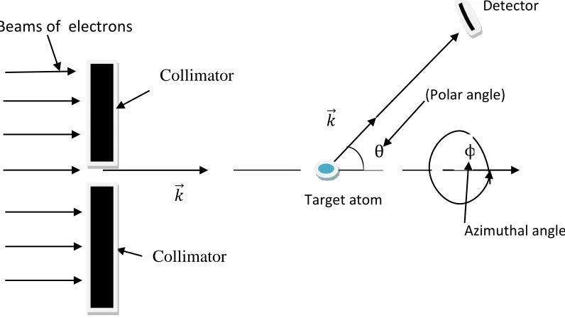
Figure 1.1: A diagram showing electron-atom scattering experiments ... 3
Figure 5.1: Differential cross sections at 10 eV. ... 46
Figure 5.2: Differential cross sections at 20 eV ... 47
Figure 5.3:. Differential cross sections at 30 eV. ... 48
Figure 5.4: Differential cross sections at 40 eV ... 49
Figure 5.5: Differential cross sections at 50 eV. ... 50
Figure 5.6: Differential cross sections at 70 eV ... 51
Figure 5.7: Differential cross sections at 80 eV.. ... 52
Figure 5.8: Differential cross sections at 100 eV ... 53
Figure5.9: Differential cross sections at 200 eV.. ... 54
ABBREVIATIONS, ACRONYMS AND SYMBOLS AES Auger-Electron Spectroscopy
CCC Convergent Close Coupling CC2 Two-State Close-Coupling CPB Coulomb Projected Born DCS Differential Cross Sections DHF Dirac-Hartree-Fock DW Distorted Wave
DZ Double Zeta wave functions
DWBA First-Order Distorted Wave Born Approximation DWBA1 e – H inelastic scattering Computer Program eV Electron Volt
FBA First Born Approximation ICS Integral Cross-Sections MCS Monte-Carlo Simulation
OMPM Optical Model Potential Method RHF Roothan Hatree Fock
RVP Relativistic Variable Phase Sr Strontium
XPS X-ray Photoelectron Spectroscopy Bohr radius
A Antisymmetrizing operator
f Direct amplitude Born approximation g Exchange amplitude G+ Total Green’s function
Hamiltonian of isolated atom Intial wave vector
Final wave vector Factor of normalization
T Kinetic energy operator of the projectile Transition matrix
Arbitrary distortion potential V Interaction potential
Spherical harmonics Total wave function
Atomic wave functions for initial and final state respectively Plane wave for an initial-state of the projectile
Ω Solid angle
ABSTRACT
CHAPTER ONE INTRODUCTION 1.1 Background to the study
Differential and integral cross sections for electron-atom are useful for interpretation and understanding of electron contact with the targets and deciding dynamics of the collision processes. Ramsauer (1921), conducted the first electron-atom scattering experiment and he made an observation that low energy elastic scattering with projectile energy of about 0.7eV by noble gas atoms full of transparency showed almost zero scattering. It contradicts classical mechanics which tries to determine a monotonic gain in the number of scattered electrons as falling electron energy diminishes. To investigate this, experiments on scattering have been carried out with various impact energies with different projectiles and target atoms for both elastic and in elastic processes. Cross-section data set for electron – atom elastic scattering are useful in X-ray photoelectron spectroscopy (XPS), upper atmosphere dynamics (Jablonski et al., 2004), Monte-Carlo simulation (MCS), Auger-electron spectroscopy (AES) (Jablonski
et al., 2004), in gaseous-exchange, laser development (McCarthy and Weigold, 1995),
plasma physics and fluorescent lighting. It is therefore evident that the knowledge of atomic collisions is important for calculations and also experimental approach in atomic physics.
scattering, energy is conserved after the interaction between the target and the projectile electron. In inelastic scattering energy is not conserved. After the interaction of the target and projectile electron, inelastic scattering results into positronium, ionization, target excitation or annihilation. (Ali and Soding, 1988).
Atomic collision study methods are further classified into two approaches either quantum mechanical approaches or semi-classical approaches. Quantum mechanical approaches are the one that uses the principle of quantum mechanics entirely; which is also classifieds into non-perturbative method and perturbative method. Examples of the non-perturbative methods are R-Matrix, the close coupling and other variational methods which employ the non-perturbative approach of close-coupling. The perturbative approaches are based on the expansion of the Born series or the distorted wave Born series. Examples of the perturbative methods are the eikonal series, the many-body theory, Born-Approximation and distorted wave born approximation (DWBA), While non-perturbative approaches are based on the close coupling approach that expands the test wave functions into a set of basic functions.
Semi - classical approaches borrows from both classical and quantum mechanics. Some of the examples of the methods are semi – classical impact parameter method, eikonal approximation, classical trajectory Monte Carlo method and Glauber Approximation.
θ ϕ
𝑘
𝑘
Collimator Collimator Beams of electrons
(Polar angle)
Azimuthal angle Target atom
single energy channel electrons of momentum falling on target atoms. After the interaction between the incident electron and target, the incident projectile electrons were then turned away from their initial course retaining their original energy. This phenomenon describes elastic scattering.
Detector
Figure 1.1: A diagram showing electron-atom scattering experiments
In the study of electron-atom scattering theory the main aim is to investigate the characteristic of electron-atom body in the asymptotic region. Many methods have been formulated for the computation of cross sections. These methods are the R-Matrix method (Burke and Berrington, 1993), the close-coupling (CC) method (McCarthy and Weigold, 1995) and the distorted-wave Born approximation (DWBA) (Joachain, 1975). R-matrix method is taken to be composed of more than one part through theory of atomic structure. In the CC approach, the wavefunction of the electron-atom system is expanded in terms of known target-atom states and unknown scattered-electron states.
Differential cross sections (DCS) in relation with integral cross sections (ICS) look at the feature of interaction potential and depends more on the target wave function and the estimated approach used in computation (Zhong et al., 1997). DCS for one scattering procedure if known with certainty can also be used to modify data belonging to different collisions processes (Scott and Taylor, 1979).
approximated and is treated as two electron system. The incident and scattered electrons continuum wave functions were calculated using staticpotential of the target.
1.2 Statement of research problem
For the intermediate energy region both differential and integral cross section for elastic scattering of electrons for strontium have been determined using first-order distorted wave Born approximation (DWBA) method in this study.
For elastic scattering of strontium very few calculations have been performed and currently there are no known results using the present method. Also the available theoretical results do not have other results to be compared with so it makes it important to obtain results to compare them and to be compared with future experimental results.
DWBA is a perturbative method which has been marked by favorable outcome; it is used to determine both differential and integral cross sections at intermediate and high incident energies for electron-atom collisions. Hence, DWBA at intermediate energy region 10eV to 200eV for elastic scattering of electron strontium and for scattering angles from 0o to 180o has been used in this study.
1.3 Rationale of study
study of differential and integral cross sections for elastic scattering of electron strontium was calculated using distorted wave method for a range of 10-200eV in an attempt of providing result for comparing with the only available theoretical differential cross section results in the range of 10-200eV (Adibzadeh and Theosodiou, 2004) which were obtained using optical potential scattering method.
1.4 Objectives
1.4.1 General objective
The general objective was to use the distorted wave Born approximation method (DWBA) to the elastic scattering of electrons by strontium atom at intermediate energies.
1.4.2 Specific objectives
i. To develop the DWBA applied to 𝑒− - Sr scattering.
ii. To make changes on the DWBA1 computer program for strontium. iii. To determine differential cross section (DCS) and integral cross section
(ICS) at impact energies 10-200eV for elastic scattering of electron-strontium.
CHAPTER TWO LITERATURE REVIEW
2.1 Experimental studies on electron- strontium elastic scattering
From the experimental data of Romanyuk et al. (1980) the total cross sections for strontium at low energies of 0.2 to 10eV was obtained using electron trap method in which a collision chamber was used as a collector of scattered electrons and the entire electron optical system was placed in a parallel magnetic field required for velocity selection of the electron monochromator and for collimation of electron beam.
The electrodes, whose potentials are close to the cathode potential, were mounted at the entrance to the collision chamber and at its exit. This formed a trap for the electrons that lose some of their energy due to change of their direction as a result of collision with an atom. The scattered electrons oscillate between these electrodes along the magnetic field until they settled in the collision chamber, thus the differential cross section were measured. Romanyuk et al. (1980) tabulated the values of DCS from their experiments which they used atomic beam modulation at low energies of 0.2–10 eV.
2.2 Theoretical studies on electron-strontium elastic scattering
approach to the many-body theory calculations (Gribakin et al,1991) give results for elastic e – Sr scattering and static- exchange plus parameter correlation- polarization potential calculations (Kumar et al,1994). Szmytkowski and Sienkiewicz (1994) calculated differential cross sections for elastic scattering of electron strontium at lower and intermediate energies of 0.2 to 100eV using relativistic polarized orbital approximation. By solving Dirac-Hartree-Fock (DHF) equations for isolated target, a static part of the projectile target interaction potential was generated and polarization potential by solving coupled DHF equations for the target by projectile and including only the dipole term in scattering calculation for polarization potential. Kelemen et al. (1995) have investigated elastic scattering of electron with strontium using phenomenological complex optical potential at impact energies less than or equal to 200eV. In the polarization potential, the values of adjustable variables were found using known electron attraction to the strontium atoms. Adibzadeh and Theosodiou (2004) used the optical potential method to calculate DCS at 10-200eV.
CHAPTER THREE
THEORIES OF ATOMIC COLLISION 3.1 Introduction to Approximation Methods in Atomic Collisions
It is difficult to obtain exact results for atomic collision cross sections, in most instances
the necessary atomic wave functions are not known exactly and the approximate wave
functions on which we must rely are frequently not orthogonal. Evidently, as the structural complexity of the colliding atoms increases, the difficulty of obtaining good wave functions also increases and more complex reactions become possible.
Calculations on molecular systems are particularly difficult. Furthermore, the structure of the equations to be solved is such that approximate methods must be used even if the
necessary wave functions are completely and exactly known (McDaniel, 1989).
Approximation methods to scattering can be basically classified into quantum
mechanical methods and semi-classical methods. In quantum mechanical methods,
concept of quantum mechanics are used fully. They are categorized into close coupling
methods and perturbative methods. Examples of perturbative methods are the distorted
wave series, Coulomb Projected Born approximations and the Born series while close
coupling methods include R-matrix and convergent close coupling.
In the semi-classical methods both quantum mechanics and classical mechanics are
used. Examples of these methods are classical trajectory Monte Carlo method, eikonal
3.2 Quantum Mechanical Approximations 3.2.1 The Born Approximation
In this approximation the amplitude is given as
⟨ | | ⟩ (3.1)
where U represents the interaction potential, = . 𝑒 is the product of final target
wave function and final plane wave of the projectile 𝑒 is the product of
initial atomic wave function and initial plane wave of the incident particle and is the
outgoing Green’s function written as
( )
(3.2)
From equation (3.1) the Born approximation to the amplitude are given as
⟨ | | ⟩ (3.3)
⟨ | | ⟩ (3.4)
so (3.5)
up to which is also obtained through the same procedure. Where up to is
the first Born approximation, second Born approximation up to nth Born approximation
respectively to the scattering amplitude.
3.2.2 Coulomb Projected Born (CPB) Approximation
the Hamiltonian a term
is included which is the electron – nucleus interaction term, as shown below
(3.6)
and
(3.7)
The transition matrix is written as
⟨ | | ⟩ (3.8)
where
( ) ( ) (3.9)
In equation (3.9) is the coulomb wave of the projectile electron in the field of the nuclear charge of the hydrogen atom while is the final atomic wave function. The CPB approximation is obtained from (3.9) by approximating as 𝑒 ( ) ( ). Hence the contribution of the electron-nucleus interaction has been taken into account through the coulomb wave , which is in the transition matrix.
3.2.3 Convergent Close Coupling (CCC) Method
CCC is applicable at all impact energies for both elastic and inelastic scattering. This
method depends mostly on close coupling to solve coupled equations with no
Resolving target Hamiltonian in an orthogonal Laguerre basis, target states are
determined for completeness to be reached as the basis size increases. In this method
the distinct and continuum parts of the target are treated through close coupling to allow
credibility of this method and independence of projectile energy (Fursa and Bray,
1995).
3.2.4 The Optical Model Potential Method (OMPM)
In this method elastic scattering of an atom is analyzed from a complicated target. The optical potential or pseudo potential replaces the difficult interactions for projectile and target particle in which the falling particle moves. After optical potential is calculated, the initial many body problems reduce to a single body. This potential is complex hence approximations are needed (Joachain, 1975).
3.2.5 The R-Matrix Method
chosen basis in the internal region and the cross sections calculated by solving the asymptotic problem in the external region (Burke, 2011).
3.2.6 The Distorted Wave Methods (DWM)
Distorted wave method was developed as a result of failures from first Born approximation (FBA). It works well since it is one of perturbative methods, the transition between final and initial elastic state is obtained and at high and intermediate energies, DCS for electron excitation of atoms are calculated (Itikawa, 1986). The distorted wave series converges faster than in Born series. DWM is more useful in the study of atom ionization, heavy particles collision processes among heavy particles and collision of electron molecules. It is more useful in interpreting excitation processes, the consequences of certain distortion potentials (Katiyar and Srivastava, 1988).
3.2.7 Distorted Wave Formula Using Two Potential Scattering Model
Let H be the total Hamilton of the projectile electron and N-electron target atom. Then we can write
(3.10)
where (3.11)
Therefore
where ∑
where V, T and , represents interaction potential, function for kinetic energy and Hamiltonian target respectively. In this case interaction potential is divided into two parts the approximate and the exact part. That is
V=U + W (3.13)
It is assumed that
(3.14)
where , can be evaluated exactly i.e. we are able to evaluate the Lippmann- Schwinger’s equation
(3.15)
where U is the distortion potential chosen in such a way that V - U = W, is a small perturbation and χ is the distorted wave corresponding to the free wave distorted by the availability of the distortion potential. E represents the system total energy. Where the subscripts (+) and (-) shows the outgoing and incoming wave boundary conditions respectively. For elastic scattering the transition matrix is written as
=
〈
〉
(3.16)
where is the total initial wave function and fulfills the Schroedinger equation
(3.17)
(3.18)
so that
(3.19)
where iis initial and f is final channel. From equation (3.18), can be written as
⟨ | | ⟩ (3.20)
Making use of the relation
(3.21)
we get
〈 〈 | - 〈
(3.22)
where we have taken into consideration the transition on the energy shell so that E= Ei= Ef
̅ (3.23) Now becomes
⟨ | | ⟩ ⟨ | | ⟩ ⟨ |
| ⟩ (3.24)
〉 〉
〉 (3.25)
Considering that on the energy shell
⟨ | | ⟩ = ⟨ | | ⟩ ⟨ | | ⟩ (3.26)
so (3.24) simplifies to
⟨ | | ⟩ ⟨ | | ⟩ (3.27)
The relation (3.26) is the two potential formulae of Gellman and Goldberger. The relation (3.27) is simplified once we assumes ; and
to
⟨ | | ⟩ ⟨ | | ⟩ (3.28)
By using the two potential scattering models the relation (3.28) is obtained which is the distorted wave formula. Here potential U distorts the wave function. When using the distorted wave method (3.28), U has to be determined first. It is the choice of this distortion potential that brings different forms of the distorted wave approaches.
3.2.8 The Bethe-Born Approximation
series of terms corresponding to the atomic transition moments is obtained (i.e. electric dipole, electric quadrupole)
3.3 Semi Classical Approximations 3.3.1The Glauber Approximation
Glauber et al (1959) while seeking a high energy scattering approximation more
satisfactory than the first Born approximation, proposed an Eikonal method, in which
all states of the perturbation expansion were added, with the leading term being the
Born approximation. The Glauber et al (1959) approximation was introduced for
nuclear problems and was not applied to atomic collision until 1968. However, it has
subsequently been used extensively in calculations on elastic and inelastic collisions of
electrons with atoms and molecules, at intermediate and high energies. One of its useful
features is that it satisfies the optical theorem, thereby being applicable in certain
situations where the potential is large for the Born approximation to be acceptable.
3.3.2 The Eikonal approximation
When the wavelength of the projectile is little comparably with the distance through
which the scattering potential varies to a noticeable degree, (Joachain, 1975), the study
of a classical trajectory gets meaning. If is the extent of the potential, the condition
can be stated as,
This condition is the basis of semi-classical scattering approximations, which have been
very useful for heavy particle, and also for electron, scattering. Further, if the energy of
the projectile, E, is large compared with a typical value of thepotential , so that
(3.30)
the Eikonal approach to scattering problems becomes feasible.
3.3.3 The Classical Trajectory Monte Carlo Method
This method provides a means of evaluating collision cross sections. The equations
governing the relative motion of the collision partners are integrated step by step on a
computer for a large number of different impact parameters. The final states of the
particles are determined, and the outcome of the collision is recorded. A Monte Carlo
method is used for random selection of the impact parameter and the relevant target
parameters (such as the position and momentum of the bound electrons). Thousands of
collisions are studiedand cross sections are determined from the relative probabilities of
the different values.
3.3.4 The Semi Classical Impact Parameter Method
Many cross section calculations on systems for which the concept of a well-defined
trajectory is valid for the relative motion have been made in the impact parameter
formulation. The trajectory is taken to be rectilinear, and the impact parameter plays the
role of angular momentum. Quantum mechanics is used to treat the electronic motion,
is to integrate numerically the classical equations of motion to obtain the trajectory, or
CHAPTER FOUR
MATERIALS AND METHODS 4.1 The distorted wave method (DWM)
There exist variants of DWM based on how the distortion for the electron wave has been introduced. The DWM was brought in due to the drawbacks experienced in the first Born approximation (FBA) (Madison and Bartschat, 1996). The FBA gave results in harmony with experimental data for the higher energies. This was realized using the plane waves for projectile electron; though it gave poor results for low impact energies and large angle differential cross sections, this necessitated the development of the Distorted Wave Method. In the DWM the plane wave is replaced by a distorted wave.
In the two – potential approach the T – matrix (as given in equation 3.28) for electron – atom (N – electron atom) scattering takes the following form (Madison and Bartschat, 1996) (where is replaced by the product of projectile and target wave functions and total wave function is written in antisymmetrized form)
( )⟨ ( ) ( )| | ( )⟩
⟨ ( )ϕ ( )| | ( ) ( )⟩ (4.1)
where are atomic wave functions for initial and final state respectively, 𝑒 ( ) is plane wave for an initial-state of the projectile and A is the operator for antisymmetrizing given by
where is the exchange operator between 0th and ith electron. Potential is a chosen distorting potential for the projectile, needed to determine the distorted wave by solving the wave equation
( ) (4.3)
using Numerov’s method ( Madison and Bartschat , 1996).
T and are the operator for kinetic energy of isolated projectile and the energy for final state of projectile respectively. For the total wave function in (4.1)
approximations are needed since it cannot be solved fully.
. Where is the atomic wave function (initial) and is distorted wave (initial). Then a power series expansion can be developedfor the
interaction, which is taken to be small. For energy Ei of the projectile electron, the initial state distorted wave is a solution of Schröedinger equation
( ) (4.4)
for chosen distortion Ui which diminishes asymptotically. Lippmann – Schwinger solution for the total wave function ( ) in terms of is written as
[ ( )] (4.5)
where G+ is given as
By putting a chosen potential U in equation (4.6), the distorted Green’s function g+ is written as
g+ =(E - Ha - T - U + i )-1 (4.7)
The total Green’s function G+ can be written using the distorted Green’s function g+ as
G+ = g++ G+ (V -U) g+ (4.8)
The full Green’s function series expansion can be written as
G+= g+ +G+ (V - U) g+ + G+ (V - U) g+ (V - U) g+ (4.9)
Ifequation (4.5) is put in (4.1) along with equation (4.9), we get
………… (4.10)
where
( )⟨ ( ) ( )| | ( ) ( )⟩
⟨ ( ) ( )| | ( ) ( )⟩ ( )
( )⟨ ( ) ( )|( ) ( )| ( ) ( )⟩ (4.12)
and
( )⟨ ( ) ( )|( ) ( ) ( )| ( ) ( )⟩
Equation (4.10) is the distorted wave series for the T- matrix while in this study the first order distorted wave approximation (4.11) was used. Direct and exchange transition matrices were determined from (4.11), where an atom has two valence electrons for elastic scattering, we get
(4.14)
with
⟨ ( ) ( )| | ( ) ( )⟩ (4.15)
and
⟨ ( ) ( )| | ( ) ( ) ( ) ( )⟩ (4.16)
In elastic scattering case the terms containing distorted waves in the direct T-matrix vanishes and one gets as given in equation (4.15). Neglecting the terms, with overlap integral between the bound and continuum states (which would be small at intermediate and high energies), we get as
⟨ ( ) ( )| | ( ) ( ) ( ) ( )⟩ (4.17)
The partial waves and are replaced in the transition matrices (4.15) and (4.17) to solve them (Madison and Bartschat (1996) and Singh (2004)).
〉 √ ∑ ( )
( ̂) ( ̂ ) (4.18)
〉 √ ∑ ( ) ( ̂) ( ̂ ) (4.19)
where is the spherical harmonic. In the expansion of the complex conjugate of the radial part is taken so that it satisfies the incoming wave boundary conditions. Substituting the above partial wave expansions of the distorted waves equations (4.18) and (4.19) into (4.20) and (4.21)) respectively,
( ) (4.20)
( ) (4.21)
where and are in Rydberg units. The radial distorted wave is a solution of the Schroedinger equation
( ( ) ( ) ) ( ) (4.22)
and it is solved by using the Numerov method (Madison and Bartschat, 1996). In the asymptotic region equation (4.22) take the form
( ) ( ) (4.23)
where is irregular and is regular Ricatti – Bessel functions and 𝑙 is a complex number given as
𝑒 ( ) (4.24)
4.2 Differential cross-section (DCS) and integral cross-section (ICS)
Differential cross section is the probability of finding scattered particles within a given solid angle, determined by the formula
[ ] (4.25)
By finding the integral of the differential cross section, integral cross section can be determined as
∫ ∫ ∫ 𝜃 ∫ 𝜃 (4.26)
4.3 Evaluation of Static Potentials
Even if the selection of the distortion potential is subject to individual discretion, the most used selection is the static potential at initial or final state, or both used together (Madison and Bartchat, 1996; Itikawa, 1986). It may also include polarization potential, absorption potential and exchange potential, in order to take account of polarization effects of the incident electron, absorption of particles and exchange effects from the incident channel respectively. Since it is the elastic scattering problem being
considered, both static potential and distortion potential are equal ( ).
⟨ϕ ϕ⟩ (4.27)
The interaction potential (V)
∑
where is the projectile electron atom and is the distance between the projectile and the ith atomic electron. Since the target atom is being considered as two-electron atom, in the above relation N = 2 for the present case. The relation of the static potentials is given as
⟨ ⟩ (4.29)
where is the final or initial state target wave function and V is the interaction between the target and the projectile. For the target states Hartee- Fock wave functions from Clementi and Roetti (1974) have been used. In these wave functions is summed over Slater type orbitals of the basis set as
〉 ∑ 〉 (4.30)
and
〈 ∑ 〈 (4.31)
Values of represent the expansion coefficients and are the Slater type orbitals of the basis set. Using equation (4.30) and (4.31) in equation (4.29), the distortion potential can be written as
∑ ∑ ⟨ | | ⟩ (4.32)
∑
(4.33)
(4.34)
The electron interaction potential
is expanded in terms of spherical harmonics
as
∑ ∑
( ) ( ) (4.35)
where r lesser ( ) or r greater ( ) of and . In the calculation, the interaction potential (V) have nuclear part on the right hand side of equation (4.34) plus the monopole term (𝑙 ) of the summation of equation (4.35). Because of the effects of the terms that are not spherical is negligible (Madison et al., 1996).
√ (4.36)
In Rydberg units the static potential is given as
∑ ∑ ⟨ | | ⟩
∑ ∑ ⟨ | | ⟩ (4.37)
The radial wave functions and spherical harmonics their product gives the slates type orbitals (Clementi and Roetti, 1974) written as
( )
( ̂) (4.38)
( )
√( ) (4.39)
Substituting the wave function in equation (4.38) putting standard integral to replace Bra and Ket notation, this gives a fully extended static potential as shown
∑ ∑ ∫ ( )(
) 𝑒 ( [ ] ) ∫ ( ) ( )
In equation (4.40) above, partial integration from radial distance 0 to , is taken to be larger than and from 𝑜 , is taken to be larger than . The right hand side of equation (4.40) vanishes as a result of spherical harmonics being orthonormal unless 𝑙 𝑙 and .
Resulting to
∑ ∑ ∫ ( ) 𝑒 ( ) (4.41)
where k =[ ]
In this study, the exact static potentials were obtained by solving this integral in order to get the distortion potentials. The total static potential is the addition of elements in matrix.
The solutions the equation (4.41) changes according to the sum of the principal
quantum numbers . This sum changes from (4.50) to (4.58) for the problem that was determined as follows.
The following procedure was followed to determine distortion potential
For r2 ⟨ ( ̅ ) ( ̅ )|
| ( ̅) ( ̅ )⟩ (4.42)
The term associated with
gave
⟨ ( ̅ )|
| ( ̅)⟩ (4.43)
The term associated with
gave
⟨ ( ̅ )|
| ( ̅ )⟩ (4.44)
and the term associated gave
⟨ ( ̅ ) ( ̅ )| | ( ̅) ( ̅ )⟩ ⟨ ( ̅ )| | ( ̅)⟩ (4.45)
in Rydberg units.
Combining (4.43), (4.44), and (4.45), we get
∫ ( ) = (∫ ( ) ∫ ( ) dr) (4.46)
∫ 𝑒 ( ) ∫ ( ) ∫ ( )
=∫ ( ) ∫ ( ) (4.47)
Considering the first term of equation (4.47) above
∫ ( ) ( ) * ∫ ( ) +
= ( ) [ ( ]
= 𝑒 ( ) ( ) (4.48)
Now considering the second term of equation (4.47) it can be seen that
∫ 𝑒 ( ) ( 𝑒 ( ) ∫ 𝑒 ( ) )
= ( 𝑒 ( ) * 𝑒 ( ) 𝑒 ( )+)
= ( 𝑒 ( ) 𝑒 ( ) 𝑒 ( ) )
=( 𝑒 ( ) 𝑒 ( ) 𝑒 ( ) (4.49)
Therefore using equation (4.48) and (4.49) leads to
∫ 𝑒 ( )( ) 𝑒 ( ) * ( ) ( )+
This is converted to computer code using fortran language as:
19 POT=POT+ANCO*(-EXP (-SETA*R)*(1./SETA**2+2./ (SETA**3*R)))
Similarly
For
∫ ( ) ( ) 𝑒 ( ) * ( ) ( ) ( )+
= 𝑒 ( ) * + (4.51)
This is converted to computer code using fortran language as:
29 POT=POT+ANCO*(-EXP (-SETA*R)*(R/SETA**2+4./SETA**3+ +6. / (SETA**4*R)))
For
∫ 𝑒 ( ) ( ) 𝑒 ( ) * ( ) ( )
( ) ( )+
= 𝑒 ( ) * + (4.52)
This is converted to computer code using fortran language as:
For
∫ 𝑒 ( ) ( ) 𝑒 ( ) * ( ) ( )
( ) ( )+
= 𝑒 ( ) * + (4.53)
This is converted to computer code using fortran language as:
49 POT=POT+ANCO*(-EXP (-SETA*R)*(R3/SETA**2+8*R*R/SETA**3+ 36*R/SETA**4+96./SETA**5+120./ (SETA**6*R)))
For
∫ 𝑒 ( ) ( ) =
𝑒 ( ) [ ( ) ( ) ( )
( ) ( )
( )]
𝑒 ( ) * + (4.54)
This is converted to computer code using fortran language as:
For
∫ 𝑒 ( ) ( )
𝑒 ( ) [ ( ) ( ) ( )
( ) ( )
( ) ( )]
𝑒 ( ) * + (4.55)
This is converted to computer code using fortran language as:
69 POT=POT+ANCO*(-EXP (-SETA*R)*(R5/SETA**2+12*R4/SETA**3+
90*R3/SETA**4+480*R*R/SETA**5+1800*R/SETA**6+4320./SETA**7+5040./ (SETA**8*R)))
For
∫ 𝑒 ( ) ( )
𝑒 ( ) [ ( ) ( ) ( )
( ) ( )
( ) ( )
𝑒 ( ) * + (4.56)
This is converted to computer code using fortran language as:
79 POT=POT+ANCO*(-EXP (-SETA*R)*(R6/SETA**2+14*R5/SETA**3+
126*R4/SETA**4+840*R3/SETA**5+4200*R*R/SETA**6+15120*R/SETA**7+352 80./SETA**8+40320./ (SETA**9*R)))
For
∫ 𝑒 ( ) ( )
𝑒 ( ) [ ( ) ( ) ( )
( ) ( )
( ) ( )
( ) ( )]
𝑒 ( ) *
+ (4.57)
This is converted to computer code using fortran language as:
168*R5/SETA**4+1344*R4/SETA**5+8400*R3/SETA**6+40320*R*R/SETA**7+1 41120*R/ SETA**8+322560./SETA**9+362880./ (SETA**10*R)))
And finally
For
∫ ( ) ( )
( ) ⌊ ( ) ( ) ( )
( ) ( )
( ) ( )
( )
( )
( )⌋
𝑒 ( ) *
+ (4.58)
This is converted to computer code using fortran language as:
216*R6/SETA**4+2016*R5/SETA**5+15120*R4/SETA**6+90720*R3/SETA**7+4 23360*R*R/SETA**8+1451520*R/SETA**9+3265920./SETA**10
+3628800./(SETA**11*R)))
The values of and ANCOi are determined from from Clementi and Roetti (1974) table. This helped to make changes on computer program which develop the needed static potential.
The normalization factor N and the expansion coefficient C are the values that makes ANCOi and all is from Clementi and Roetti (1974) tables.
4.4 ANCO values for the distortion potential elements 5s state For term with
ANCO =
For term with
ANCO =
For the term with
ANCO =
For term with
ANCO =
For term with
ANCO =
For term with
ANCO =
For the term with
ANCO =
For the term with
ANCO = For the term with
ANCO =
All static potential elements are summed up to get (the static potential for initial, s=i
4.5 Computer Program DWBA1
Table 4.1: Input file for e-Sr scattering at 200 eV
4.6 Atomic Wave Functions
Roothan Hartree Fock (RHF) atomic wave function have been used obtained from Clementi and Roetti (1974) table in which the radial orbital ( ) are expressed as,
( ) ∑ ( ) (4.59)
where ( ) are normalized Slater- Type Orbitals (STOs).
The full wave function is written as
1,0,1,0,200, NI LI NF LF ENERGY
-1,1 PROJECTILE CHARGE, TARGET CHARGE
1, 0 INIT. STATE STAT. POT. (N L; 0, 0 = PLANE WAVE) 1, 0 FINAL STATE STAT. POT. (N L; 0,0 = PLANE WAVE) 1.E-6,1.E-6,1.E-4,1.E-4 WF ZERO, FORM RATIO ZERO, EXCHANGE RATIO ZERO 6,15,20,25,55,60,65 # PRINT FLAGS, PRINT FLAGS
0,0,0,0,0,16 TAPE UNITS FOR INPUT AND OUTPUT 10 NN
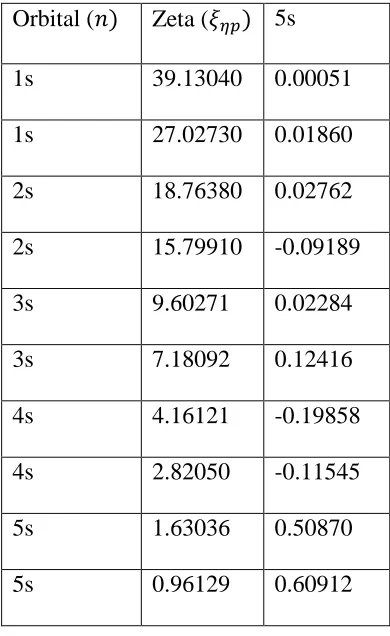
39.13040,27.02730,18.76380,15.79910,9.60271,7.18092,4.16121,2.82050,1.63036,0.96129 ZETA
0.00051, 0.01860, 0.02762,-0.09189,0.02284,0.12416,-0.19858,-0.11545,0.50870,0.60912 COEFFICIENT
( ( ) ( )) (4.60)
where represent spin orbital, n represent total number of electrons and A represent antisymmetrizing operator, assumption is made that they are all mutually perpendicular.
The orbital ϕ is written as
ϕ ∑ (4.61)
where is the basis functions, p is basis function with correspondence to and C is constant of expansion.
The is the basis functions given as
( 𝜃 ) ( ) (𝜃 ) (4.62)
The radial part is written as;
( ) 𝑒 (4.63)
The factor of normalization N is given as
(( ) ) ( ) (4.64)
Table 4.2: Values from K(2)L(8)M(18)4S(2)4P(6)5S(2),1S of strontium. T.E. = -0.313146552D+04, P.E. = -0.626306960D+04, K.E.= 0.3136044D+04, V.T.=-0.19999556D+01 in atomic units.
Orbital ( ) Zeta ( ) 5s 1s 39.13040 0.00051 1s 27.02730 0.01860 2s 18.76380 0.02762 2s 15.79910 -0.09189 3s 9.60271 0.02284 3s 7.18092 0.12416 4s 4.16121 -0.19858 4s 2.82050 -0.11545 5s 1.63036 0.50870 5s 0.96129 0.60912
The double- zeta type wave functions for strontium are given as:
( ) ∑
( )
where
( ) (𝜃 ) (4.65)
( ) (𝜃 ) (4.66)
( ) (𝜃 ) (4.67)
( ) (𝜃 ) (4.68)
( ) (𝜃 ) (4.69)
( ) (𝜃 ) (4.70)
( ) (𝜃 ) (4.71)
( ) (𝜃 ) (4.72)
( ) (𝜃 ) (4.73)
( ) (𝜃 ) (4.74) converted in computer code using fortran language as
PHI(I)=AN(I)*X**K*EXP(-ZETA(I)*X
and the factors for normalization are written as in equation (4.64) where is principal quantum number is orbital exponents and are written as given in ANCO values for the distortion potential elements 5s state above.
Wave function of double zeta is obtained by adding all the basis functions from Clementi and Roetti table for the radial part. These are based on Roothan – Hartee – Focks (RHF) expansion technique.
4.7 Normalization
For normalization, the equation below must hold
∫ (4.75) However
∫ (4.76) where is constant of expansion.
Then we performed the following operation to achieve normalization. Divide the final potent calculation by the factor k, i.e. potent and subsequently divide the atomic wave function [UU(J)] by the square root of k i.e. UU(J) / SQRT (k). Where UU(J) is the wave function.
4.8 Computer code
CHAPTER FIVE RESULTS DISCUSSIONS 5.1 Introduction
At intermediate energies differential cross section results for elastic scattering of electron by strontium have been obtained in this study and these will be discussed in part 5.2. At the impact energies 10, 20, 30, 40, 50, 70, 80, 100 and 200eV, differential cross sections (DCS) results are calculated and tabulated as shown in table 5.1. The integral cross section results obtained by DWBA are represented and comparisons done with the only available theoretical results by Adibzadeh and Theosodiou (2004). There are no experimental DCS results to be compared with.
5.2 Differential cross sections
At 10, 20, 30, 40, 50, 70, 80, 100 and 200 eV differential cross section (DCS) are
calculated using DWBA by a strontium atom with scattering angles ranging from 0° to
180° and present results tabulated in table 5.1 below and plotted as shown in figures 5.1
to 5.9 and comparing it with calculated results of Adibzadeh and Theosodiou (2004),
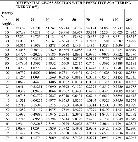
Table 5.1: Differential cross sections calculated for the elastic scattering of electrons from strontium atom (in units of ).
DIFFERNTIAL CROSS SECTION WITH RESPECTIVE SCATTERING ENERGY (eV)
Angles
10 20 30 40 50 70 80 100 200
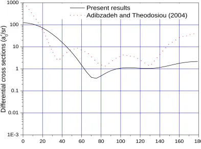
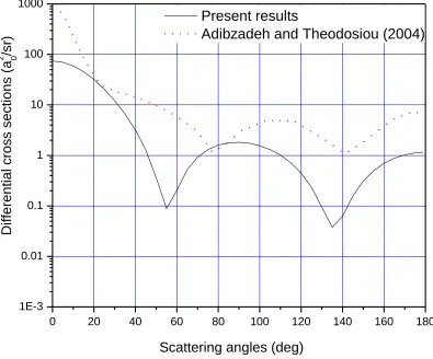
Figure 5.1: Graph of differential cross sections against scattering angles at incident energy of 10 eV for a strontium atom. Present results, Adibzadeh and Theodosiou (2004).
From figure 5.1, differential cross sections at 10 eV for present results disagree with the
Adibzadeh and Theodosiou (2004) theoretical results. The present results have two
minima at 70° and 130° (at 1300 it is very shallow) whereas calculated results of
Adibzadeh and Theodosiou (2004) using optical potential method have three minima at
around 350, 850 and 1300. But the values of the cross sections for both the cases are in
the same range. The disagreement could be because DWBA does not work well at
lower impact energies and also the nature of the distortion potential used in this method.
0 20 40 60 80 100 120 140 160 180
1E-3 0.01 0.1 1 10 100 1000 Present results
Adibzadeh and Theodosiou (2004)
Scattering angles (deg)
D iff e re n tia l cro ss se ct io n s (a
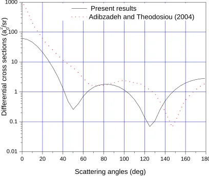
Figure 5.2: Graph of differential cross sections against scattering angles at incident energy of 20 eV for a strontium atom. Present results, Adibzadeh and Theodosiou (2004).
From figure 5.2, it shows that the present results disagree with the results of Adibzadeh
and Theodosiou (2004). The present results had two minima at 450 and 135° whereas
results of Adibzadeh and Theodosiou (2004) had two minima at 750 and 1400 which
were shifted to the right with respect to the present minima positions. It can be said that
the two results agree qualitatively (since both have two minima) but disagree
quantitatively. The discrepancy can also be attributed to the difference in the distorting potential between the two methods.
0 20 40 60 80 100 120 140 160 180
1E-3 0.01 0.1 1 10 100 1000 Present results
Adibzadeh and Theodosiou (2004)
Scattering angles (deg)
D if fe re n ti a l cro ss se ct io n s (a
Figure 5.3: Graph of differential cross sections against scattering angles at incident energy of 30 eV for a strontium atom. Present results, Adibzadeh and Theodosiou (2004).
In figure 5.3, it was seen that at 30 eV the present results agree qualitatively since the present result has two minima at 500 and 1250 and that of Adibzadeh and Theodosiou
(2004) has also two minima at 650 and 1500 which are shifted to the right. Though both
results seem to disagree quantitatively, both lie within the same range of values.
0 20 40 60 80 100 120 140 160 180
0.01 0.1 1 10 100 1000
Scattering angles (deg)
D
if
fe
re
n
ti
a
l
cro
ss
se
ct
io
n
s
(a
2
/sr)
0Present results
Figure 5.4: Graph of differential cross sections against scattering angles at incident energy of 40 eV for by a strontium atom. Present results, Adibzadeh and Theodosiou (2004).
From figure 5.4, the present result has two minima at 450 and 1200 whereas the result of Adibzadeh and Theodosiou (2004) has minima at 600 and 1450. The present results agree well qualitatively and quantitatively with results of Adibzadeh and Theodosiou
(2004) below 1200 compared to what it was at lower energies.
0 20 40 60 80 100 120 140 160 180
1E-4 1E-3 0.01 0.1 1 10 100 1000 Present results
Adibzadeh and Theodosiou (2004)
Scattering angles (deg)
D if fe re n ti a l cro ss se ct io n s (a
Figure 5.5: Graph of differential cross sections against scattering angles at incident energy of 50 eV for a strontium atom. Present results, Adibzadeh and Theodosiou (2004).
From figure 5.5, the present result has two minima at 500 and 1150 just like calculated results of Adibzadeh and Theodosiou (2004) which has minima at 550 and 1350. It is only that the second minimum of the current results is shifted to the left. The present results agree qualitatively and quantitatively with theoretical results of Adibzadeh and
Theodosiou (2004) compared to the agreement at lower energies.
0 20 40 60 80 100 120 140 160 180
1E-3 0.01 0.1 1 10 100 1000 Present results
Adibzadeh and Theodosiou (2004)
Scattering angles (deg)
D if fe re n ti a l cro ss se ct io n s (a
Figure 5.6: Graph of differential cross sections against scattering angles at incident energy of 70 eV for a strontium atom. Present results, Adibzadeh and Theodosiou (2004).
From figure 5.6, the present result again has two minima at 450 and 1100 and that of Adibzadeh and Theodosiou (2004) has two minima at 500 and 1100.The present results agree well qualitatively and quantitatively with theoretical results of Adibzadeh and
Theodosiou (2004) compared to the agreement at lower energies.
0 20 40 60 80 100 120 140 160 180
1E-3 0.01 0.1 1 10 100 1000 Present results
Adibzadeh and Theodosiou (2004)
Scattering angles (deg)
D if fe re n ti a l cro ss se ct io n s (a
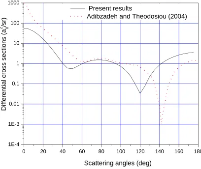
Figure 5.7: Graph of differential cross sections against scattering angles at incident energy of 80 eV for a strontium atom. Present results, Adibzadeh and Theodosiou (2004).
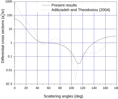
From figure 5.7, the present result has one minimum at 1100 and that of Adibzadeh and
Theodosiou (2004) has three minima at 450, 1050 and 1500. The present results disagree
qualitatively with those of Adibzadeh and Theodosiou (2004), even if the DCS are within the same range.
0 20 40 60 80 100 120 140 160 180
1E-3 0.01 0.1 1 10 100 1000
Scattering angles (deg)
D if fe re n ti a l cro ss se ct io n s (a
2 /sr) 0
Present results
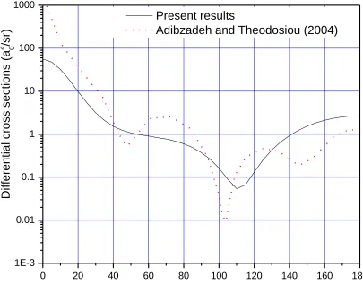
Figure 5.8: Graph of differential cross sections against scattering angles at incident energy of 100 eV for a strontium atom. Present results, Adibzadeh and Theodosiou (2004).
From figure 5.8, the behaviors of these results are the same as at 80eV. The present result has one minimum at 1100 and that of Adibzadeh and Theodosiou (2004) had three minima at 450, 950 and 1500.The two results disagree qualitatively though they are in the same range.
0 20 40 60 80 100 120 140 160 180
1E-3 0.01 0.1 1 10 100 1000 Present results
Adibzadeh and Theodosiou (2004)
Scattering angles (deg)
D if fe re n ti a l cro ss se ct io n s (a
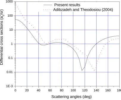
Figure5.9: Graph of differential cross sections against scattering angles at incident energy of 200 eV for a strontium atom. Present results, Adibzadeh and Theodosiou (2004).
From figure 5.9, the present result has two shallow minima at 700 and 1300 and that of Adibzadeh and Theodosiou (2004) has minima at 400, 850 and 1450. The mimimum at 850 is very deep. The present results disagree qualitatively with the results of Adibzadeh
and Theodosiou (2004). But except for a sharp minimum at 850 for the Adibzadeh and
Theodosiou (2004), both results seem to lie within the same range.
0 20 40 60 80 100 120 140 160 180
1E-4 1E-3 0.01 0.1 1 10 100 1000
Scattering angles (deg)
D
if
fe
re
n
ti
a
l
cro
ss
se
ct
io
n
s
(a
2
/sr)
0Present results
Though the present results disagree qualitatively and quantitatively agree well to Adibzadeh and Theodosiou (2004), both results are almost at all scattering angles and at all impact energies in the same range. The minima represent the direction in which the
electrons are least likely to be deflected while the maxima represent the direction to
which the electrons are most likely to be deflected. It can be concluded from figures
5.1-5.9, that the present DWBA calculated results are reliable for differential cross sections at the intermediate energies. The difference between the present results and the results of Adibzadeh and Theodosiou (2004) is because present DWBA has only considered a restricted form of static potential as the distortion potential whereas for the Adibzadeh and Theodosiou (2004) they have included static, exchange and polarization potentials this cause the main discrepancies at lower angles since polarization potential has a great effect at lower angles.
5.3 Integral cross sections
Table 5.2: Integral Cross Section results (in units of ) calculated for the elastic scattering of electrons by strontium atom.
Energy Present
Adibzadeh and Theodosiou
(2004)
Kumar et al (1995)
Kelemen et al (1995)
10 96.51 196 96.6 145
20 42.37 138 43.5 104
30 32.75 123 25.93
40 28.34
50 25.55 99.3 13.5 62
60 23.55
70 22
80 20.73 90 19.67
100 18.75 66.9 8.53 39
110 17.93 59.9
120 17.21 130 16.56 140 15.98
150 15.44 49.3 7.4 29
160 14.95 170 14.49 180 14.07 190 13.68
200 13.32 40.56 6.4 25
Figure 5.10: Graph of integral cross sections against electron energy for a
strontium atom. present values of DWM, Kumar et al (1994), Kelemen et al (1995) and Adibzadeh and Theosodiu (2004).
It can be seen from figure 5.10 that the pattern of all the results are the same. At low energies the integral cross section is high and decreases with increase of the impact energy since the interaction time for the target atom and incident electrons reduces as the impact energy is increased. The present result is almost the same to that of Kumar et al (1994) where he used real potential.
In the absence of any experimental result it is hard to say which is better than the other.
0 20 40 60 80 100 120 140 160 180 200
0 20 40 60 80 100 120 140 160 180 200 220 Present results
Adibzadeh and Theodosiou(2004) Kumar et al (1994)
Kelemen et al (1995)
Electron energy(eV)
In
te
g
ra
l
cro
ss
se
ct
io
n
s
(a
CHAPTER 6
CONCLUSIONS AND RECOMMENDATIONS 6.1 Introduction
Using the first-order distorted wave Born approximation (DWBA) method differential cross sections (DCS) and Integral cross sections (ICS) have been calculated for elastic scattering of electron strontium atom scattering at intermediate energies. In the initial state of strontium atom both initial and final channel distortion potentials were taken as static potential. Double zeta Roothan-Hartree-Fock wave functions were used in the calculations as wave functions for the strontium atom as compiled by Clementi and Roetti (1974).
6.2 Conclusions
From this study the following observations were made:
i. The DWBA was developed and applied to 𝑒− - Sr scattering.
ii. Changes on the DWBA1 computer program were made for strontium.
iii. Differential cross section (DCS) and integral cross section (ICS) at impact energies 10-200eV for elastic scattering of electron-strontium were determined. iv. At energies between 10-30 eV, the present DCS results disagree with the only
available calculated results of Adibzadeh and Theodosiou (2004) for differential
cross section. This is because the first order distorted wave method gave poor
v. At energies of 60-200 eV, the present DCS results agreed well with calculated results of of Adibzadeh and Theodosiou (2004) though at 200eV the agreement is not so good.
vi. The integral cross section (ICS) graph structure for the present results agreed
well qualitatively with theoretical results of Kumar et al (1994), Kelemen et al
(1995) and Adbizadeh and Theodosiou (2004). Quantitatively, it is in better
agreement with Kumar et al (1994) result compared to Kelemen et al (1995) and
Adibzadeh and Theodosiou (2004).
vii. The present DWBA can be used to calculate DCS and ICS at intermediate energies.
6.3 Recommendations
From the results of DWBA using elastic scattering of electrons by strontium atom the following were recommended:
i. Some experimental studies on electron impact elastic scattering of strontium should be made to give results for comparison with the calculated results.
ii. Theoretical studies using close-coupling and R-matrix methods should be conducted on DCS for purposes of comparison with the present results.
iii. A distortion potential that incorporates the polarization potential, exchange potential and absorption potential should be used in the calculation.
REFERENCES
Ali, A. and Soding, P. (1988). High Energy Electron-Positron Physics. World Scientific Publishing Co Pte Ltd (Singapore) pp 790-793.
Adibzadeh, M. and Theodosiou, C.E. (2004). Elastic Electron Scattering from Ba and
Sr.Physical review A 70: 052704
Bartschat, K. and Sadeghpour, H.R. (2003). Ultralow-Energy Electron Scattering from Alkaline-Earth Atoms: the Scattering-Length Limit. Journal of Physics B: Atomic.
Molecular and Optical Physics 36: L9–L15.
Bethe, H.A. (1939). Energy Production in Stars. Physical Review 55:434-456.
Burke, P.G., Hibbert, A. and Robb, W.D. (1971). Electron Scattering by Complex Atoms. Journal of Physics B 4: 153-161
Burke, P.G. (2011). In R – Matrix Theory of Atomic collisions. Applications to Atomic,
Molecular and Optical Processes. (Springer, London) pp 3 – 15.
Clementi, E. and Roetti, C. (1974). Roothan – Hartree – Fork Atomic Wave Functions: Basis Functions and their Coefficients for Ground and Certain Excited States of Neutral and Ionized Atoms, Z ≤ 54. Atomic Data and Nuclear Data Tables 14: 177 – 478.
Fabrikant I. I., (1980) .Journal of Physics B: Atomic and Molecular Physics 13: 603-612
Fursa, V.D. and Bray, I. (1995). Calculation of electron-helium scattering. Physical
review A 52: 1279-1297.
Glauber, R.J., Brittin, W.E. and Dunham, L.B. (1959). Lectures in Theoretical Physics.
Interscience Publisher, Inc. Newyork. Vol. 1, pp 315
Gribakin G.F., Ivanov, V.K. and Kuchiev, M.Y. (1991). Physics of Electronic and
Atomic Collisions vol 12 (St Petersburg: FTI) pp 77-88 (in Russian)
Itikawa, Y. (1986). Distorted-Wave Methods in Electron-Impact Excitation of Atoms and Ions. Physics report 143:69-108.
Jabloski, A., Salvat, F. and Powell, C.J. (2004). Comparison of Electron–Elastic– Scattering Cross Sections Calculated from Two Commonly used Atomic Potentials.
Journal of Physical Chemistry 33: 409 – 451.
Joachain, C.J. (1975). Quantum Collision Theory. (North-Holland, Amsterdam). pp 576-621.
Katiyar, A. K. and Srivastava, R. (1988). Distorted – wave calculation of the cross sections and correlation parameters for e+ - He collision. Physical Review A 38:2767-2781.
Kelemen, V. I., Remeta, E. Y. and Sabad, E. P. (1995). Scattering of Electrons by Ca, Sr, Ba and Yb Atoms in the 0-200 eV Energy Region in the Optical Potential Model.
Journal of Physics B: Atomic, molecular and optical physics 28: 1527-1546.
Kumar, P., Jain, A.K., Tripathi, A.N. and Sultana N. Z. (1994) Journal of physics D
30:149
Madison, D. H. and Bartschat, K. (1996). The Distorted Wave Method for Elastic Scattering and Atomic Excitation, in Computation Atomic Physics. Ed. K. Bartschart. Springer-Verlag Berlin.
Madison, D.H. and Winters, K.H. (1983). A second order distorted wave model for the excitation of the 2 lp state of helium by electron and positron impact. Journal of Physics
B: Atomic, molecular and optical physics 16: 4437-4450.
McCarthy, I.E. and Weigold, E. (1995). In Electron – Atom Collisions. (Cambridge University Press, Cambridge). pp 156 – 190.
Mott, N.F. and Massey, H.S.W. (1965). The Theory of Atomic Collisions (Oxford University Press, New York).
Romanyuk, N.I., Shpenik, O.B. and Zapesochnyi, I.P. (1980). Cross Sections and Characteristics of Electron Scattering by Calcium, Strontium and Barium Atoms.
Journal of Experimental and Theoretical Physics Letters 32: 472-475.
Scott, T and Taylor, H.S. (1979). Elastic electron-helium scattering II. Application of many body theory. Journal of physics B. Atomic Molecular and Optical Physics. 12:3385-3397.
Singh, C.S. (2005). Electron Impact Excitation of 21S State Helium Atom. East African
Journal of Physical Sciences 6:67-77.
Singh, C.S. (2004). A study of Angular Correlation Parameters using a Distorted Wave Method. East African Journal of Physical Sciences 5: 25-30.
Szmytkowski, R. and Sienkiewicz, J. E. (1994). Elastic Scattering of Electrons by Strontium and Barium atoms. Physics Review A 50:80-952.
Yuan, J. and Zhang, Z. (1990). Alternative Static-Exchange Formalism: Low-Energy Electron Scattering with Heavy Alkaline-Earth Atoms. Physical Review A 42: 5363-5372
Zhong, Z.P., Feng, R.F., Wu, S.L., Zhu, L.F., Zhang, X.J., and Xu, K.Z. (1997). Electron- impact study for the 31S and n1P (n=3-6) excitations in helium. Journal of