Western University Western University
Scholarship@Western
Scholarship@Western
Electronic Thesis and Dissertation Repository
8-20-2018 2:30 PM
Vibrating-wire Rheometry
Vibrating-wire Rheometry
Cameron C. Hopkins
The University of Western Ontario
Supervisor de Bruyn, John R.
The University of Western Ontario Graduate Program in Physics
A thesis submitted in partial fulfillment of the requirements for the degree in Doctor of Philosophy
© Cameron C. Hopkins 2018
Follow this and additional works at: https://ir.lib.uwo.ca/etd
Part of the Statistical, Nonlinear, and Soft Matter Physics Commons
Recommended Citation Recommended Citation
Hopkins, Cameron C., "Vibrating-wire Rheometry" (2018). Electronic Thesis and Dissertation Repository. 5584.
https://ir.lib.uwo.ca/etd/5584
This Dissertation/Thesis is brought to you for free and open access by Scholarship@Western. It has been accepted for inclusion in Electronic Thesis and Dissertation Repository by an authorized administrator of
Abstract
This thesis consists of two projects on the behaviour of a novel vibrating-wire rheometer
and a third project studying the gelation dynamics of aqueous solutions of Pluronic F127. In
the first study, we use COMSOL to perform two-dimensional simulations of the oscillations of
a wire in Newtonian and shear-thinning fluids. Our results show that the resonant behaviour of
the wire agrees well with the theory of a wire vibrating in Newtonian fluids. In shear-thinning
fluids, we find resonant behaviour similar to that in Newtonian fluids. In addition, we find that
the shear-rate and viscosity in the fluid vary significantly in both space and time. We find that
the resonant behaviour of the wire can be well described by the theory of a wire vibrating in a
Newtonian fluid if the viscosity in the theory is set equal to the viscosity averaged over the
cir-cumference of the wire and over one period of the wire’s oscillation at the resonant frequency.
In the second study, we present the design and operation of our vibrating-wire rheometer and
use it to measure the properties of Newtonian and viscoelastic fluids. We find that our
de-vice can accurately measure small viscosities. In homogeneous polymer solutions, we find
that the viscoelastic moduli measured using our device are consistent with measurements at
lower frequencies using a shear rheometer. In addition, we find that our device can measure
the microrheological properties of an aging Laponite clay suspension that is heterogeneous on
the micron scale. In the third project, we study the gelation dynamics of aqueous solutions of
Pluronic F127. Using shear rheometry we find that when slowly heating the solutions, they
un-dergo a transition from sol to gel around room temperature, followed by a gel to sol transition
at a higher temperature. Our results show that these transitions take place over a temperature
range of a few degrees. When cooling the solutions, the reverse transitions occur over a larger
range of temperature and the width in temperature of the gel phase is larger. At temperatures
near the phase transitions, we find that the rheological relaxation time becomes very long.
Keywords: Rheology, rheometry, viscometry, vibrating wire, complex fluids, Pluronic,
COMSOL
Co-Authorship Statement
Chapter 2 has been published as: Cameron C. Hopkins and John R. de Bruyn, Vibrating
Wire Rheometry, Journal of Non-Newtonian Fluid Mechanics, 238, 2016. I did all of the
experiments, data analysis and writing of early drafts of the paper. John R. de Bruyn supervised
the project and provided editorial comments on the paper.
A version of chapter 3 is being prepared for submission. I did all of the simulations, data
analysis, and writing of the early drafts of the paper. John R. de Bruyn supervised the project
and provided editorial comments.
A version of chapter 4 will be submitted for publication in theJournal of Rheology. I did
all of the experiments, data analysis, and writing of the early drafts of the paper. John R. de
Bruyn supervised the project and provided editorial comments.
Acknowledgments
First, I must thank my advisor, Dr. John R. de Bruyn. I have grown considerably, both
personally and professionally, over my time here in no small part thanks to his mentorship and
patience. His guidance over the years has shaped me into an effective scientist. I feel like I am well prepared for a future in science thanks to him.
I gratefully acknowledge the funding received towards my PhD from the National Sciences
and Engineering Research Council, Ontario Graduate Scholarship, University of Western
On-tario, and the Canada Foundation for Innovation.
The work in chapter 3 was made possible by the facilities of the Shared Hierarchical
Aca-demic Research Computing Network (SHARCNET:www.sharcnet.ca) and Compute/Calcul Canada, and the provision of the COMSOL Multiphysics license by CMC Microsystems.
I am grateful for the guidance my advisory committee, Dr. Silvia Mittler and Dr. Michael
G. Cottom, have given me over the years.
Frank Van Sas and Brian Dalrymple manufactured the parts for my vibrating-wire
rheome-ter, and Doug Hie helped develop the electronics. Without their expertise this project would
not have been possible.
I want to thank fellow graduate student Nirosh Getangama, and former colleagues Yang
Liu and Masha Goiko, for their helpful discussions over the course of my PhD.
Thank you to my parents and brother for their unconditional support and encouragement
over the duration of my studies.
Finally, I must thank my wife, Ellie, for her unwavering support and patience over the last
year. I would not have been able to do this without her.
Contents
Abstract i
Co-Authorship Statement iii
Acknowledgements iv
List of Figures viii
List of Tables xviii
List of Symbols xix
List of Abbreviations xxi
1 Introduction 1
1.1 Fluids . . . 1
1.1.1 Shear Thinning and Shear Thickening . . . 3
1.1.2 Yield Stress . . . 5
1.1.3 Viscoelasticity . . . 7
1.1.4 Small-Amplitude Oscillatory Shear . . . 8
1.1.5 Shear Rheometry . . . 11
1.2 Summary of Present Work . . . 12
1.2.1 Overview . . . 12
1.2.2 Numerical Simulations of the Forced Oscillations of a Wire in a Fluid . 13
1.2.3 Vibrating-wire Rheometry . . . 13
1.2.4 Gelation Dynamics of Aqueous Solutions of Pluronic F127 . . . 14
1.2.5 Appendices . . . 14
Bibliography . . . 15
2 Numerical Simulations of the Forced Oscillations of a Wire in a Fluid 18 2.1 Introduction . . . 18
2.2 Theory . . . 20
2.3 Geometry . . . 21
2.4 Model . . . 23
2.5 Results . . . 29
2.5.1 Newtonian Fluids . . . 29
2.5.2 Shear-thinning fluids . . . 34
2.6 Discussion . . . 46
2.7 Conclusion . . . 48
Bibliography . . . 49
3 Vibrating-wire Rheometry 52 3.1 Introduction . . . 52
3.2 Theory . . . 54
3.2.1 Newtonian fluids . . . 54
3.2.2 Viscoelastic fluids . . . 56
3.3 Experiment . . . 56
3.3.1 Vibrating-wire rheometer . . . 56
3.3.2 Rheometric Measurements . . . 59
3.3.3 Sample Preparation . . . 60
3.4 Results . . . 61
3.4.1 Newtonian fluids . . . 61
3.4.2 Viscoelastic polymer solutions . . . 62
3.4.3 Aging and gelation of a clay suspension . . . 65
3.5 Discussion and Conclusion . . . 69
Bibliography . . . 70
4 Gelation Dynamics of Aqueous Solutions of Pluronic F127 73 4.1 Introduction . . . 73
4.2 Materials and Methods . . . 76
4.3 Results . . . 78
4.3.1 Dynamic Rheology . . . 78
4.3.2 Phase Transitions . . . 81
4.3.3 Rheological Relaxation . . . 83
4.4 Discussion . . . 92
4.5 Conclusions . . . 97
Bibliography . . . 98
5 Discussion, Conclusions, and Future Work 101 Bibliography . . . 105
Appendix A Additional Measurements and Analysis 106 A.1 Temperature Dependence . . . 106
A.2 Dependence of the resonance curve onG0 andG00 . . . 111
Bibliography . . . 112
Appendix B Vibrating-wire Rheometry of Aqueous Solutions of Pluronic F127 113
Curriculum Vitae 120
List of Figures
1.1 A cross-section segment of a material subject to a shear stressτ, with the
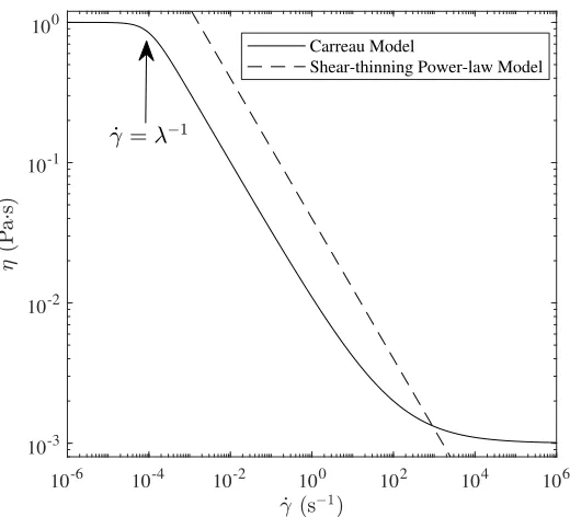
bot-tom edge held stationary. The material will experience a strainγ =dl/l. . . 2 1.2 Comparison of the viscosity vs. shear rate predicted by the Carreau model and
the power-law model. For both models,n = 0.5, while for the Carreau model,
η∞ =10−3 Pa·s,η0= 1 Pa·s,λ=10−4s. . . 6
1.3 Graphical schematic of the Maxwell model of a viscoelastic fluid, consisting
of a viscous dashpot and an elastic spring connected in series.λM = η/Gis the characteristic relaxation time of the model. . . 7
1.4 G0andG00vs. ωfor the Maxwell model withλ
M =0.1 s andη=105Pa·s. The crossover frequencyω =λ−1
M is indicated with an arrow. . . 10
1.5 Common geometries used for shear rheometry. (a) Cone-and-Plate, (b) Parallel
Plate, and (c) the Couette, or concentric cylinder, geometry. [2] . . . 11
2.1 (a) The simulation geometry. Fluid space is coloured blue. The tungsten wire is
shaded gray. (b) The simulation mesh. (c) A magnified view of the mesh near
the wire. The region shown in (c) is approximately square, with side length 16Rw. 21
2.2 Plots of viscosity vs. shear rate for the Carreau model withη0 = 1 Pa·sη∞ = 10−3Pa·s, and several different values ofλandn. . . . 26
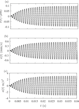
2.3 The x-components of the (a) position, (b) velocity, and (c) acceleration of the
center of the wire as a function of time for a simulation of a wire vibrating in a
Newtonian fluid withη=3×10⁻³Pa·s and f =900 Hz. The lines connect the data points to aid the eye. Note the difference in units between the plots. The simulation time extends to 0.089 s, but only the first 0.04 s are plotted here to
emphasize the early-time transient. . . 29
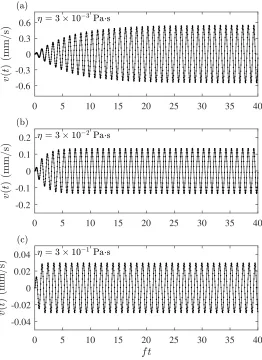
2.4 The velocity in the x direction of the center of the wire vs. normalized time
f tfor simulations of a wire vibrating in a Newtonian fluid at a frequency near
the resonance frequency with a) ηsim = 3× 10⁻³, b) ηsim = 3×10⁻², and c)
ηsim = 3 × 10⁻¹ Pa·s. The early-time transient damps out faster for higher viscosities. . . 31
2.5 Example fit of Eq. 2.22 (red curve) to the late-time velocity data from Fig. 2.3
(b). . . 32
2.6 The velocity resonance curves for the Newtonian-fluid simulations with
vis-cosities shown in the legend. The inset is a magnified view of the
smaller-amplitude resonance curves obtained at higher viscosities. The lines connect
the data points to aid the eye. . . 32
2.7 (a) The resonant frequency fr, (b) the full width at half maximum∆f, and (c) the quality factor Q vs. ηfor simulations of a wire vibrating in a Newtonian
fluid. The curves in each plot are theoretical predictions calculated using Eq. 2.1. 33
2.8 (a) Real and imaginary components, and (b) magnitude and phase of the
sim-ulated velocity of a wire vibrating in a Newtonian fluid with η = 10−2 Pa·s plotted vs. frequency. The lines are fits of Eq. 2.1 to the data. . . 33
2.9 (a)ηf itvs.ηsimfrom fits of the real component of Eq. 2.1 to the real component
of the resonance curves for simulations of a wire vibrating in a Newtonian fluid.
(b) The magnitude of the % difference betweenηf itandηsimvs.ηsim. . . 34
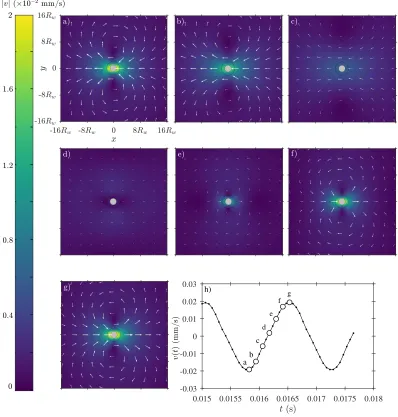
2.10 Snapshots from a simulation of a wire vibrating in the xdirection in a
shear-thinning fluid described by Eq. 2.10 withn= 0.5 andλ= 102s. The wire was driven at f =680 Hz, which was close to its resonant frequency. (a) - (g) show the spatial variation of the velocity of the fluid near the wire at times covering
a half-period of the wire’s oscillation. The magnitude of the velocity is given
by the surface plot, while the arrows show velocity direction and logarithmic
magnitude. (h)v(t), the velocity of the vibrating wire. The labelled time points
in (h) indicate the times of the corresponding velocity plots. The coordinate
system is explicitly labelled in subplot (a). A video showing the full domain
and all times for this simulation is included in the supplementary media. . . 36
2.11 Snapshots from a simulation of a wire vibrating in the xdirection in a
shear-thinning fluid described by Eq. 2.10 with n = 0.5 and λ = 102 s. The wire
was driven at f = 680 Hz, which was close to its resonant frequency. (a) -(g) show the spatial variation of the shear rate near the wire at times covering
a half-period of the wire’s oscillation. (h) v(t), the velocity of the vibrating
wire. (i) ˙γr¯(t), the shear rate averaged around the circumference of the wire,
as described in the text. The labelled time points in (h) and (i) indicate the
times of the corresponding shear rate plots. The coordinate system is explicitly
labelled in subplot (a). A video showing the full domain and all times for this
simulation is included in the supplementary media. . . 37
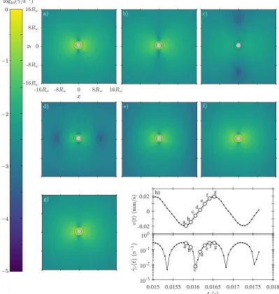
2.12 Snapshots from a simulation of a wire vibrating in the xdirection in a
shear-thinning fluid described by Eq. 2.10 with n = 0.5 and λ = 102 s. The wire was driven at f = 680 Hz, which was close to its resonant frequency. (a) - (g) show the spatial variation of the viscosity near the wire at times covering a
half-period of the wire’s oscillation. (h)v(t), the velocity of the vibrating wire. (i)
η¯r(t), the viscosity averaged around the circumference of the wire, as described
in the text. The labelled time points in (h) and (i) indicate the times of the
corresponding viscosity plots. The coordinate system is explicitly labelled in
subplot (a). A video showing the full domain and all times for this simulation
is included in the supplementary media. . . 38
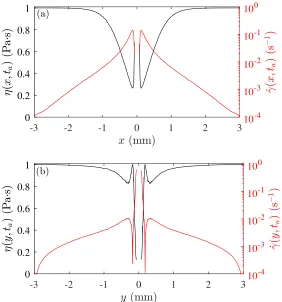
2.13 Fluid viscosity and shear rate as a function of (a) x, along the liney = 0, and (b)y, along the linex = 0, at the time of Fig. 2.12 (a). The gap in the data in the center of each plot corresponds to the location of the wire. . . 40
2.14 The velocity in the xdirection of the center of the wire vs. normalized time f t
for simulations of a wire vibrating in a shear-thinning fluid described by the
Carreau model (Eq. 2.10) with (a)n = 0.7, λ= 103 s, (b)n = 0.5, λ= 103 s, (c)n = 0.7,λ= 104 s, and (d)n= 0.5,λ= 104s. Note that for the simulation in subplot (d), the simulation time extends to f t = 40, but only the first 20 oscillations are plotted here to emphasize the early-time transient. . . 41
2.15 Velocity resonance curves (black curves) and the spatiotemporal average
vis-cosity ¯η(f) (gray curves), for the full parameter space covered by our
shear-thinning simulations. Note the difference in velocity scale between subplots. . . 42 2.16 ¯η(fr) plotted against 1/λ for simulations of a wire vibrating in shear-thinning
fluids. . . 43
2.17 (a) The resonant frequency fr, (b) the full width at half maximum∆f, and (c) the quality factorQplotted against 1/λ for the simulations of a wire vibrating
in shear-thinning fluids. . . 44
2.18 (a) The resonant frequency fr, (b) the full width at half maximum∆f, and (c) the quality factorQfor the simulations of a wire vibrating in shear-thinning
flu-ids plotted against ¯η(fr) and compared to the theoretical predictions calculated
from Eq. 2.1 (black curves). . . 44
2.19 (a) Real and imaginary components, and (b) the magnitude and phase of the
of the velocity vs. frequency with fits of Eq. 2.1 to each component for the
simulation of a wire vibrating in a shear-thinning fluid withn=0.5 andλ=103s. 45
2.20 (a) ηf it vs. ¯η(fr) for the simulations of a wire vibrating in shear-thinning
flu-ids. Results with the same nare plotted with the same colour, and the same
λare plotted with the same symbol. (b) The magnitude of the % difference between the two viscosities vs. ¯η(fr). The error bars are the standard deviation
between theηf it values determined by independent fits of the components of
the resonance curves to Eq. 2.1. . . 45
3.1 Photographs of the vibrating-wire rheomter (left) and the temperature-controlled
housing and magnets (center), and a schematic diagram of the instrument as
seen looking through the face of the magnet (right). Colour online. . . 57
3.2 A schematic diagram of the experimental setup. . . 59
3.3 Voltage induced in the vibrating wire as a function of frequency for ethanol at
9.7◦C. The curves are independent fits the real and imaginary parts of Eq. 3.1
to each component. . . 62
3.4 The viscosity determined from fits to vibrating-wire data as in Fig. 3.3, ηf,
plotted against expected viscosity,ηe. The solid line isηf =ηe. The fluids were ethanol and silicone oil at temperatures ranging from 5 to 60◦C.
Uncertain-ties in the measured viscosiUncertain-ties are smaller than the size of the symbol. Inset:
Difference between the measured and expected values. . . 63
3.5 In-phase and out-of-phase components of the measured voltage for a 3.5 wt%
aqueous solution of HEC. The black lines are independent fits of the real and
imaginary parts of Eq. 3.1 to the components with the complex viscosity
sub-stitution, Eq. 3.8. Only every 10th data point is plotted for clarity. . . 64
3.6 Viscoelastic moduli for a 3.5 wt% solution of HEC in water. The data spanning
1−100 Hz (open symbols) were obtained from a shear rheometer using
time-temperature superposition. The data at approximately 1000 Hz (solid symbols)
were obtained with vibrating-wire rheometers with lengthsL= 5 and 6 cm, as described in the text. . . 64
3.7 Viscoelastic moduli of a 1 wt% Laponite suspension vs. frequency after
ap-proximately 4 h of aging. Data in (a) were measured using a shear rheometer.
Data in (b) were determined from dynamic light scattering (open symbols) and
with the vibrating-wire rheometer (solid symbols). . . 66
3.8 The in-phase component of the voltage measured with the vibrating-wire
rheome-ter for an aging Laponite clay suspension. From largest to smallest amplitude,
the curves correspond to aging times of 40 min, 22 h, 52 h, and 144 h. . . 67
3.9 Viscoelastic moduli of the 1% Laponite suspension measured with the
vibrating-wire rheometer plotted as a function of aging time. Error bars are not shown
for clarity, but are similar to those plotted in Fig. 3.6. . . 67
4.1 G0 (filled symbols) andG00 (open symbols) vs. strain amplitudeγ at an
angu-lar frequencyω = 1 rad/s for the 18 wt. % Pluronic solution at temperatures that increase counter-clockwise fromT = 10◦ C in (a), to T = 85 ◦C in (f). The data are at temperatures in: (a) the temperature sol state, (b) the
low-temperature sol-gel transition, (c) the gel state, a few degrees warmer than the
sol-gel transition, (d) the gel state, a few degrees cooler than the gel-sol
tran-sition (e) the high-temperature gel-sol trantran-sition, and (f) the high-temperature
sol state. Data in rheologically similar states share the same row. . . 79
4.2 G0(filled symbols) andG00 (open symbols) vs. angular frequencyωat a strain
amplitude γ = 0.2% for the 18 wt. % Pluronic solution at temperatures that increase counter-clockwise from T = 10 ◦ C in (a), to T = 85 ◦C in (f). The data are at temperatures in: (a) the temperature sol state, (b) the
low-temperature sol-gel transition, (c) the gel state, a few degrees warmer than the
sol-gel transition, (d) the gel state, a few degrees cooler than the gel-sol
tran-sition (e) the high-temperature gel-sol trantran-sition, and (f) the high-temperature
sol state. Data in rheologically similar states share the same row. . . 80
4.3 G0 (black) andG00 (gray) measured at ω = 1 rad/s andγ = 1% for aqueous solutions of Pluronic with concentrations 16 wt. % (left), 18 wt. % (center) and
20 wt. % (right) while heating (top) and cooling (bottom) at a rate of 6◦C per
hour. . . 82
4.4 (a)G0(t) (black) andG00(t) (gray) measured atω = 1 rad/s andγ = 1% during an experiment in which the temperature of the 18 wt. % solution was changed
in discrete steps. (b) The temperature as a function of time. The steps indicated
by the arrows in (a) correspond to the relaxation curves shown in Fig. 4.7. . . . 84
4.5 G0(t) (black) andG00(t) (gray) measured at ω = 1 rad/s and γ = 1% in the high temperature regime of the discrete temperature study of the (a) 18 wt. %
and (b) 20 wt. % solutions. The temperature profile is the red step-like curve
(see color figure online) using the right axis. The vertical arrow indicates the
change in behaviour discussed in the text. The transition temperaturesT2 and
T3 determined from the continuous heating and cooling ramp experiments are
shown with the labelled arrows. . . 85
4.6 Temperature-concentration phase diagram for aqueous solutions of Pluronic
F127. The results of the present work are displayed as the hatched bars, as
described in the legend. For a given concentration, the left half of the bar shows
the states observed when heating, while the right half shows the states observed
when cooling. The width of the bars has no physical significance. Results from
previous work are shown by the symbols, with corresponding references given
in the legend. . . 87
4.7 Relaxation of the moduli of the 18 wt. % Pluronic solution following a step
change in temperature. The four subplots correspond to the steps labeled in
Fig. 4.4. The red dashed lines (see color figure online) are independent fits
toG0(t) andG00(t). a) T = 24.4 ◦C (warming), b)
T = 66 ◦C (warming), c)
T =76◦C (cooling), and d)T = 25◦C (cooling). . . 90 4.8 Slow and fast relaxation times,τs, andτf respectively, determined by fittingG0
andG00 to Eq. 4.1 following a step inT while heating and cooling. Gray
sym-bols indicate relaxation times that are less reliable, as described in the text. The
shaded regions show the temperature range over which the transitions occur, as
determined from the continuous temperature ramp experiments. . . 91
A.1 The temperature measured in the fluid circulating around the vibrating wire vs.
time. . . 107
A.2 Fits of Eq. A.1 (red curves) to the real component of the measured voltage from
the wire vibrating in water at (a)T = 15, (b) 50, and (c) 75◦C. . . 107 A.3 The measured resonant frequency fr and the resonant frequency predicted by
Eq. A.1 (red curve) vs. T when (a) heating, and (b) cooling. The theoretical
predictions assume that only the fluid density and viscosity change with
tem-perature. . . 108
A.4 The viscosity of water (black dots) determined from fits of the real component
of Eq. A.1 to the real component of the measured voltage and the temperature
in the circulating fluid around the vibrating wire (red dots) vs. time. . . 109
A.5 The mean of 5 measurements of ηf it near the end of the 30 min waiting time
at each temperature plotted against T when (a) heating and (b) cooling. The
standard deviations are smaller than the symbols in all cases. The red curves
are the expected viscosity determined from the NIST Chemistry Webbook. (c)
The percentage difference between the mean values of ηf it and the expected viscosity when heating, and (d) when cooling. For the most part, the standard
deviation of the percentage difference is smaller than the symbols. . . 110 A.6 Surface plots showing (a) the resonant frequency fr, (b) the full width at half
maximum∆f, and (c) the quality factorQvs.G0andG00. . . 111 B.1 Fits of the real and imaginary components of Eq. A.1 (black curves) to the real
and imaginary components of the measured voltage of the 6 cm wire vibrating
in the 18 wt.% Pluronic solution at (a)T = 20◦C and (b)T =35◦C. (c) and (d) show the differenceδV between the data and the fit at the same temperatures as (a) and (b), respectively. The imaginary component of the measured voltage,
fit, and the resultingδVhave been artificially shifted to lower voltage for clarity.
Note that in subplot (d) only the data for f <3000 Hz are shown to emphasize
the low-frequency peaks. . . 113
B.2 Surface plots showing χ2 vs.G0
andG00 from the restricted fitting routine
de-scribed in the text of the imaginary component of Eq. A.1 to the imaginary
component of the measured voltage of the 6 cm wire vibrating in the 18 wt.%
Pluronic solution at temperatures spanning 15 to 85◦C, as labeled in the figure.
The global minimum in each plot is marked with a red circle. . . 116
B.3 G0wire andG00wire (symbols), measured using the vibrating wire as described in
the text, and G0shear and G00shear (curves), measured using the shear rheometer
as described in Chap 4, for aqueous solutions of Pluronic with concentrations
14, 16, 18, and 20 wt.%, increasing from left to right, while heating (top) and
cooling (bottom). . . 117
B.4 G0 andG00 vs. ω measured using the shear rheometer (data atω < 103 rad/s)
as described in Chap. 4, and the vibrating-wire rheometer (data at ω > 103
rad/s) at temperaturesT =(a) 10, (b) 35, (c) 55, and (d) 85◦C. The error bars plotted for the high-frequency vibrating-wire data show the full width at half
maximum of the resonance curves. Except in Fig. B.4 (a), the error bars are
smaller than the data symbols. The dashed lines in (a) and (d) showG00 ∼ ω1. . 118
List of Tables
2.1 Details of the simulation meshes. Symbols are defined in the text. . . 23
4.1 a) TemperaturesTiat the start of a phase transition and the corresponding width
of the transition∆Timeasured from the continuous heating and cooling ramps shown in Fig. 4.3. The uncertainties inTiand∆Tiare approximately±0.01◦C. b) TemperaturesTi at which the the rheological relaxation time becomes long,
and the corresponding range of temperatures over which long relaxation times
∆Ti are observed, obtained from the temperature-step experiments shown in Figs 4.4-4.8. The uncertainties in the last digit of the entries in part (b) are
given in parentheses and depend on the step size used in the experiment, as
discussed in Sec. 4.3.3. . . 84
List of Symbols
τ Shear stress
F Force
A Area
γ Shear strain
l Deformation length
G,G0 Elastic modulus
G00 Viscous modulus
˙
γ Shear rate
η Dynamic viscosity
K Fluid consistency index
n Power-law index
η∞ Viscosity at infinite shear rate
η0 Viscosity at zero shear rate
λ Relaxation time
τy Yield stress
ω Angular frequency
f Frequency
t Time
M Torque
R Cylinder radius
L Length
θ Angular displacement
V Voltage
Λ Voltage amplitude
f0 Resonant frequency of a vibrating wire in vacuum
∆0 Self-damping of a vibrating wire
β Added mass
β0 Viscous damping
ρ Density
m Mass
g Gravitational acceleration
v Velocity
e Size of computational mesh element
Ne Number of mesh elements
ρe Density of mesh elements
A Arbitrary vector
A Arbitrary tensor
p Pressure
τf Fast relaxation time
τs Slow relaxation time
List of Abbreviations
HEC 2-hydroxyethyl cellulose
PPO Poly(propylene oxide)
PEO Poly(ethylene oxide)
DLS Dynamic light scattering
SAXS Small angle X-ray scattering
SANS Small angle neutron scattering
Chapter 1
Introduction
Rheology is the study of how materials flow or deform. Materials of interest to rheology
range from simple Newtonian fluids like water or vegetable oil, to viscoelastic polymeric
ma-terials like plastics used in injection moulding, to asphalt used to pave our streets. Even the
mantle of our planet can be described as a viscoelastic material [1]. Studying how materials
behave when deformed is essential for fundamentally understanding what they are made of and
how to manipulate their properties for industrial and commercial use. In this chapter we will
build up the physical framework used in studying the rheological behaviour of materials.
1.1
Fluids
A diagram depicting the deformation of a two-dimensional cross-section of a region of
material is shown in Fig. 1.1 [2]. With the bottom edge held stationary, the material will
deform in response to an applied shear stress
τ= F
A, (1.1)
Chapter1. Introduction 2
whereF is the applied shearing force andAis the surface area. The deformation, or the shear
strain, is
γ= dl
l , (1.2)
wherelis the height of the fluid region anddlis the deformation length. For small shear strains,
γ is approximately the angle shown in the figure. For ideal elastic materials, the constitutive
Figure 1.1: A cross-section segment of a material subject to a shear stress τ, with the bottom edge held stationary. The material will experience a strainγ= dl/l.
relationship, i.e., the relationship between stress and strain, is given by
τ=Gγ, (1.3)
whereGis the elastic modulus. As long as the applied shear stress (or shear strain) is small,
the material will return to its original position when the applied stress is removed. This is the
2-dimensional form of Hooke’s law. For large strains, irreversible deformation like stretching
or fracture may occur, in which case Eq. 1.3 no longer applies and the relationship between
stress and strain is nonlinear.
For Newtonian fluids, the shear stress is related to the rate of deformation, i.e., the shear
rate
˙
γ= dγ
Chapter1. Introduction 3
through Newton’s law of viscosity
τ=ηγ,˙ (1.5)
whereηis the dynamic (shear) viscosity. Even for a very small stress, a Newtonian fluid will
deform irreversibly, i.e., it will flow.
The discussion above is a simple two-dimensional view of stresses and strains. In general,
constitutive relationships are three-dimensional and stress, strain and related quantities are
de-scribed by tensors [3]. A complete discussion of tensorial constitutive relationships is beyond
the scope of this work, and we will restrict our discussion to simple two-dimensional models.
The constitutive relationships described above apply only to a small subset of materials.
Solid materials such as ceramics and metals will obey Hooke’s law for small strains, but
frac-ture when the strain is too large [3]. Many simple fluids such as water, honey, or vegetable
oil obey Newton’s law of viscosity [4]. There are, however, many materials, called complex
fluids, that behave somewhere between ideal viscous or ideal elastic materials, i.e., they are
viscoelastic. We will begin our discussion of complex fluids by discussing non-Newtonian
viscous behaviour.
1.1.1
Shear Thinning and Shear Thickening
For Newtonian fluids at constant temperature and pressure, viscosity is independent of
shear stress or shear rate. For many fluids this is not the case, and viscosity depends on the
shear rate. A simple constitutive model that illustrates this non-Newtonian behaviour is the
power-law model:
τ= Kγ˙n, (1.6)
whereKis the fluid consistency index andnis the law index. The viscosity of a
power-law fluid is the ratio of the shear stress to the shear rate:
Chapter1. Introduction 4
Forn = 1 the fluid is Newtonian; the viscosity is independent of shear rate. For 0< n <1 the fluid is shear-thinning, i.e., the viscosity decreases with increasing shear rate. Many polymeric
solutions and particle dispersions exhibit shear-thinning behaviour[3]. A few examples are
blood, ketchup, and paint. Blood, a complex fluid consisting of different types of cells in solu-tion, forms aggregates of red blood cells when at rest [5]. These aggregates give blood a rigid
structure that must be broken apart before the material will flow, i.e., the material possesses a
yield stress, as discussed below. Break-up of the aggregates when the blood is sheared results
in shear-thinning [5, 6]. Ketchup is a complex suspension of tomato matter, i.e., cell wall
frag-ments and cellular material in a mixture of water, vinegar, and other additives. The suspended
cellular particles aggregate when at rest, forming a rigid structure that gives ketchup a yield
stress [7]. Shear-thinning arises then from the break-up of that structure when the ketchup
sheared. The previous two fluids are examples of colloidal suspensions. Colloidal suspensions
may also exhibit shear-thickening, as discussed below. Shear-thinning is also found in polymer
solutions. In dilute polymer solutions, shear-thinning is due to a reduction in the drag on a
polymer chain when it is stretched in the flow direction [3]. Ultimately the mechanism behind
shear-thinning is the rearrangement of micro-structure in the fluid when it is sheared.
If n > 1 in Eq. 1.7, viscosity increases with increasing shear rate; the fluid is
shear-thickening. Shear-thickening is found most prevalently in concentrated dispersions of
par-ticles, although some polymer systems have been observed to shear thicken under specific
conditions [8]. One example of a shear-thickening dispersion is cornstarch in water. At the
microscopic scale, cornstarch is irregularly shaped particles with a diameter of approximately
5−20 µm [9]. Shear-thickening in cornstarch dispersions arises from the jamming together
of cornstarch particles in response to an applied force, giving them the ability to resist motion
and dissipating energy. This mechanism is common among all shear-thickening dispersions of
particles [8]. Shear-thickening fluids can be exploited in a number of different ways, such as in liquid body armour when integrated with ballistic fabric [10], and shock absorption when
Chapter1. Introduction 5
The power-law model given by Eq. 1.7 is unphysical for many fluids in both the high and
low shear-rate limits. In the shear-thinning case, it suggests that as ˙γ → 0, η → ∞, and as
˙
γ → ∞,η → 0. Although for yield-stress fluids, which will be discussed below, the viscosity
is infinite at zero shear rate, it approaches a constant value at high shear rates. In addition,
for shear-thinning polymer solutions, at very low and very high shear rates the viscosity is
constant [3].
An alternative model that incorporates the plateau viscosities at high and low shear rates is
the Carreau model,
η=η∞+(η0−η∞)
h
1+(λγ˙)2i(n−1)/2, (1.8) whereη∞ is the viscosity at infinite shear rate, η0 is the viscosity at zero shear rate, and λis
the relaxation time [4]. The relaxation time determines the location of the crossover between
the low shear-rate Newtonian plateau and the intermediate shear-rate power-law behaviour, as
shown in Fig. 1.2. The Carreau model and the power-law model are compared in Fig. 1.2. For
both models shown, the shear-thinning index isn= 0.5. The Carreau model exhibits power-law shear-thinning behaviour over a limited range of shear rate.
1.1.2
Yield Stress
Some materials cannot flow unless the applied stress exceeds a critical value known as
the yield stress. At an applied stress greater than the yield stress, the material behaves like a
viscoelastic liquid and will flow. Below the yield stress the material behaves like an elastic
solid. The simplest model of a yield stress fluid is the Bingham model [12]. For an applied
stress that exceeds the yield stress,
τ=τy+ηpγ,˙ (1.9)
whereτy is the yield stress andηpis the infinite shear-rate ‘plastic’ viscosity. Once yielded, the
Bingham model describes a fluid with a viscosity that shear-thins and approaches ηp at high
Chapter1. Introduction 6
10-6 10-4 10-2 100 102 104 106 10-3
10-2 10-1 100
Carreau Model
Shear-thinning Power-law Model
Figure 1.2: Comparison of the viscosity vs. shear rate predicted by the Carreau model and the power-law model. For both models, n = 0.5, while for the Carreau model,η∞ = 10−3 Pa·s, η0 =1 Pa·s,λ=10−4s.
The next simplest model is the Herschel-Bulkley model [13], which describes a yield-stress
fluid that allows for a nonlinear increase of stress with shear rate. For this model, again, when
the applied stress is less than the yield stress the fluid does not flow ( ˙γ = 0). For an applied stress greater than the yield stress,
τ=τy +kγ˙n, (1.10)
where k is the fluid consistency index, similar to the power-law model. Indeed, the second
term in this constitutive model is simply the power-law model. In many cases, the behaviour of
real yield-stress fluids is better described by the Hershel-Bulkley model then by the Bingham
model.
Yield stress fluids are very common in our day-to-day life. They are often found in our
bathroom cabinets — shaving gel, toothpaste, or cosmetic creams — or in our refrigerators
— mayonnaise, whipped cream, or ketchup. Tooth paste will flow out of the tube when you
Sim-Chapter1. Introduction 7
ilarly, mayonnaise will flow when you spread it on a sandwich, but it retains its shape in its
container, even if it is tilted. An understanding of what causes the yield stress, and how to
tune it, is important from a practical perspective when designing consumer products. Yield
stress fluids are also prevalent in industry. One example arises in the transport of waxy crude
oil through pipelines. Waxy crude oil exhibits a yield stress [14], and understanding how the
yield stress influences pressudriven flow in a pipe is of importance to oil transport and
re-covery [15].
1.1.3
Viscoelasticity
The discussion so far has been about how the steady-shear viscosity of non-Newtonian
flu-ids can differ from that of Newtonian fluids. We have mentioned that non-Newtonian flow be-haviour arises from the presence of structure within the fluid. This structure may also contribute
elasticity to the fluid. Materials that exhibit both viscous and elastic-like behaviour are called
viscoelastic. One of the simplest models of a viscoelastic fluid is the Maxwell model. This
Figure 1.3: Graphical schematic of the Maxwell model of a viscoelastic fluid, consisting of a viscous dashpot and an elastic spring connected in series. λM = η/G is the characteristic relaxation time of the model.
model was erroneously [3] proposed by James Clerk Maxwell in 1867 to describe gases [16],
but it has since been adopted in rheology to describe simple viscoelastic fluids. The Maxwell
model incorporates viscous and elastic behaviour into one constitutive equation. The model
can be graphically represented by a viscous dashpot and an elastic spring connected in series
as shown in Fig. 1.3. The stress-strain relationships for the individual elements have already
been introduced in Eqs. 1.3 and 1.5. When subject to a stress, the total strain in a Maxwell
Chapter1. Introduction 8
springγE, i.e.,γ = γD+γE. The stress acting on each element is the same, i.e.,τ = τD = τE. To obtain a relationship between stress and shear rate we differentiate both sides of the strain relation with respect to time
˙
γ=γ˙D+γ˙E. (1.11)
The shear rate from the dash-pot is related to stress through Eq. 1.5, while the shear rate from
the elastic spring can be calculated from the time-derivative of Eq. 1.3, yielding
˙
γ = τη+ 1
G dτ
dt (1.12)
or, after rearranging and defining the relaxation timeλM =η/G,
τ+λM
dτ
dt =GλMγ.˙ (1.13)
This model describes a material with only one relaxation time. Real materials typically have
more than one relaxation time [4]. To account for this, many Maxwell elements can be
com-bined in parallel into the Generalized Maxwell Model [4], where Eq. 1.13 represents the stress
and strain in one element, and the total stress in the material is the sum of the stresses in all of
the elements.
1.1.4
Small-Amplitude Oscillatory Shear
A common experimental method for studying viscoelastic materials is to apply an
oscil-latory shear strain (or stress) and measure the resulting stress (or strain). For this discussion
we will consider an applied strain. We assume here that the amplitude of the applied strain is
sufficiently small that the response of the material is linear. We consider an oscillatory shear strain of the form
Chapter1. Introduction 9
whereγ0 is the strain amplitude andω is the angular frequency. If this strain is applied to an
elastic material that obeys Hooke’s law (Eq. 1.3), the resulting stress is
τ(t)=Gγ0sin(ωt), (1.15)
i.e., the stress is sinusoidal and in phase with the applied strain. If the strain is applied to a
viscous fluid that obeys Newton’s Law of Viscosity (Eq. 1.5), the resulting stress is
τ(t)=ηωγ0cos(ωt), (1.16)
i.e., the stress is sinusoidal and 90◦ out of phase with the applied strain. In general, for a
viscoelastic fluid, the phase difference φ between the applied strain and resulting stress will be somewhere between 0 and 90◦ [17], i.e., τ(
t) = τ0sin(ωt+φ). This can be expanded into
in-phase and out-of-phase components:
τ(t)=τ0cos(φ) sin(ωt)+sin(φ) cos(ωt). (1.17)
The amplitude of the in-phase and out-of-phase components divided by the strain amplitude are
known as the elastic modulusG0(ω) and the viscous modulusG00(ω), respectively. In general,
the moduli depend on frequency. Eq. 1.17 can therefore be written as
τ(t)
γ0
=G0(ω) sin(ωt)+G00(ω) cos(ωt). (1.18) Comparing this form to Eqs. 1.15 and 1.16, we can identify the viscoelastic moduli for elastic
solids and Newtonian liquids as
G0(ω)=G (1.19)
Chapter1. Introduction 10
for an elastic solid, and
G0(ω)= 0 (1.21)
G00(ω)= ηω (1.22)
for a Newtonian liquid. For viscoelastic fluids, the dependence of the moduli on frequency is
10-2 100 102 104 106
10-2 100 102 104 106
Figure 1.4: G0 andG00 vs. ω for the Maxwell model withλM = 0.1 s andη = 105 Pa·s. The crossover frequencyω=λ−1
M is indicated with an arrow.
more complicated. For the Maxwell model presented above, the viscoelastic moduli are [4]
G0(ω)= ηλMω
2
1+λ2
Mω2
, (1.23)
G00(ω)= ηω 1+λ2
Mω2
. (1.24)
Chapter1. Introduction 11
1.1.5
Shear Rheometry
One of the more common experimental tools used in rheology is the shear rheometer. Shear
rheometers work by confining a fluid within a geometry, applying a strain, and measuring the
stress (or applying a stress and measuring the strain). Three common geometries used for shear
rheometry are shown in Fig. 1.5. For all three of the geometries shown, one component of the
geometry is typically held fixed, e.g., the bottom plate in the Cone-and-Plate or Parallel Plate
geometries is held fixed while the top plate is rotated. Most of the shear rheometry done in
this thesis used the Couette cell geometry, with the outer cylinder held fixed while the inner
cylinder was rotated.
Figure 1.5: Common geometries used for shear rheometry. (a) Cone-and-Plate, (b) Parallel Plate, and (c) the Couette, or concentric cylinder, geometry. [2]
The rheometer used in this thesis was an Anton-Paar MCR-302 shear rheometer. The
rhe-ological parameters extracted from an experiment are the shear stress and shear strain, which
are then related to material properties such as the viscous and elastic moduli as outlined in
the previous section. Rheometers do not directly measure these quantities, however. Instead,
they measure the torque M on the tool and the angular displacementθof the tool, then relate
these quantities to the shear stress and shear strain, respectively. The relations between these
quantities depend on the geometry being used. For an ideal Couette cell in the small gap limit,
the stress is related to the torque through [3]
τ= M
2πR2
iL
Chapter1. Introduction 12
whereRi is the radius of the inner cylinder andLis its length. The shear strain is related to the
angular displacement by
γ =θ Ro+Ri
2(Ro−Ri)
, (1.26)
whereRois the radius of the outer cylinder.
There are a few experimental limitations that restrict the range of moduli and frequencies
that a shear rheometer can probe [18]. Rheometers have both high and low frequency limits.
The low frequency limit is more a limit of practicality, as the measurement time per point at
low frequency gets very long. Most shear rheometers, including the one used in this thesis,
are restricted to frequencies less than 100 Hz [19]. In addition, the inertia of the instrument
and the sample limit the high-frequency operation of the rheometer, causing the instrument to
report a quadratic increase in the moduli with frequency at high frequencies [18]. In addition,
the capabilities of the instrument put a limit on the smallest and largest torques that can be
measured. For the MCR-302 rheometer used in this work, the minimum measurable torque
is 0.01 µN·m and the maximum measurable torque is 200 mN·m [19]. This sets upper and
lower limits on the magnitude of the moduli the rheometer can measure. The lower limit also
helps motivate the development of the vibrating-wire rheometer discussed in Chap. 2, since it
prevents the study of low-viscosity fluids with shear rheometers.
1.2
Summary of Present Work
1.2.1
Overview
The majority of the work presented in this thesis focusses on the development of a novel
rheometer based on a vibrating wire that allows for the measurement of viscoelastic moduli
at high frequencies and low viscosities, both regimes which are inaccessible to conventional
shear rheometers. This was investigated both experimentally through the construction and
Chapter1. Introduction 13
in Newtonian and shear-thinning fluids using COMSOL Multiphysics.
1.2.2
Numerical Simulations of the Forced Oscillations of a Wire in a
Fluid
In Chap. 2 we use COMSOL Multiphysics software to numerically study the two-dimensional
forced oscillations of a wire vibrating in Newtonian fluids and shear-thinning fluids described
by the Carreau model. When the wire is subject to a sinusoidal driving force, it exhibits
reso-nant behaviour that depends on the viscosity of the fluid it is in. The simulations of the wire
vibrating in a Newtonian fluid were extremely well described by the theory for a wire vibrating
in a Newtonian fluid developed by Retsinaet al.[20, 21]. Our simulations of a wire vibrating
in a Carreau fluid revealed resonant behaviour similar to the behaviour of the wire vibrating
in Newtonian fluids. We find that the shear rate and viscosity in the fluid vary significantly in
both space and time. The theory of a wire vibrating in a Newtonian fluid could describe the
behaviour of a wire vibrating in a Carreau fluid if the viscosity in the theory is set equal to
the viscosity averaged spatially around the circumference of the wire and over one period of
oscillation.
1.2.3
Vibrating-wire Rheometry
In Chap. 3 we describe the design and operation of a novel vibrating-wire rheometer. Our
device consists of a tungsten wire under tension and immersed in a fluid in a magnetic field.
When an alternating current is passed through the wire it vibrates at the driving frequency,
and we measure the voltage induced across the wire as a function of frequency. The resonant
frequency of the wire is of order 1000 Hz, and can be tuned by varying its length and the
applied tension. We modify an analytic expression for the induced voltage, previously derived
for Newtonian fluids, to include a complex viscosity, and determine the viscous and elastic
Chapter1. Introduction 14
results for the viscosity of Newtonian fluids and the viscoelastic moduli of aqueous polymer
solutions, at frequencies higher than those accessible using a conventional shear rheometer.
Because the amplitude of the wire’s vibrations is on the order of a few microns, it can be used
to probe the microrheology of fluids that are heterogeneous on that scale. We illustrate this by
measuring the micron-scale moduli of a viscoplastic suspension of Laponite clay as it gels.
1.2.4
Gelation Dynamics of Aqueous Solutions of Pluronic F127
In Chap. 4 we study the gelation dynamics of solutions of Pluronic F127, a triblock
copoly-mer, using oscillatory rheometry. As a sufficiently concentrated solution is slowly and contin-uously heated from 10 to 85◦C, it undergoes a transition from sol to gel around room
tempera-ture, followed by a gel-sol transition at a higher temperature. The sol-gel transition temperature
decreases and the width in temperature of the gel phase broadens with increasing
concentra-tion. The transitions occur over a temperature range of a few degrees, over which the viscous
and elastic moduli change by more than 5 orders of magnitude. On cooling, the width in
tem-perature of the gel phase is larger and the transitions themselves extend over a larger range of
temperature. Near the phase transitions, the rheological relaxation time becomes very long —
up to of order 104s. Gelation in Pluronic solutions is due to the arrangement of micelles into
clusters that grow in size to form a large-scale lattice, and our results indicate that changes in
microstructure that accompany the equilibration of these clusters happen very slowly.
1.2.5
Appendices
In App. A we present additional measurements using our vibrating-wire rheometer. We
study the influence of temperature on the resonant frequency of the wire and the measured
vis-cosity in water. We find that although the resonant frequency of the wire changes significantly
with temperature, by allowing it to be a free parameter in our curve fitting routine, the viscosity
of water can still be accurately determined. In addition, we investigate how the shape of the
Chapter1. Introduction 15
In App. B we present measurements of the viscoelastic properties of aqueous solutions of
Pluronic made using our vibrating-wire rheometer. Allowing for the difference in frequency, our results are fully consistent with measurements of the viscoelastic properties of Pluronic
using a shear rheometer presented in Chap. 4.
Bibliography
[1] W. R. Peltier. Mantle Convection and Viscoelasticity. Annu. Rev. Fluid Mech., 17:561–
608, 1985.
[2] J. R. de Bruyn and F. K. Oppong. Rheological and microrheological measurements of
soft condensed matter. In J. Olafsen, editor,Experimental and Computational Techniques
in Soft Condensed Matter Physics. Cambridge University Press, 2010.
[3] Christopher W. Macosko.Rheology: Principles, Measurements, and Applications.
Wiley-VCH, 1994.
[4] F. A. Morrison. Understanding Rheology. Oxford University Press, 2001.
[5] J. Goldstone, H. Schmid-Schonbein, and R. Wells. The rheology of red blood cell
aggre-gates. Microvasc. Res., 2:273–286, 1970.
[6] E. W. Merrill. Rheology of blood. Physiol. Rev., 49, 1969.
[7] E. Bayod, W. P. Willers, and E. Tornberg. Rheological and structural characterization
of tomato paste and its influence on the quality of ketchup. LWT Food Sci. Technol.,
41:1289–1300, 2008.
[8] J. Ding, P. J. Tracey, W. Li, G. Peng, and P. G. Whitten. Review on shear thickening fluids
and applications. Text. Light Ind. Sci. Tech., 2:161–173, 2013.
[9] S. R. Waitukaitis and H. M. Jaeger. Impact-activated solidification of dense suspensions
Chapter1. Introduction 16
[10] N. J. Wagner and E. D. Wetzel. Advanced body armour utilizing shear thickening fluids,
U.S. Patent 7226878, 2007.
[11] C. Fischer, S. A. Braun, P-E. Bourban, V. Michaud, C. J. G. Plummer, and J-A. E.
Man-son. Dynamic properties of sandwich structures with integrated shear-thickening fluids.
Smart Mater. Struct., 15:1467–1475, 2006.
[12] E. C. Bingham. An investigation of the laws of plastic flow. Bull. Bur. Stds., 13:309,
1917.
[13] W. H. Herschel and R. Bulkley. Konsistenzmessungen von gummi-benzollsungen.
Kolloid-Zeitschrift, 39, 1926.
[14] H. P. Rønningsen. Rheological behaviour of gelled, waxy north sea crude oils. J. Pet. Sci.
Eng., 7:177–213, 1992.
[15] Y. Liu and J. R. de Bruyn. Start-up flow of a yield-stress fluid in a vertical pipe. J.
non-Newtonian Fluid Mech., 257:50–58, 2018.
[16] J. C. Maxwell. IV. on the dynamical theory of gases. Phil. Trans. R. Soc. Lond., 157:49–
88, 1867.
[17] J. D. Ferry. Viscoelastic Properties of Polymers. John Wiley & Sons, 1980.
[18] R. H. Ewoldt, M. T. Johnston, and L. M. Caretta. Experimental challenges of shear
rheology: how to avoid bad data. In S. Spagnolie, editor,Complex Fluids in Biological
Systems. Springer, 2015.
[19] Anton-Paar GmbH. MCR Series Instruction Manual, 2018.
[20] T. Retsina, S. M. Richardson, and W. A. Wakeham. The theory of a vibrating-rod
Chapter1. Introduction 17
[21] T. Retsina, S. M. Richardson, and W. A. Wakeham. The theory of a vibrating-rod
Chapter 2
Numerical Simulations of the Forced
Oscillations of a Wire in a Fluid
2.1
Introduction
In the previous chapter we presented the experimental realization of a vibrating-wire device
for measuring the viscosity of Newtonian fluids and the viscoelastic moduli of viscoelastic
fluids. Here we present numerical simulations of a wire vibrating in Newtonian and
non-Newtonian fluids. Simulations of the wire vibrating in non-Newtonian fluids allow for a numerical
test of the theory of a vibrating-wire viscometer presented by Retsinaet al.[1, 2]. Simulations
in non-Newtonian fluids may help us to better understand the behaviour of our new device and
provide some guidance in the interpretation of data on non-Newtonian fluids that are obtained
experimentally.
There are many studies in the literature concerning the flow of Newtonian fluids around a
stationary body; see, for example, the reviews in Refs. [3, 4]. Under appropriate conditions, a
periodic wake forms downstream of the object from the shedding of vortices [3]. This vortex
shedding exerts a periodic force on the body, and if the body is flexible it will oscillate. This is
seen, for example, in air flow around chimneys, transmission lines, and suspension bridges [3]
Chapter2. NumericalSimulations of theForcedOscillations of aWire in aFluid 19
and in water flow around underwater cables, pipelines, and off-shore oil rig risers [5]. Flow-induced vibrations are a major cause of structural fatigue and failure [6, 5] and considerable
effort has gone into developing damping mechanisms to counteract the vibrations [7].
There are also many computational studies of Newtonian flow around a moving body.
Ex-amples include the flow past a cylinder vibrating parallel to the flow [8], the flow past a rotating
cylinder [9], the flow-induced vibrations of a rotating cylinder [10], and the flow past a cylinder
vibrating with a prescribed displacement perpendicular to the flow [11, 12]. The focus of these
studies has been on how the motion of the cylinder affects the wake or the lift and drag forces on the cylinder. There are similar studies of non-Newtonian flows around objects. Examples
include studies of the steady flow of shear-thinning and shear-thickening power-law fluids past
a cylinder [13] and the flow of Boger fluids past a cylinder [14], among others [15, 16, 17].
The focus of these studies was on understanding the effects of non-Newtonian fluid properties on the drag force on the cylinder and the steady flow.
To the best of our knowledge, there are no numerical studies in the literature concerning
forced transverse oscillations of a cylinder in the absence of an externally imposed flow in
either Newtonian nor non-Newtonian fluids.
In this chapter we used the commercial software COMSOL Multiphysics version 5.1
(COM-SOL Inc.), referred to below simply as COM(COM-SOL, to simulate the resonance behaviour of a
wire vibrating in Newtonian and non-Newtonian fluids. COMSOL is a finite-element software
package that can be used to study a variety of scientific and engineering problems [18]. It
in-cludes a number of different pre-built physics “packages,” that include implementations of the equations, numerical solvers, and meshing and boundary condition programming relevant to
the problem of interest. In the work described in this chapter, we used COMSOL’s Structural
Mechanics and Fluid Flow packages. Stresses in the Structural Mechanics package are
de-scribed by the Piola-Kirchoffstress tensor [19]. Fluid Flow is described by the Navier-Stokes equations [20]. COMSOL specializes in what they refer to as “multiphysics” simulations, i.e.,
Interac-Chapter2. NumericalSimulations of theForcedOscillations of aWire in aFluid 20
tion module used in this chapter allows for the simulation of the effects of the fluid on a solid object andvice versa, as discussed more fully below.
2.2
Theory
The systems in the literature mentioned above simulate the behaviour of a cylinder
im-mersed in a flowing fluid. Some of these papers concerned forced oscillations of the cylinder,
but the vibrational resonance of the cylinder was not investigated. In this chapter, we
numeri-cally study the forced oscillations of a cylinder, which from here on we will refer to as a wire,
immersed in a fluid that is initially at rest and with no externally imposed flow. This problem
was first studied theoretically by Stokes in 1850 [21]. Stokes’ work was applied by Toughet
al. in 1964 in their realization of a vibrating-wire viscometer [22]. More recently, in 1987,
Retsinaet al.expanded upon Stokes’ work and developed a more complete theory of how the
steady, transverse oscillations of a wire in a Newtonian fluid could be used as the basis for a
viscometer [1, 2]. They considered the transverse motion of a long wire with circular
cross-section clamped at both ends. The wire was immersed in a fluid in a cylindrical container.
They assumed that the wire was significantly longer than its radius so that axial effects could be neglected. This effectively reduces the problem to one where the transverse oscillations of the wire drive motion of the fluid. They considered a two-dimensional cross-section of the
wire immersed in a Newtonian fluid and analytically solved the Navier-Stokes equations in
polar (r, θ) coordinates when the wire is forced to oscillate in ther−θplane. They determined
that, when subject to a sinusoidal driving force at frequency f, the wire will oscillate at the
driving frequency with an amplitude that depends on f and the physical properties of the wire
and fluid. They showed that the amplitude of the wire’s velocity as a function of f is given by
v(f)= f Fi
π2ρ
wR2
h
f02−(1+β)f2+(β0+2∆
0)f2i
Chapter2. NumericalSimulations of theForcedOscillations of aWire in aFluid 21
where 2F is the amplitude of the applied force per unit length on the wire,i= √−1, ρwis the density of the wire, Ris its radius, f0 is the resonant frequency of the wire in a vacuum, βis
the added mass arising from fluid displacement, β0 is a viscous damping term, and∆0 is the
self-damping of the wire. β andβ0 depend on the density and viscosity of the fluid and their
full functional forms are given in Chap. 3. Eq. 2.1 describes the resonance behaviour of the
wire. In Chap. 3 we will demonstrate that the resonance can be experimentally measured by
measuring the voltage induced across an alternating-current-carrying wire placed in a magnetic
field. In this case, the force that drives the oscillations is the Lorentz force on the wire. In this
chapter, we numerically simulate the motion of such a wire, first in Newtonian fluids to provide
a confirmation of the theory, and second in shear-thinning fluids to investigate how the variation
of viscosity with shear rate influences the frequency-dependent motion of the wire.
2.3
Geometry
Figure 2.1: (a) The simulation geometry. Fluid space is coloured blue. The tungsten wire is shaded gray. (b) The simulation mesh. (c) A magnified view of the mesh near the wire. The region shown in (c) is approximately square, with side length 16Rw.
We performed two-dimensional simulations of a wire vibrating in Newtonian and
non-Newtonian fluids. The simulation domain consisted of a circle, representing the wire, contained
within a larger, initially concentric circle representing the fluid. While the fluid volume could
Chapter2. NumericalSimulations of theForcedOscillations of aWire in aFluid 22
we were simulating the same system as studied theoretically by Retsinaet al. The geometry
used is shown in Fig. 2.1 (a). The outer boundary of the simulation space is a circle with radius
Rc = 3 mm. The inner circle shown in Fig. 2.1 is the tungsten wire, with radiusRw = 0.075 mm. We can estimate the size of the region of fluid affected by the motion of the wire from the characteristic viscous length d = pηt/ρ, where η is the dynamic viscosity and ρ is the density of the fluid. If the time-scale t is taken to be the period of oscillation, then fort = 1 ms (f = 1000 Hz) andη = 10−3Pa·s, we findd ∼ 0.3 mm, and fort = 1 ms and η = 1 Pa·s,
d = 1 mm. For longer periods,dwill be larger. The influence of the wall on the simulations was greatest for higher viscosities. For simulations of a wire vibrating in a Newtonian fluid
with Rc = 1 mm, for η < 0.1 Pa·s, the qualitative properties of the resonance curves for our simulations, discussed in Sec. 2.5.1, deviated from the theoretical predictions of Retsina et
al.[1, 2] by less than 0.5%, but forη=1 Pa·s, it deviated by 28%. For our simulation of a wire vibrating in a Newtonian fluid withη = 1 Pa·s andRc = 3 mm, the percentage deviation was 4%, therefore we conclude thatRc =3 mm was large enough for wall effects to be negligible.
The computational mesh used in our simulations is shown in Fig. 2.1 (b) and (c). The
equations presented in the next section are evaluated at each node of the mesh. The most
important region for the simulation is near the interface between the tungsten wire and the
surrounding fluid, where changes in the shear rate are greatest. With that in mind, the mesh
elements in the annular portion of the computational domain lying in the rangeRw ≤ r ≤ 2Rw
were chosen to be smaller than in the surrounding fluid, as shown in Fig. 2.1 (c). The details
of the mesh in each region, including the predefined mesh setting selected and imposed by
COMSOL, the resulting minimum and maximum mesh element sizeseminandemax, number of
triangular elementsNe, and mesh densityρe, are listed in Table 2.1. The average mesh quality,
as defined in [18], was 0.973, which is close to optimal. To confirm that the mesh size had
no effect on the solution, we manually decreasedemin andemaxto increase the number of mesh elements and ran test simulations of the wire vibrating in a Newtonian fluid. We observed no
Chapter2. NumericalSimulations of theForcedOscillations of aWire in aFluid 23
using the mesh detailed in Table 2.1. The total number of degrees of freedom, i.e., the number
of dependent variables solved for times the number of mesh nodes, was 20941.
For all simulations, convergence at a given time was reached when the root mean square
difference (as defined in [18]) between the solutions before and after an iteration, across all degrees of freedom, was less than 1%. To confirm that this convergence criterion was sufficient, we manually decreased it to 0.01% and ran test simulations of the wire vibrating in a Newtonian
fluid. We observed no significant difference between simulations performed with convergence criteria of 1% and 0.01%.
Table 2.1: Details of the simulation meshes. Symbols are defined in the text.
Domain COMSOL Setting emin(mm) emax(mm) Ne ρe (elements/mm2)
Wire General Physics 4×10⁻⁵ 0.02 240 13667
Extremely Fine
High mesh density Fluid Dynamics 4×10⁻⁵ 0.0134 1018 19193
Fluid Extremely Fine
Bulk fluid Fluid Dynamics 0.0024 0.17 5118 182
Fine
To account for the displacement of the wire, we used the Fluid-Structure Interaction module
in COMSOL, which allows free deformation of the mesh in response to a load acting on the
fluid or structure in the simulation [18]. This allows for two-way coupling between the structure
and the fluid. If the structure moves, the fluid is displaced and the mesh is updated for the new
system. Similarly, if the fluid displaces or deforms the structure, the mesh is updated.
2.4
Model
The motion of the simulated fluids was described by the Navier-Stokes equations [23],
which are an expression of the conservation of momentum for the fluid, along with an equation
for the conservation of mass. Conservation of mass is given by
∂ρ
Chapter2. NumericalSimulations of theForcedOscillations of aWire in aFluid 24
whereufluidis the velocity vector of the fluid. Conservation of momentum is given by
ρ∂ufluid
∂t +ρ(ufluid· ∇)ufluid =∇ ·[−pI+τ], (2.3)
where pis pressure, I is the identity matrix, andτ is the viscous stress tensor. The pressure
in the simulation was taken to be 1 atm and did not vary. In general, the conservation of
momentum equation could include an additional body force term on the right hand side of
Eq. 2.3, but since we will not be considering such forces in our simulations, it was not included.
The viscous stress tensor incorporates the constitutive model for the fluid. For a Newtonian
fluid,
τ=ηγ˙ − 2
3η(∇ ·ufluid)I, (2.4)
where γ˙ = ∇ufluid +(∇ufluid)T is the strain-rate tensor [23]. Combining Eq. 2.4 with Eq. 2.3
yields the full conservation of momentum equation,
ρ∂ufluid
∂t +ρ(ufluid· ∇)ufluid =∇ ·[−pI+ηγ˙ −
2
3η(∇ ·ufluid)I]. (2.5)
Although we expect the fluid velocity to be small enough that the flow is incompressible, and
Retsinaet al.imposed the incompressibility condition when developing their theory [1, 2], the
incompressibility condition was not explicitly imposed in our simulations. To check whether
compressibility had an influence on the results, we ran simulations of the wire vibrating in a
Newtonian fluid with η = 1 Pa·s with and without imposing the incompressibility condition. No significant difference was observed between the two simulations.
At the boundary between the wire and the fluid, COMSOL’s “Fluid-Structure Interface”
boundary condition was used. This boundary condition ensures that a no-slip condition is
imposed at the boundary between the wire and the fluid, i.e., the velocity of the fluid equals
Chapter2. NumericalSimulations of theForcedOscillations of aWire in aFluid 25
Mathematically, the first condition states that at each point on the boundary,
ufluid =
∂rsolid
∂t , (2.6)
wherersolid is the displacement of the wire. The second condition is
σ·n= Γ·n, (2.7)
whereσis the stress on the wire and
Γ=
"
−pI+ηγ˙ − 2
3η(∇ ·ufluid)I
#
(2.8)
is the sum of the pressure and the viscous stress.
At the outer boundary of the simulation domain, COMSOL’s “Open Boundary” condition
was used. This condition allows for free convective inflow and outflow at the boundary, and
ensures that mass is conserved if fluid flows into or out of the simulation domain [20].
Mathe-matically, at the boundary,
Γn=0. (2.9)
For all fluids simulated, ρwas taken to be 1000 kg/m3 andηwas varied between simula-tions. The Carreau model, described in Chap. 1, was used to simulate shear-thinning fluids. In
this model, the dynamic viscosity is given by
η=η∞+(η0−η∞)
h
1+(λγ˙)2i(n−1)/2, (2.10) where η∞ is the infinite shear-rate viscosity, η0 is the zero shear-rate viscosity and η0 > η∞
for shear-thinning,λis a characteristic relaxation time, andnis a power-law index [23]. The
shear rate 1/λcharacterizes the cross-over between the low shear-rate Newtonian plateau and