Available Online atwww.ijcsmc.com
International Journal of Computer Science and Mobile Computing
A Monthly Journal of Computer Science and Information Technology
ISSN 2320–088X
IMPACT FACTOR: 6.017IJCSMC, Vol. 7, Issue. 5, May 2018, pg.83 – 93
PREDICTING DIFFERENCES IN
TEMPERATURE DATA BY
MODELING AND SIMULATION
1
Rotimi-Williams Bello,
2Firstman Noah Otobo
1,2
Department of Mathematical Sciences, University of Africa, Toru-Orua, Bayelsa State, Nigeria
1
[email protected], 2 [email protected]
Abstract: Temperature is defined as the degree of hotness or coldness of a body or environment (corresponding to its molecular activity). Therefore, the importance of temperature to man, agriculture, and aquatic life cannot be overemphasized. It is in this regard that we attempted to model two consecutive years minimum and maximum temperature differences of randomly selected locations in Niger state (case study) whose observations were available so that we could gain understanding of their effects on the environment and use this information for prediction purposes. This was achieved by setting up the model using regression analysis, graphs, gathered data, and simulation approach using C++ programming language. Having put into consideration all the necessary conditions that can affect variation in temperature data and the effect of such variation, we are sure that the temperatures differences model through the graph representations has successfully ease temperature prediction purposes, provided the data collected is accurately analyzed with the explanatory variables accurately applied. Though, this paper was able to fulfill its objectives, but due to some limitations that were certainly errors associated with the used data set among which are instrumental errors that can be systematic or random, we cannot totally guarantee accuracy.
Keywords: Temperature; Modeling; Graphs; Regression analysis; and Data.
I. INTRODUCTION
While simulation is the technique of representing the real world by a computer program modeling means setting up a mathematical model of a physical or other system. The model may be a function to be evaluated or plotted or a differential or other equation to be solved. Some types of model like iconic model visually represent an idea or object, for example, illustration, picture and chart. Analogue model abstractly or concretely represent an idea or object, for example, public opinion poll that swings left and right. Symbolic model depends on the use of symbols by way of variables and functions etc. Function model consists of (1) descriptive model (2) normative model and (3) prescriptive model. Empirical modeling is based on data and formulated on data. Empirical models are not derived from assumptions or based on physical laws or principles, and it has the following steps when designing:
i. Plot the data on a graph
iii. At times, we can use the least squares method to obtain the line of best fit. That is y = a + bx which sometimes require for complex application thereby resulting in complicated mathematical formula. iv. If the points appear to be on a curve, we plot the logarithm of the variable against them to obtain the
line of best fit.
As it entails in this paper, all emphasis is laid on systems (temperature differences) that can be modeled in term of a separable differential equation. Nieuwolt [1] explained temperature in tropical region that, when discussing temperatures, without further specifications it is normally understood that reference is made to conditions near the earth’s surface, where mankind lives. These temperatures are largely controlled by incoming and outgoing radiation. However, a number of other factors also influence surface temperatures and their distributions both over time and place are much more complicated than those of radiation, which are entirely controlled by the movements of the earth and which therefore vary regularly with latitude. Surface temperature also shown correlation with latitudes, they show much deviation from the general pattern. Having put into consideration all the necessary conditions that can affect variation in temperature data and the effect of such variation, we are sure that the temperatures differences model through the graph representations will successfully ease temperature prediction purposes, of which benefit to living things, agriculture, and environment cannot be overemphasized, provided the data collected is accurately analyzed with the explanatory variables accurately applied. Though, this paper was able to fulfill its objectives, but due to some limitations that were certainly errors associated with the used data set among which are instrumental errors that can be systematic or random, we cannot totally guarantee accuracy.
II. STUDY CASE
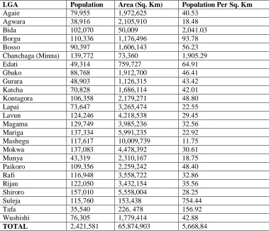
Niger state as one of the states in Nigeria is regionally placed at the north central part of Nigeria. It has 25 Local Government Areas (LGA), with population of 2, 421, 581 based on 1991 population census result, by National Population Commission. Table 2.1 shows 1991 population, area and population density of the state by LGAs. Every LGA has its own temperature readings relative to a particular period of time.
TABLE 2.1:1991 Population Census Result Showing Population, Area & Population Density of Niger State by LGAs
LGA Population Area (Sq. Km) Population Per Sq. Km
Agaie 79,955 1,972,625 40.53
Agwara 38,916 2,105,910 18.48
Bida 102,070 50,009 2,041.03
Borgu 110,336 1,176,496 93.78
Bosso 90,397 1,606,143 56.23
Chanchaga (Minna) 139,772 73,360 1,905.29
Edati 49,314 759,727 64.91
Gbako 88,768 1,912,700 46.41
Gurara 48,903 1,126,315 43.42
Katcha 70,828 1,686,114 42.01
Kontagora 106,358 2,179,271 48.80
Lapai 73,647 3,265,474 22.55
Lavun 124,246 4,218,538 29.45
Magama 129,749 3,985,236 32.56
Mariga 137,334 5,991,235 22.92
Mashegu 117,617 10,009,739 11.75
Mokwa 137,083 4,478,392 30.61
Munya 43,319 2,310,167 18.75
Paikoro 109,356 2,259,242 48.40
Rafi 116,948 3,558,722 32.86
Rijau 122,050 3,432,154 35.56
Shiroro 157,010 5,558,004 28.25
Suleja 115,760 153,438 754.44
Tafa 35,540 226, 478 156.92
Wushishi 76,305 1,779,414 42.88
TOTAL 2,421,581 65,874,903 5,668,84
III. TEMPERATURE SCALE
Holman [2] viewed thermodynamics as the study of energy and its transformation. Intuitively, the physical meaning of temperature is that it describes whether a body is hot or cold. For example, we touch a block of metal at 1200F and conclude that it is hotter than a block of ice. The reason for this conclusion is that the hot block of metal gives up heat energy to the hand whereas the cold block of ice extracts energy. Notice that this intuitive concept of temperature is based upon energy-transfer process that we might simply describe as heat exchange. It might therefore be possible to conclude that if two bodies at the same temperature are brought into contact no heat will be exchanged between the two. The two temperature scales normally employed for measurement purposes are the FAHRENHEIT and CELSIUS scales. These scales are based on a specification of the number of increments between the freezing point and the boiling point of water at standard atmospheric pressure. The Celsius scale has 100 units between these points, whereas the Fahrenheit scale has 180 units. The zero points on the scales are arbitrary. The absolute Celsius is called Kelvin scale and the absolute Fahrenheit scale is termed the Rankine scale, all this is known from the second law of thermodynamics, which serves to define an absolute thermodynamics temperature scale having only positive value. The Zero points on both absolute scales represent the same physical state, and the ratio of two values is the same regardless of the scale used. That is,
(Rankine) =
(Kelvin)
The boiling point of water is arbitrarily taken as 1000 on the Celsius scale and 2120 on the Fahrenheit scale.
TABLE 3.1: Relationship between Temperature Scales 0
K 0C 0F 0R
2273.16 2000 3632 4091.69
1773.16 1500 2732 3191.69
1273.16 1000 1832 2291.69
773.16 500 932 1391.69
673.16 400 752 1211.69
573.16 300 572 1031.69
473.16 200 392 851.69
373.16 100 212.0 671.69
273.16 0 32.0 491.69
233.16 -40 -40 419.69
173.16 -100 -148 311.69
From table 3.1, it is evident that the following relations apply:
0
F = 32.0 + 9/5 0C
0
R = 9/5 0K
0
R = 0F + 459.69
0
K = 0C + 273.16
To perform a measurement of temperature it is necessary to set up standards, which may be employed for calibration of various thermometer devices. The boiling and freezing points of water are two such standards, but they certainly do not encompass the whole range of temperatures of interest in experimental measurements. The international temperature scale of 1948 serves to set up standard check points over a wide range of temperature.
III.I DIURNAL TEMPERATURE VARIATIONS AND TEMPERATURE IN TROPICAL REGION
generally expressed as the mean diurnal range, indicating the difference between daily minimum and maximum temperatures. Factors which control the mean diurnal range are (1) Continental factor (2) Elevation (3) Cloudiness. Temperatures always go down with elevation, but the rate of the decrease, the lapse rate is far from uniform [3]. It does not only vary with cloudiness and, therefore, in many areas with the seasons, and between day and night, but also depends on the prevailing topography of the highlands. The temperature zone is one of the different belts recognized near the equator; others are the lowlands zone, the cold zone, the next zone, the frost zone. From about 500m to approximately 2000m above sea level the temperatures are considerably lower than in the low lands. The annual means temperature in this “tierra templada” which is Latin America varies between 160c and 240c.
III.II PHYSIOLOGICAL TEMPERATURE
The temperature, as experienced by living organism in general, and by human beings in particular, depends mainly on the rate of heat loss from the body. The human body is kept at a constant temperature of 36.70c, and defense mechanism prevents excessive loss of heat or too much heat absorption. Under warm conditions, heat disposal takes place mainly from the skin and the lungs, but, if this is not sufficient, it is greatly released by evaporation of body fluids in the form of perspiration from the skin. Physiological temperature does not depend only on the temperature of the air, but also on the efficiency and speed of evaporation, which is controlled by a number of other factors, such as (1) humidity (2) circulation of air around the body (3) direct exposure to solar radiation. Hitherto, any estimate that is based on 1 year temperature differences cannot be represented in terms of 1 year differences only because, monitoring data typically have missing values and cannot be represented in terms of 1 year differences only [4]. For example, if a time series of yearly temperature observation at a certain spatial sampling location has a missing data-item, then two 1 year differences will be left undefined when we do the differencing. Therefore, if the ith observed temperature corresponds to location xi and time ti, and if the previous observation at the same location xi occurred at time ti-ki, then we define
di = T (xi, ti) – T (xi, ti – ki) where
di = the observed temperature difference xi = the location of difference observation i ti = the time of difference observation i ki = the time of previous observation i
IV. METHODOLOGY
The data used in carrying out the modeling of temperature differences as presented in this paper were got from some locations in Niger state. The data were average daily minimum and maximum temperatures at three locations for year 1998 and year 1999. Year 1998 and year 1999 were chosen for this experiment due to so many factors. The model was set up using regression analysis, graphs, gathered data, and simulation approach using C++ programming language.
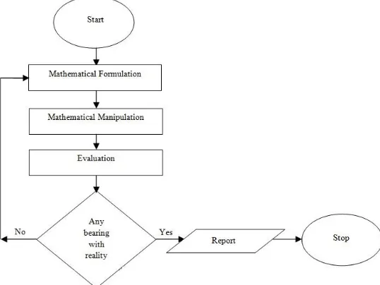
Fig. 4.1 is a flowchart representation of modeling methodology. After the identification of problem, mathematical formulation and manipulation are carried out on the problem, this leads to evaluation of the model, i.e. testing using data and finally, report is given if and only if the previous charts are correct.
TABLE 4.1: Year 1998 and Year 1999 Average Daily Minimum Temperature by Month in Three Locations in Niger State
Bida NCRI Minna
Month Year 1998 Year 1999 Year 1998 Year 1999 Year 1998 Year 1999
January 21.5 21.6 16.9 17.1 29.5
February 20.3 24.3 20.5 20.1 29.1
March 27.1 26.8 23.3 25.0 29.9
April 23.8 22.9 26.7 23.2 28.0 27.4
May 25.0 22.8 24.9 23.1 24.9 29.9
June 24.5 22.3 23.8 22.8 23.8 32.5
July 24.1 22.9 23.5 23.2 22.7 27.4
August 23.4 22.8 23.6 23.1 24.2 29.9
September 23.4 22.3 23.4 22.8 25.8 32.5
October 23.5 32.0 23.6 32.1 27.5
November 21.9 22.0 20.4 21.0 29.5 24.6
December 21.0 22.3 29.7
TABLE 4.2: Year 1998 and Year 1999 Average Daily Maximum Temperature by Month in Three Locations in Niger State
Bida NCRI Minna
Month Year 1998 Year 1999 Year 1998 Year 1999 Year 1998 Year 1999
January 35.4 38.6 35.2 35.3 31.4
February 39.6 37.5 40.1 37.3 31.8
March 39.1 38.1 40.0 38.0 32.1
April 38.7 39.0 32.4
May 34.4 34.4 31.7
June 32.8 33.6 33.7
July 31.0 30.3 31.5 31.1 30.9 32.4
August 29.8 29.8 30.5 30.3 26.1 33.2
September 30.7 30.1 31.3 30.7 30.9 33.0
October 32.4 32.9 32.1 32.9 24.1
November 36.2 35.3 35.7 36.0 34.6 34.1
December 35.0 34.8 32.4
V. THE MODEL
In this modeling, we applied the method of least squares [5] for a best fit. From the available data, we resolved at the following model:
Y = β0 + β1X (5.1)
D(x, t) = T(x, t) – T(x, t-1) (5.2)
Model (5.1) is the linear model for minimum and maximum temperature and model (5.2) is the model for temperature differences.
The model for minimum temperature for year 1998 is calculated thus:
∑ ̅̅̅
∑ ̅
∑ ̅
So, = 8.92
So from,
<β1=
and <β0 = ̅ ̅
= 69.06
The model is: ŷ0 = 69.06 + (-1.481 X0) (5.3)
The model for minimum temperature for year 1999 is calculated thus:
∑ ̅̅̅
∑ ̅̅̅ ̅̅̅
∑ ̅
∑ ̅
So, = 8.92
So from,
<β1=
and <β0 = ̅ ̅
= 8.22
The model is: ŷ0 = 8.22 + (0.45 X0) (5.4)
The model for maximum temperature for year 1998 is calculated thus:
∑ ̅̅̅
∑ ̅̅̅ ̅̅̅
∑ ̅
∑ ̅
So, = 8.92
So from,
<β1=
and <β0 = ̅ ̅
= 85.91
The model is: ŷ1 = 85.91 + (-1.688 X1) (5.5)
The model for maximum temperature for year 1999 is calculated thus:
∑ ̅̅̅
∑ ̅̅̅ ̅̅̅
∑ ̅
∑ ̅
So, = 8.92
So from,
<β1=
and <β0 = ̅ ̅
= 57.04
The model is: ŷ1 = 57.04 + (-0.75 X1) (5.6)
X is the explanatory variable which predicts the expected response value Y
The C++ program for the model to find the difference between the maximum temperature by month for year 1998 and //1999 is written as follows.
#include <iostream>
//This C++ program finds the difference between the maximum temperature by month for year 1998 and //1999 //include <math>
using namespace std; main()
{
float a= 85.91, b= -1, 688, c= 57.04, d= -0.75, x0, Y1, Y2; cout<<“Enter the days x0, for maximum temperature, 1998.\n”; cin>>x0;
cout<<”\n”;
cout<<”Enter the days x0, for maximum temperature, 1999.\n”; cin>>x0;
Y1= a + (b*(x0)); cout<<”\n”;
//This finds the output from x0.
cout<<”Maximum temperature data equivalent x0= = = = = = = =”<<Y1; cout<<”\n”;
Y2= c + (d * (x0)); cout<<”\n”;
//This finds the output from x1.
cout<<”Maximum temperature data equivalent for entered x0= = = = = = = =”<<Y2; cout<<”\n”;
float result = Y2 – Y1; cout<<”\n”;
//This produces their difference. cout<<”Their difference= = = = = = = =”<<result; cin>>x0;
The C++ program for the model to find the difference between the minimum temperature by month for year 1998 and //1999 is written as follows.
#include <iostream>
//This C++ program finds the difference between the minimum temperature by month for year 1998 and //1999 //include <math>
using namespace std; main()
{
float a= 69.06, b= -1, 481, c= 8.22, d= 0.45, x0, Y1, Y2; cout<<“Enter the days x0, for minimum temperature, 1998.\n”; cin>>x0;
cout<<”\n”;
cout<<”Enter the days x0, for minimum temperature, 1999.\n”;
cin>>x0; Y1= a + (b*(x0)); cout<<”\n”;
//This finds the output from x0.
cout<<”Minimum temperature data equivalent x0= = = = = = = =”<<Y1; cout<<”\n”;
Y2= c + (d * (x0)); cout<<”\n”;
//This finds the output from x1.
cout<<”Minimum temperature data equivalent for entered x0= = = = = = = =”<<Y2; cout<<”\n”;
float result = Y2 – Y1; cout<<”\n”;
//This produces their difference. cout<<”Their difference= = = = = = = =”<<result; cin>>x0;
return 0; }
VI. RESULTS AND DISCUSSIONS
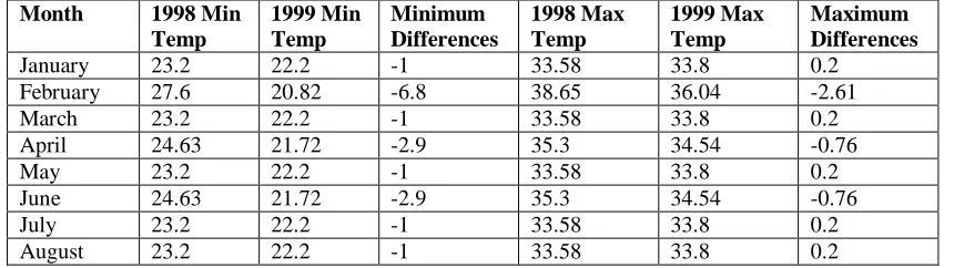
There are no fixed or permanent dividing lines between facts about a system, and the beliefs held about a system or situation. Models are theories, laws, equations or beliefs which state things about the problem in hand and assist in our understanding of it. Analyzed on table 6.1 is the difference in minimum and maximum temperature of the modeled data for year 1998 and year 1999. As it is analyzed in the table, trends in temperature data brings about differences in temperature, typical with Bida as the test location. Figures 6.1 and 6.2 are the C++ program snapshots of minimum and maximum modeled temperature data, year 1998 and year 1999 while figures 6.3 and 6.4 represents the line interpretation of minimum and maximum temperature differences, year 1998 and year 1999 respectively.
TABLE 6.1: Minimum/Maximum Temperature Differences
Month 1998 Min Temp 1999 Min Temp Minimum Differences 1998 Max Temp 1999 Max Temp Maximum Differences
January 23.2 22.2 -1 33.58 33.8 0.2
February 27.6 20.82 -6.8 38.65 36.04 -2.61
March 23.2 22.2 -1 33.58 33.8 0.2
April 24.63 21.72 -2.9 35.3 34.54 -0.76
May 23.2 22.2 -1 33.58 33.8 0.2
June 24.63 21.72 -2.9 35.3 34.54 -0.76
July 23.2 22.2 -1 33.58 33.8 0.2
September 24.63 21.72 -2.9 35.3 34.54 -0.76
October 23.2 22.2 -1 33.58 33.8 0.2
November 24.63 21.72 -2.9 35.3 34.54 -0.76
December 23.2 22.2 -1 33.58 33.8 0.2
VII. CONCLUSION
Modeling has come along way in representing physical systems mathematically, and this paper was all about predicting differences in temperature data by modeling, of which benefits to living things, agriculture, and environment cannot be overemphasized. Having put into consideration all the necessary conditions that can affect variation in temperature data and the effect of such variation, we are sure that the temperature differences model through the graph representations has successfully ease temperature prediction purposes, provided the data collected is accurately analyzed with the explanatory variables accurately applied. The Niger State Agricultural Development Project (NSADP) temperature data collected was used throughout this research work.
REFERENCES
[1]. Nieuwolt, S. Tropical climatology, an introduction to the climates of the low latitudes, John Wiley and Sons, Ltd., New York, 1977.
[2]. Holman, J.P., Thermodynamics, John Wiley and Sons, Ltd., New York, 1985.
[3]. Rodriguez-Iturbe, I. and Mejia, J.M. The design of rainfall networks in time and space. Water Resources Research, 10(4), 713-728, 1974.
[4]. Knut, S. and Paul, S. Time trend Estimation for a Geographical Region, Theory and Methods. Journal of the America Statistical Association, Volume 91, Issue 434, June 1996.