Plates Bending Analysis Using Finite Element Method
K Rajendraprasad1, J.Varaprasad2
1
P.G. Scholar, 2 Guide, Head of the Department
1,2
BRANCH : Structural Engineering
1,2
SVR Engineering College NANDYAL
EMAIL.ID : [email protected], [email protected].
ABSTRACT:
Advent of approximate Numerical methods for the analysis of complicated problems has provided platform to the researchers and engineers. Towards this, advent of digital computer has increased exponentially the useful application of approximate methods. Using Finite Element Method, an approximate method, the analysis over the bending of plate has been done using four noded isoperimetric elements in this thesis The element properties and some essential criterions like convergence, compatibility and geometric invariance has been described. Numerical difficulties like locking phenomenon and stress smoothing technique has also been
overcome with Hinton & Campbell
technique [1974]. Thin plate theory i.e. Kirchoff‟s and Mindlin theory along with Finite Element Formulation has been described. Variation of deflection and moments at various points on the plates with the variation of percentage error in respect of each variable have been shown in graphical form with the variation of number of elements. Effect of mess fineness and element aspect ratio on the deflection as well as the stress resultants have been studied for various sizes of plates using Lisa/Ansys.
Keywords:-Bending Analysis, Finite
Element Method, Mindlin’s Theory
INTRODUCTION
The present study is devoted to analyze plate with various boundary
conditions. A finite element based software package has been developed which can solve plates of any arbitrary shape. During last three decades finite element procedures have also been successfully employed to solve these problems. As a numerical solution to the problem a number of finite element models have been proposed. Of these, the present study will use
four-nodded isoperimetric plate elements.
Detailed mathematical formulation has been presented in the following sections. The
numerical difficulties like locking
phenomenon, local stress smoothing has also been described. Vast literature based on classical plate theory exists for solving these commonly used structural elements. But the classical theory is very cumbersome for the arbitrary shape of plates and cannot be formulated. The three methods that are used are as
1. Functional approximation
2. Finite difference method
3. Finite element method
Out of these three methods Finite Element Method is mostly used because of its accuracy and simplicity than that of other two methods.
In functional approximation, a set of
independent functions satisfying the
boundary conditions is chosen and a linear combination of a finite number of them is taken to approximately specify the field variable at any point.
.
field variable is represented by the discrete value of the variables at the nodes.
In the finite element method the body is divided into a number of smaller elements which are called finite elements. For each element equilibrium equation is formulated and then combined for whole structure and the simultaneous equations are solved for unknowns.
OBJECTIVES
The present study envisages fulfilling the following objectives:
1. To use four-noded isoperimetric plate element to analyze plates.
2. To develop a finite element based software package for analyzing plate bending problems.
3. Various possible boundary conditions for various shapes of plates will be investigated.
4. Results from analysis using above two plate element will be compared to see their relative performance with respect to classical solution.
5. To study the effect of mess fineness and element aspect ratio on finite element solution.
FINITE ELEMENT METHOD
Finite element analysis is a method for numerical solution of field problems. A field problem requires that determination of spatial distribution of one or more independent variables. Mathematically, a field problem is described by differential equations or by integral expressions.
The word finite distinguishes these pieces
from infinitesimal elements used in
calculus. In each finite element a field quantity is allowed to have only a simple spatial variation. The actual variation in the region spanned by an element is more
complicated. So, FEA provides an
approximate solution. The particular
arrangement of an element is called mess. Numerically an FEA mess is represented by a system of algebraic equations to be solved for unknowns at the nodes. The solution for
the nodal quantities when combined with the assumed field in any given element, completely determines the spatial variations of the field in that element.
ADVANTAGES OF FEA
1. FEA is applicable to all types of
problem.
2. There is no geometric restriction.
3. Boundary conditions and loading are not
restricted.
4. Material properties are not restricted to isotropy and may change from one element to other or even within an element.
5. The components have different
mathematical behaviour and different
mathematical descriptions, can be
combined.
The FEA also suffers from mainly two types
of errors, i.e. modeling error and
discretization error. The modeling error can be reduced by improving the models and discretization error can be reduced by increasing elements.
THEORY OF ELEMENT PROPERTIES Isoperimetric element
For the element description, shape functions are used to interpolate both the displacement field and element geometry. That is, displacement of a point within an element can be expressed in terms of nodal degree of freedom and shape function
N , which are the functions of referencecoordinates. Similarly the global
coordinates of a point within the element can be expressed in terms of global nodal positions and shape functions
N , which are also the functions of reference coordinates. Symbolically1. Nodal degree of freedom
d defines2. Nodal coordinates
c defines coordinates
x,y,z
of a point within the element; i.e.
x,y,z
T
N
c .The shape function matrices
N and
N are the functions ofr,sandt. An element iscalled isoperimetric, if
N and
N are identical. If
N is of lower degree than
N , the element is called subparametric and if
N is of higher degree than
N , the element is called super parametric.Bilinear quadrilateral (Q4)
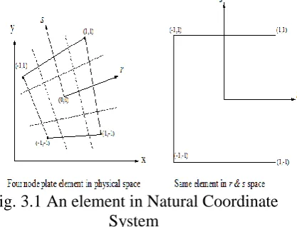
This plane element is a
generalisation of rectangular Q4 element that removes the restriction to rectangular shape. The locking effect also appears in this element. In this, in physical space, reference coordinates r&s need not be orthogonal unlike rectangular Q4 element and need not be parallel to Cartesian coordinates x and y. Element sides having coordinates r1and s1 are bisected by axes r&sregardless of the shape or physical size of the element and regardless of its orientation in Cartesian coordinates. The point rs0is normally the element centre, but in general it is not the centroid of the physical element. The displacements are directed parallel to Cartesian coordinates, not parallel to local coordinatesr&s.
Fig. 3.1 An element in Natural Coordinate System
STATIC CONDENSATION
The internal nodes of any element do not connect with any node of adjoining
elements in the assemblage. So, the degrees of freedom of such nodes do not appear in the compatibility conditions that are used to formulate the overall equations for the structure. The internal degrees of freedom can be eliminated from the equilibrium equations of each element so that these extra unknowns do not increase the number of overall equations.
SOME ESSENTIAL CRITERIA Convergence requirements
The finite element method provides a numerical solution to a complex problem. It is expected that the solution must converge to exact solution under certain circumstances. Hence as the mess is made finer, the solution should converge to the correct result and this would be achieved if the three conditions are satisfied by assumed displacement functions.
1. The displacement function must be
continuous within the element and it can be satisfied by choosing polynomials for the displacement model.
2. The element displacement function must
be capable of representing rigid body displacements of the elements. That is when nodes are given such displacements corresponding to a rigid body motion, the element should not experience any strain.
3. The element displacement function must
be capable of representing constant strain states within element. For one, two or three dimensional elasticity problems the linear terms present in the polynomial satisfy the requirement. However, in the case of beam, plate and shell elements, this condition will be referred to as „constant curvature‟ instead of „constant strains‟.
Geometric invariance
Besides the convergence and
compatibility requirements, another
isotropy or geometric invariance. Geometric invariance is achieved if the polynomial includes all the terms i.e. polynomial is complete one. Invariance may also be achieved if polynomial is balanced, in case all the terms can not be included.
For example
xy a y a x a a
u 1 2 3 4 (3.1)
It can be achieved from the Pascal triangle for two dimensional elements.
NUMERICAL DIFFICULTIES Locking phenomenon (URI & SRI)
A locking phenomenon is a well-known event in finite element applications. It may be due to shear locking or membrane locking, which results when proper order of integration is used to find out the stiffness matrix. When Q4 element bents, it displays shear strain as well as bending strain. When a Q4 element is bent, its top and bottom sides remain straight, and each node has only horizontal displacement of certain magnitude.
Inclusion of transverse shear strains, in
the equations presents computational
difficulties when span to thickness ratio of plate is large.
For thin plates, the transverse shear strains are negligible and consequently the element stiffness matrix becomes stiff and yields erroneous results for the generalized displacements. This phenomenon is known as shear locking, and it can be interpreted as being caused by the inclusion of the following constraint in the variational form (Averill & Reddy, 1992)
0
0
y w and
x w
y
x
(3.2)
If the plate is thick, the above condition does not satisfied and locking does not
occur. For thin plate the above constraints are valid but not satisfied in the numerical model. To avoid this locking phenomenon URI (uniformly reduced integration) or SRI (selective reduced integration) technique are used. When four noded elements is used one point gauss rule should be used for shear energy terms while two point gauss rule should be used for all other terms.
Stress smoothing technique
Using displacement method, it was reported in the literature that the stresses obtained from finite element solutions are discontinuous between elements.
Hinton & Campbell (1974) devised a local stress smoothing technique which is a natural method of sampling stresses in finite element using reduced integration. Here local smoothing is done by a bilinear extrapolation of the stress values computed at the Gauss points.
IV III II I
2 3 1 2 1 2
3 1 2 1
2 1 2
3 1 2 1 2
3 1
2 3 1 2 1 2
3 1 2 1
2 1 2
3 1 2 1 2
3 1
4 3 2 1
(3.3)
Where, 1 to 4 are the smoothed nodal
values and I to IV are the stresses at the 2 x 2 Gauss points.
THIN PLATE THEORY Love and Kirchhoff theory
1. After application of the external load, a lineal element of the plate normal to the mid surface
(a) Undergoes at most a translation and
rotation, which indicates that lineal element through the thickness does not elongate or contract and
(b) Remains normal to the deformed
mid-surface. It shows that shear strains xz
and yz becomes zero.
2. The stresses normal to the plate can be neglected, i.e. z 0.
Basic Relationships
The stresses in thin plate vary linearly across the thickness and hence the stresses resultants can be computed as
if u, v and w be the displacements at any point (x, y, z) then the displacement u and v across the thickness can be expressed in
terms of the displacement w as
y w z v x w z u
(3.5)
the strain distribution is given by
x x zk x w z x u
22
y y zk y w z y v
22
xy xy zk y x w z x v y u
2 2
(3.6)
and the shear strains xz yz 0. Thus problem reduced to plane stress problem.
The general constitutive law for plane stress
is given by
xy y x xy y x C C C C C C C C C 33 32 31 23 22 21 13 12 11
Conveniently in the case of plate,
M can be written in place of
.Hence xy y x xy y x k k k C C C C C C C C C h M M M 33 32 31 23 22 21 13 12 11 3 12 (3.7)
i.e.
M
Cf
kcIn case of isotropic plates, the constitutive matrix is given by,
2 1 0 0 0 1 0 1 ) 1 ( 12 2 3 Eh Cf (3.8) Mindlin’s Theory
This theory includes shear
deformations in the plates, which was not considered in the Kirchhoff‟s theory. There are three assumptions in the Mindlin‟s theory of plates as given below:
1. The deflections of plate,w, are small. 2. Normal to the plate mid surface before
deformation remains straight but is not
necessarily normal to it after
deformation.
3. Stresses normal to the mid surface are negligible.
The average shear deformation, xandy
are given by y w x w x y y x
(3.9)
the strain energy for the thin plate due to
shear be given as
Where, G modulus of rigidity and is equal
toE/2(1).
Putting the value of x and y from
get:
The expression for the strain energy due to bending of an isotropic plate can be obtained as
The total strain energy is given by
U Ub Us Basic Relationships
The shear stresses xz&yz and shear
deformations x&y are related as
y x yz xz C C C C 55 54 45 44 the average shear deformations x &yare constant all over the thickness and allowing for warping of the x-section, the stress resultant Qx&Qycan be computed as
Where, is numerical correction factor
used to represent the restraint of the x-section against warping. The value of commonly used is 5/6 but may be assumed between 2/3 for section having no restraint against warping and 1.0 for sections having complete restraint against warping.
The stress resultants
M & Q can be combined and for homogeneous plate it canbe expressed as:
y x xy y x y x xy y x k k k C C C C h C C C C C C C C C h Q Q M M M 55 54 45 44 33 32 31 23 22 21 13 12 11 3 0 0 0 0 0 0 0 0 0 0 0 0 12
For an isometric plate, using specific values of coefficient for the consecutive matrix, we get y x xy y x y x xy y x k k k ) ( Eh ) ( Eh Q Q M M M 0 0 1 2 0 0 0 0 0 0 0 0 0 0 0 0 2 1 0 0 0 1 0 1 1 12 2 3
In short the above relation can be written as
c s T f k C C Q M 0 0
FINITE ELEMENT FORMULATION FOR FOUR NODDED BILINEAR PLATE ELEMENT.
System of Coordinate Axes
Various coordinate system used in the present formulation are
a. Natural coordinate system
b. Local coordinate system
c. Global coordinate system
In natural coordinate system the axes are taken as r and s and the coordinates of elements are taken as unity.
Geometry Representation
Element Geometry and
Displacement Field: both the geometry of the element and displacement field is obtained using same polynomial functions (also called shape functions in FEM literature). Geometry is expressed by
i i ix N x
4 1 i i iy N y
4 1 (3.13)and displacement field is expressed as
4 1 i i iw N w i x i ix N
4 1 yi i iy N
4
1
(3.14)
Where, the shape function for any ith node is given by
Ni
1rri
1ssi
4 1
Displacement Vector
The typical nodal displacement
vector for an element is given as
1 x1 y1 2 x2 y2 3 x3 y3 4 x4 y4
T
w w
w w
d (3.15)
The shape function used for describing the geometry of the element and displacement variation are expressed in natural coordinate
(r,s). The relationship between two
coordinate systems can be computed by using the chain rule of partial differentiation and is given below:
y x J y x s y s x r y r x s rWhere, [J] is Jacobian matrix. Hence, the derivatives with respect to Cartesian coordinate system can be given as
s r J y x 1 ] [
Jacobian matrix for four nodded element can be given as
4 4 3 3 2 2 1 1 3 4 3 2 1 4 2 1 y x y x y x y x s N s N s N s N r N r N r N r N J s N s N s N s N r N r N r N r N J y N y N y N y N x N x N x N x N 4 3 2 1 4 3 2 1 1 4 3 2 1 4 3 2 1 (3.16)
3.9.4 Strain displacement matrix [B] The element curvature and shear
deformation
pand nodal displacement
d are related as
p
B
dFor getting the each terms of
pdifferentiate Eq. (3.14) w. r. t. x and y. we get 4 1 i i yi x x N k 4 1 4 1 i i xi i i yi xy x N y N
k
4 1 4 1 i i i yi i i x N x N
4 1 4 1 i i i xi i i y N y N (3.17)
Where
y N x
Ni i
and are to be computed
from Eq. (3.16)
Eq. (3.17) shows that the elements of vector
p are expressed in terms of nodal displacements, w,θxi andθyi.Hence 4 4 1 1 1 .... .... y x y x y x xy y x
p k B
k k (3.18)
This equation can be expressed as
ii i
p
B d
4
1
(3.19)
Where 4 , 3 , 2 , 1 0 0 0 0 0 0 0 i i i i i i i i i i N y N N x N y N x N y N x N B (3.20) and yi xi i i d ] [
The stress resultant
pcan be expressed interms of nodal displacements as following
p p
y x xy y x p C Q Q M M M i i i
p B d
C
4
1
. (3.21)
or
p
C
pB
d
(3.22)Where,
4 1 i i B
B (3.23)
Element stiffness matrix
The element stiffness matrix
k is given by k B C B dx dy A
p T
(3.24)
The above expression in local coordinate is written as
k B C B J dr ds
A
p T
The matrix
k can be written as sum of bending and shear contributions.
k k b k s (3.26) Substituting
k for
B C p BT
in Eq.(3.25), the stiffness matrix is given by
1 1 1 1 ds dr J k k
1 1 1 1 ds dr J k kk b s (3.27)
Gauss quadrature rule is used to compute the stiffness matrix
k .Element nodal load vector
The nodal load
Qi at the node i for a uniformly distributed load q is given by Jdrds
q N M M F Q A i y x Z i 0 0 (3.28)
The element load vector {Q} can be calculated by combining the nodal load
vectors
Qi as 4 1 4 1 4 3 2 1 12 11 10 9 8 7 6 5 4 3 2 1 0 0 0 0 0 0 0 0 i j j i N N N N J W W q Q Q Q Q Q Q Q Q Q Q Q Q Q (3.29)
Gauss quadrature of 2x2 sampling points is used to evaluate Eq. 3.29
3.9 RECTANGULAR AND CIRCULAR PLATE THEORY FOR ANALYTICAL SOLUTION
The equation for vertical deflection and moment resultants i.e. Mx, My, and Mxy are given in the book „Theory of Plates and Shells‟ by S. Timoshenko and S. W. Krieger second edition (1959). These equations for rectangular simply supported plates are given as
.. , , m n ,,...mn b y n sin a x m sin b n a m a D w 5 3
1 135
2 2 2 2 2 4
1
(3.30) Where mn q dy dx b y n sin a x m sin ab q a a b mn 2 0 0 0 0 16 4
(3.31)and m and n are odd integers. If m and n are both even numbers then amn 0.
Moment Mx is represented as
b y n sin a x m sin b n a m mn b n a m q M ... , , m n ,,.... x 5 3 1 135
2 2 2 2 2 2 2 2 2 2 2 2 2 2 0 16 (3.32) b y n sin a x m sin b n a m mn b n a m q M ... , ,
m n ,,....
y 5 3
1 135 2
2 2 2 2 2 2 2 2 2 2 2 2 2 0 16 (3.34) The defection equation for simply supported circular plate is
2 2
2 2
1 5
64D a r
r a q w
(3.35)
Radial moment Mr and Mt is given as
3 2 2
16 a r
q
Mr (3.36)
3 1 3
16
2 2
q a r
Mt (3.37)
The deflection and moments for clamped circular plate are given as
D r a q w 64 2 2 2 (3.38)
1 3
16 2 2 r a q
Mr (3.39)
1 1 3
162
2
q a r
Mt (3.40)
Where r is the radial distance of any point from centre of the plate and a is the radius of the circular plate.
DESCRIPTION GENERAL
The present study employs the Computer program PLATEFEM as provided by Krishnamoorthy (1994). The program is
written in the standard FORTRAN
problems. An effective column storage scheme is adapted to store the global
stiffness matrix elements as one
dimensional array SK. This program is something different from a finite element program SAP in view of their capability to print the shear components , which is not included in SAP. The various subroutines are subroutine PASSIN, FELIB, COLUMH, CADNUM, PASSEM, PASOLV, PASLOD and DISP.
MAIN PROGRAM
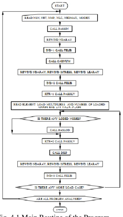
The main program controls the various tasks of the program. It reads the control information namely the number of structure nodes (NSN), number of element types (NET), number of material property group (NMP) and number of load cases (NLC). It stores the dataset of all variables in the master array A and NA. The execution stops if the sum total of dimensions of all the variables i.e. floats or integer exceeds that of the master arrays A and NA. Three scratch files ISTRESS, NDARAY and LEARAY to store stress displacement matrix, degree of freedom and number of elements at particular nodes respectively. After reading the data execution is done in three segments according to the value of flag IND. The flow chart of main routine is given in Fig. 4.1
Fig. 4.1 Main Routine of the Program Subroutine PASSIN
Subroutine COLUMH
The subroutine COLUMH computes the height of each column of the global stiffness matrix. The column height refers to the number of elements in each column below the sky line and above the leading diagonal excluding the diagonal element of the global stiffness matrix.
Subroutine CADNUM
Subroutine CADNUM calculates the
number of the diagonal element of the global stiffness matrix. The numbers of the diagonal elements of the global stiffness matrix are stored in a separate array called NDS. The number of diagonal element is obtained by adding the preceding column height one to its diagonal number, the
number of first diagonal element being taken as 1. The flow chart is given below.
Subroutine PASSEM
Subroutine PASSEM is called at the second stage i.e. at IND=2, by each element shape routine. It assembles the element stiffness matrix to global stiffness matrix in the form of one dimensional array SK. The flow chart of this subroutine is given below
Subroutine PASOLV
Subroutine PASLOD
The subroutine PASLOD is called by main routine for each load case to read and add the concentrated load in the direction of each degree of freedom of the node. These lodes are added to the structure load vector from the element shapes.
Subroutine DISP
Subroutine DISP prints out the
displacements of each node. The
displacement of each node is computed from the global displacement vector
TYPICAL DETAILS OF INPUT DATA This section describes a sample input for analysis of plates using computer program PLATEFEM. A typical input data has been presented in Appendix A. Herein
the brief description of variables along with their format is presented.
OUTPUT DETAILS
The output of program gives problem title, the controlling parameters like, number of structure nodes, element
types, material groups and loading
and the coordinates for each node is printed. The number of total equations and the total number of elements in global stiffness matrix are printed.
This program also prints the
deflection at each node along three degrees of freedom i.e. one vertical deflection w and two rotations and . At each node the moments i.e. Mx, My and Mxy are also printed. The constant shear force for each element is also printed in output file. A sample of output file is shown in Appendix A.
PROGRAM FOR ANALYTICAL
SOLUTION
For analytical solution a FORTRAN program has been written for simply supported rectangular plate and another program in FORTRAN is written in for simply supported and fixed circular plate. This program prints deflection and moments at any location as per requirements. The units of output file depend upon the units used in input data. These programs are shown in Appendix C.
RESULTS AND DISCUSSION
In this chapter the problem for the
validation of programme has been
described. The results obtained from computer programme are compared with the solution obtained from analytical solution. The exact analytical solution procedure for plates of Timoshenko and Krieger (1959) has been used.
PROBLEM FOR VALIDATION OF
COMPUTER PROGRAM
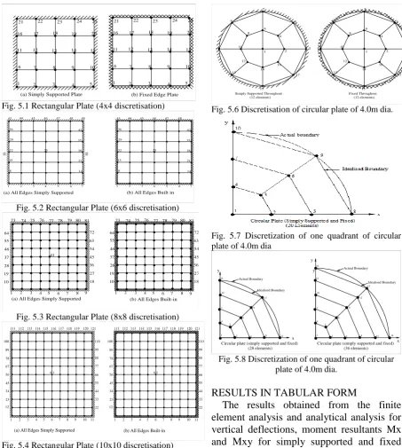
A simply supported square plate of 4.0m dimension is taken and analysed for the vertical deflection (w) and moments Mx, My, and Mxy. The thickness of plate is 0.12m and modulus of elasticity of material is taken as 2x10⁷ kN/m2. This result has been compared with the results obtained from the exact solution and it was found that computer programme is giving results close to those obtained from exact solution method. The discretisation scheme used is
shown in Fig. 5.1 and results for w, Mx and Mxy are shown in Table 1(a) & (b).
PLATE PROBLEMS ANALYSED
For further analysis the rectangular plate of least dimension 4.0m with thickness 0.12m are taken with simply supported and fix boundary conditions. Other dimension of rectangular plate is decided on the basis of aspect ratios, viz., 1.0, 1.2, 1.4, 1.6, 1.8 and 2.0. A set of circular plates of 4.0m diameter and thickness 0.12m are also analysed. The modulus of elasticity is taken as 2.0 x 10⁷ kN/m2.
Plate boundaries and support conditions The different plate boundaries which are taken for the analysis are square, rectangular and circular, with all edges simply supported and all edges built-in. The plate boundaries are shown in Figures from Fig. 1 to Fig. 8. Support conditions for rectangular plate are shown in Fig. 5.1-5.4. Fig. 5.5 shows the one quadrant of the plate for both simply supported and fixed boundary. Fig. 6 shows the circular boundary for both simply supported and fixed boundary conditions.
Discretization scheme
1 2 3 6 11 16 7 8 12 17 13 18 21 22 23
4 5 9 10 14 19 15 20 24 25
1 2 3 4 5
17 6 7 11 16 12 21 22 20 18 8 9 13 14 19 10 15 23 24 25
(a) Simply Supported Plate (b) Fixed Edge Plate
Fig. 5.1 Rectangular Plate (4x4 discretisation)
SS SS 25 35 28 21 14 7 6 5 4 3 2 1 8 15 22 29 36 42 48 47 46 45 44 43 49 48 47 45 44 43 42 46 36 35 29 25 28 22 21 15 14 8 7 6 5 4 3 2 1
(a) All Edges Simply Supported (b) All Edges Built in
Fig. 5.2 Rectangular Plate (6x6 discretisation)
19 1 10 2 3 28 37 46 55 73 64 75 74
4 5 6 7 41 27 18 8 9 63 54 45 36 76 77 78 79
72 81 80 19 2 1 10 3 28 37 46 55
4 5 6 7 73
64 75
74 76 77 78 79
8 9 81 80
(b) All Edges Built-in (a) All Edges Simply Supported
Fig. 5.3 Rectangular Plate (8x8 discretisation)
34 1 12 23 2 3 78 56 45 67 100 89
111 112 113
44
6 5
4 7 8 9 10 11 33 22 118 6 1 116 115 114 117 88 66 55 77 120 119 110 99 121 118 34 4 1 23 12 3
2 5 6 7 8 114 78 56 45 67 100 89
111112113
6 1 116 115 117
44
9 10 11 22 33 88 66 55 77 119120 99 121 110
(a) All Edges Simply Supported (b) All Edges Built-in
Fig. 5.4 Rectangular Plate (10x10 discretisation)
Fig. 5.5 Discretised figure of 4.0m x 4.8m size plate (one quadrant)
1 2 3
4 6 8 10 12 14 16 17 5 7 9 11 13 15 Simply Supported Throughout (12 elements) 11 Fixed Throughout (12 elements) 15 13 10 12 17 16 14 1 2 9 8 4 6 5 7 3
Fig. 5.6 Discretisation of circular plate of 4.0m dia.
Fig. 5.7 Discretization of one quadrant of circular plate of 4.0m dia
Circular plate (simply supported and fixed) (28 elements) 13 10 1 4 7 2 5 3 6 8 11 9 12 y x Circular plate (simply supported and fixed) (36 elements)
13
x 1 2
4 3
6 7 10
5 8 11 14
9 12 15 y y 16 Idealised Boundary Idealised Boundary Actual Boundary Actual Boundary
Fig. 5.8 Discretization of one quadrant of circular plate of 4.0m dia.
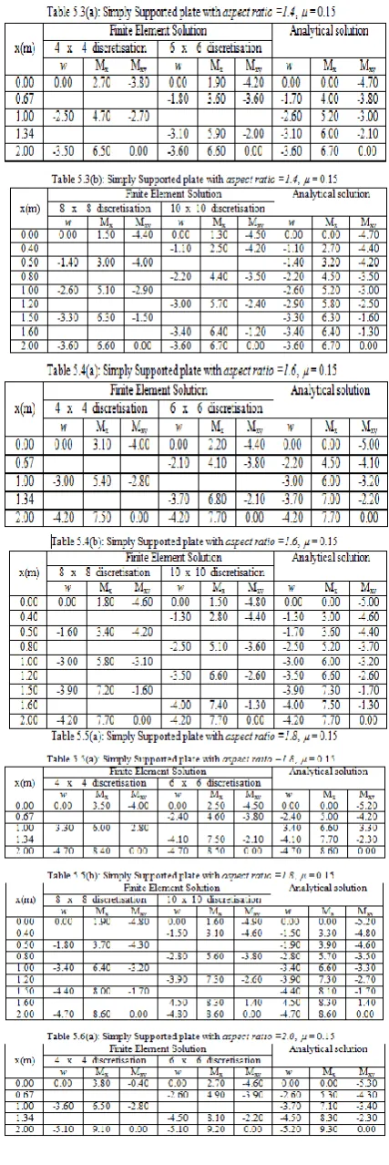
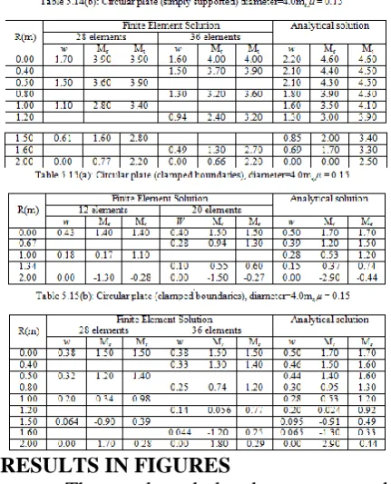
RESULTS IN TABULAR FORM
shown in Table 8 to Table 13. In Table14 &15 the vertical deflections and moment resultants Mr & Mt obtained from finite element solution and analytical solution are presented for circular plate with simply supported edges and fixed edges. The units used for vertical deflection (w), moment resultants Mx and Mxy, in case of rectangular plates and Mr and Mt in case of circular plates are millimetre (mm) and kN-m.
My is not presented here because in square plate My is same as Mx. For rectangular plates the maximum value of My is same as the value of Mx of a square plate of dimension same as the shorter dimension of rectangular plates.
Table 5.1(b): Simply Supported plate with aspect ratio = 1.0, = 0.15
Table 5.2(a): Simply Supported plate with aspect ratio =1.2, = 0.15
RESULTS IN FIGURES
The results tabulated are presented
in graphical form for variation of
deflections and moments along the central line of the square and circular plates only with simply supported and fix boundary conditions for the sake of convenience. Descriptions of Figures for deflection and moment patterns are given below from Fig. 5.9 to Fig. 5.19.
Variation of deflection
Fig. 5.9 shows the variation of vertical deflection w along central line in SS
rectangular plate with various
discretisations. It shows very close variation of finite element solution with analytical solution. Fig. 5.12 shows the variation of displacements along central line in fixed square plate. Fig. 5.14 represents the variation of vertical deflection along radius of simply supported circular plate. Fig. 5.17 shows the variation of deflection along the
radius of circular plate with fixed
boundaries. This graph represents that the deflections are close to analytical values but not tend to converge with increasing the number of elements.
Variation of Moment (Mx and Mxy)
Fig. 5.10 shows the variation of Mx along central line in SS rectangular plate with
different discretisation. This figure
represents the convergence of FEM value to analytical value with increasing the number of elements. Fig 5.13 represents the variation of moments Mx in fixed rectangular plate. For positive moment the value from FEM is very close to analytical value but for support moment these values differ considerably. Fig. 5.11 represents the variation of Mxy along the SS edge. This represents that the results from FEM converges to analytical solution with increasing the number of elements.
Variation of radial moment (Mr)
The variation of radial moment Mr along radius is presented in Fig 5.15. The results obtained from FEM are very near to analytical solution but to not fully converge with increasing the number of elements. Fig. 5.18 represents the variation of Mr along the radius of fix circular plate.
Variation of tangential moment (Mt)
Fig. 5.16 shows the variation of tangential moment Mt along radius in SS circular plate. The FE solution follow the same
pattern as exact solution but have
approximately uniform difference between the FEM values and exact values. Variation of Mt along radius of fixed circular plate is presented in Fig. 5.19.
Fig. 5.9 Variation of displacement w, along mid-line (Simply supported rectangular plate)
Variation of displacement at y=b/2
-2.5 -2 -1.5 -1 -0.5 0
0 0.5 value of X(m)1 1.5 2
De
fle
ct
io
n
(m
m
) FEM 16 elements
Fig. 5.10 Variation of Mx along mid-line
(Simply supported rectangular plate)
Fig. 5.11 Variation of moment about X-axis along edges
(Simply supported rectangular plate)
Fig. 5.12 Variation of w along mid-line (Clamped Rectangular plate)
Fig. 5.13 Variation of Mx along mid-line
(Clamped Rectangular plate)
Fig. 5.14 Variation of vertical deflection w along radius
(Simply supported circular plate)
Fig. 5.15 Variation of radial moment Mr, along
radius
(Simply supported circular plate)
Fig. 5.16 Variation of tangential moment Mt along
radius
(Simply supported circular plate)
Fig. 5.17 Variation of vertical deflection w along radius
(Fixed circular plate)
Fig. 5.18 Variation of radial moment Mr along radius
(Fixed circular plate)
Fig. 5.19 Variation of tangential moment along radius
(Fixed circular plate)
Variation of moment (Mxy) along the edges
-4 -3 -2 -1 0
0 0.5 1 1.5 2
Value of X(m)
M
om
en
t (
M
xy
) FEM 16 elements
FEM 36 elements FEM 64 elements FEM 100 elements Ana. Soln.
Variation of deflection along y=b/2
-0.8 -0.6 -0.4 -0.2 0
0 1 2
Value of X(m)
D
ef
le
ct
io
n
(m
m
) FEM 16 elements
FEM 36 elements FEM 64 elements FEM 100 elements Ana. soln.
Varation of moment along y=b/2
-5 -4 -3 -2 -1 0 1 2 3
0 0.5 1 1.5 2
Value of X(m )
Mo
me
nt
(Mx)
FEM 16 elem ents
FEM 36 elem ents
FEM 64 elem ents
FEM 100 elem ents
Ana. Soln.
Variation of displacements along radius
-2.5 -2 -1.5 -1 -0.5 0
0 0.5 1 1.5 2
Value of radius from centre (m)
D
ef
el
ct
io
n
(m
m
) FEM 12 elements
FEM 20 elements FEM 28 elements FEM 36 elements
Ana. Soln.
Variation of radial moment along radial direction
0 1 2 3 4 5
0 0.5 1 1.5 2
Radius (m)
R
ad
ia
l m
om
en
t
(M
r)
FEM 12 elements FEM 20 elements FEM 28 elements FEM 36 elements Ana. Soln.
Variation of tangential moment (Mt) along radius
1.5 2 2.5 3 3.5 4 4.5 5
0 0.5 1 1.5 2
Radius (m)
Ta
ng
en
tia
l m
om
en
t (
M
t)
FEM 12 elements FEM 20 elements FEM 28 elements FEM 36 elements Ana. Soln.
Variation of deflection along radius
-0.6 -0.4 -0.2 0
0 0.5 1 1.5 2
Radius (m)
D
ef
le
ct
io
n
(m
m
) FEM 12 elements
FEM 20 elements
FEM 28 elements
FEM 36 elements
Ana. Soln.
Variation of radial moment along radius
-3 -2 -1 0 1 2
0 0.5 1 1.5 2
Radius (m)
R
a
d
ia
l
m
o
m
e
n
t
(M
r)
FEM 12 elements FEM 20 elements FEM 28 elements FEM 36 elements Ana. Soln.
Variation of tangential moment along radius
-0.5 0 0.5 1 1.5 2
0 0.5 1 1.5 2
Radius (m)
Ta
n
g
e
n
ti
a
l
m
o
m
e
n
t
(M
t)
VARIATION OF VALUES AT SELECTED POINTS
The description of figures from Fig. 20 to Fig. 31 for the values of deflections and moments at particular points are given below.
Deflection variation
Fig. 5.20 shows the variation of deflection at the centre of SS rectangular plate with number of elements. This figure shows that
the FEM values converge to exact solution
with increasing the number of elements.
Fig. 5.23 represents the values of deflection at the centre of fixed rectangular plate. This figure represents the rapid convergence of deflection values obtained by FEM to exact analysis solution. Both values differ but not converge with increasing the number of elements. Fig. 5.29 represents the variation of vertical deflection at centre of the clamped circular plate. But here results are out of trends. The FEM results differ
increasingly from exact value with
increasing the number of elements. This may be due to approximate geometry and mess discretization technique adopted near the central zone.
Bending and torsion moments variation Fig. 5.21 represents that the value of Mx at the centre of SS rectangular plate fully converge with exact solution, for increasing the number of elements from 16 to 100. Fig. 5.24 represents the values of Mx at the centre of fixed rectangular plate and converges to exact value with increasing the number of elements. Fig. 5.25 represents the values of Mx at the support at central line in
fix edges rectangular plate. The
convergence of values is shown in the Figure. Fig. 5.22 represents the value of Mxy obtained from FEM at the corner node of SS rectangular plate converges with increasing the number of elements.
Variation of radial moment Mr
Fig. 5.27 represents the variation of Mr at the centre of SS circular plate. These values converge slowly with increasing the number of elements. Fig. 5.30 shows the variation of
Mr at the centre of clamped circular plate. Here the FEM results converge to exact value with increasing the number of elements.
Variation of tangential moment Mt
Fig. 5.28 represents the variation of Mt at the supports with the number of elements. This figure shows the convergence of FEM value to exact value with increasing the number of elements from 12 to 36. Fig. 5.31 shows the variation of Mr at support of clamped circular plate. The FEM result converges to exact value on increasing the number of elements.
CONCLUSIONS
On the basis of results obtained from
analysis the following significant
conclusions are drawn.
The study of rectangular and circular
shape plate with simply supported and fixed boundary conditions shows the
potentiality of computer program
developed especially to analyse the plates. This program is applicable to thin plates of any shape with all possible boundary conditions.
The difference in the results obtained
from FEM and exact solution, shows the effect of discretization and this type of error can be reduced by increasing the number of elements.
The results confirm the shear locking
effect in the Q4 element, which reduces with decreasing the size of elements. Because shear force is computed at the central Gauss point of the element and are constant throughout the element. Smaller elements show smaller shear forces and hence better results are obtained.
For fix boundaries the element shows their non usability for calculation of negative moments at supports.
FUTURE SCOPE OF STUDIES
The same analysis can be done using
eight noded, three noded and six noded isoparametric element, which confirm the geometry of curved boundary and quadratic interpolation. The relative performance of these elements can be compared and suitability of the elements can be checked for the bending analysis.
Results obtained from analysis for
various shapes of plates can be compared for their relative stability at different parameters.
The best four noded element is square
element, so the effect of the shape of four noded elements at centre of the circular plate can be analysed.
REFERENCES
1. Butalia, T.S., Kant, T. and Dixit, V.D. (1990), “Performance of Heterosis Element for Bending of Skew Rhombic Plates”. Computers & structures, Vol. 34, pp. 23-49.
2. Cook, R.D., Malkus, D.S., Plesha, M.E. and Witt, R.J. (2002), “Concept and Application of Finite Element Analysis”, John Wiley & Sons (Asia), Inc., Singapore.
3. De-Gan Gu (1990), “Calculation in The Unsymmetrical Bending Problem of Thin Plates by Spline Boundary Layer Method”. Computers & structures, Vol. 34, pp. 663-668.
4. Desai, C. S. and Abel, J.F. (1987). “Introduction to the Finite Element Method” CBS Publishers & Distributors, New Delhi.
5. Digamber, P.M., and Grahm, H.P. (1974), “Large Capacity Equation Solver for Structural Analysis”. Computers & Structures, Vol. 4, pp. 699-728.
6. El-Zarfany, A. and Fadhil, S. (1996), “A Modified Kirchhoff Theory for Boundary
Element Analysis of Thin Plates Resting
on Two-Parameter Foundation”.
Engineering Structures, Vol. 18, Number 2, pp. 102-114.
7. GangaRao, Hota V. S. and Chaudhary, V. K. (1988), “Analysis of Skew and Triangular Plate in Bending”. Computers and Structures, Vol.28, No. 2, pp. 223-235.
8. Gohnert, M. and Alan R.K. (1995), “Yield Line Elements: for elastic bending of plates and slabs”. Engineering Structures, Vol. 17, Number 2, pp. 87-103.
9. Hinton, E. and J. S. Campbell (1974), “Local and Global Smoothing of Discontinuous Finite Element Function using a Least Square Method”, International Journal of Numerical Methods in Engineering, Vol. 8, pp.461-480.
10. Huges, T.J.R., Cohen, M. and Haroun M. (1978), “Reduced and Selective Integration Technique in the Finite Element Analysis of plates”. Nuclear Engineering Design, vol. 46. pp. 203-222.
11. Issam, E.H. and Miguel, G.A. (1989), “Stability of Plate with Step Variation in Thickness”. Computers & structures, Vol. 33, pp. 257-263.
12. Kanaka Raju, K. and Rao, G.V. (1989), “Stability of Moderately Thick Annular Plates Subjected to a Uniform Radial Compressive Load at The Outer Edge”. Computers & structures, Vol. 33, pp. 477-482.
13. Krishnamoorthy, C.S. (1994). “Finite
Element Analysis, Theory and
Programming”, Tata McGraw-Hill
Publishing Company Limited, New Delhi.
14. Mawenya, A. S. and Davies J. D. (1974), “Finite Element Bending
Analysis of Multilayer Plates”.
15. Mukhopadhay, M. and Mukherjee, A. (1990), “Finite Element Buckling
Analysis of Stiffened Plates”.
Computers & structures, Vol. 34, pp. 795-803.
16. Noor, A. K. and Mathers, M. D. (1977), “Finite Element Analysis of Anisotropic
Plates”. International Journal for
Numerical Methods in Engineering, Vol.11, pp.289-307.
17. Owen, D. R. J. and Figueiras, J. A. (1983), “Elasto-Plastic Analysis of Anisotropic Plates and Shells by the
Semiloof Element”. International
Journal for Numerical Methods in Engineering, Vol.19, pp.521-539.
18. Panda, S. C. and Natrajan, R. (1979), “Finite Element Analysis of Laminated Composite Plates”. International Journal for Numerical Methods in Engineering, Vol.14, pp.69-79.
19. Rajashekaran, S. (2003). “Finite
Element Analysis in Engineering
Design” S. Chand & Company Ltd. New Delhi.
20. Reddy, J.N. (1993). “An Introduction to the Finite Element Method, Second Edition” McGraw-Hill Book Company Inc., New York.
21. Smith, S.T., Bradford, M.A., Oehlers, D.J. (1999), “Elastic buckling of
unilaterally constrained rectangular
plates in pure shear”. Engineering Structures, Vol. 21, pp. 443-453.
22. Timoshenko, S and Krieger, S.W. (1959). “Theory of Plates and Shells, Second edition” McGraw-Hill Book Company Inc., New York.
23. Wang, C.M. (1997), “Relationship between Mindlin and Kirchoff bending solution for tapered circular and annular plates”. Engineering Structures, Vol. 19, Number 3, pp. 255-258.
24. Wilson, E.L., Bathe, K.J., Doherty, W.P. (1974), “Direct Solution of Large
Systems of Linear Equations”.
Computers & Structures, Vol. 4, pp. 363-372.
25. Wood, R. D., and Hilton, E. (1980
),“Finite element Analysis of
Geometrically non-linear plate
behaviour using Mindlin‟s
Formulation”. Computers and
Structures, Vol.II, pp.203-215.