Exploiting Linear Hull in Matsui’s Algorithm 1
(extended version)
?,??Andrea R¨ock and Kaisa Nyberg
Aalto University School of Science, Department of Information and Computer Science
P.O. Box 15400, FI-00076 Aalto, Finland fistname.lastname(replace ¨o by o)@tkk.fi
Abstract. We consider linear approximations of an iterated block cipher in the presence of several strong linear approximation trails. The effect of such trails in Matsui’s Algorithm 2, also called the linear hull effect, has been previously studied by a number of authors. However, the effect on Matsui’s Algorithm 1 has not been investigated until now. In this paper, we fill this gap and examine how to exploit the linear hull in Matsui’s Algorithm 1. We develop the mathematical framework for this kind of attacks. The complexity of the attack increases with the number of strong linear trails. We show how to reduce the number of trails and thus the complexity using related keys. Further, we illustrate our theory by experimental results on a reduced round version of the block cipher PRESENT.
Keywords:block cipher, linear cryptanalysis, linear hull, key recovery, Matsui’s Algorithm 1
1
Introduction
Linear cryptanalysis of an iterated block cipher as originally presented by M. Matsui in [10] is based on strong correlations between a linear combination of plaintext bits and a linear combination of ciphertext bits. Matsui also showed that given a sufficient amount of data such correlations can be observed from the data and gave the relationship between the strength of the correlation and the data requirement. Thus estimation of the data complexity is reduced to the problem of estimating the correlation of the linear approximation. Matsui’s solution was to identify a strong linear approximation trail by chaining approximations from round to round over the cipher and computing the total correlation as a product of the round correlations based on what he called the Piling-up lemma. According to this method only the sign, but not the magnitude of the correlation, depends on the secret key. Matsui presented a cryptanalysis method, called Algorithm 1, which by observing the sign of the correlation allows determining one bit of the secret key of the block cipher DES. The data complexity of this attack is determined by the magnitude of the correlation, which is the same for all keys.
Daemen et al. [6] noted that, for fixed input and output bit linear combinations, there may exist several approximation trails which give non-negligible correlations as calculated using the Piling-up lemma. Moreover, all such trail correlations contribute to the magnitude of the total correlation in a manner which depends on the secret key. For such ciphers, Matsui’s algorithms do not work as expected. After the invention of linear cryptanalysis, the design principles of block ciphers include criteria such as the Wide Trail Strategy [7] to split linear approximations into several small approximation trails. Typical examples of block ciphers designed to be immune against Matsui’s Algorithm 1 are AES [7] and PRESENT [4].
The set of linear trails contributing to the total correlation of a linear approximation was called the linear hull in [12], where it was also shown how to calculate the average value of the squared total correlation over the keys using the linear hull. This value gives a good estimate of the data complexity of a linear distinguisher for a large proportion of the keys, while, as noted recently also by S. Murphy [11], there may exist keys, which give total correlations with negligible magnitude and thus distinguishing
?The research described in this paper has been funded by the Academy of Finland under project 122736 and
was partly supported by the European Commission through the ICT program under contract ICT-2007-216676 ECRYPT II.
??
attacks and Algorithm 2 are not effective The impact of linear hulls for Algorithm 1 type of cryptanalysis was briefly addressed in [14], but has remained unexplored so far. The goal of this paper is to fill this gap in the theory of block ciphers and investigate under which circumstances it is possible to determine information about the secret key by observing the value of the correlation of a linear approximation from the cipher data.
The first assumption we make is that the total correlation of a linear approximation is essentially determined by a number of about equally strong approximation trails. We develop a mathematical framework for the statistical analysis of the varying correlation values for key alternating block ciphers with linear key schedule. The number of bits of information of the secret key obtained in this manner is logarithmic to the number of trails. Subsequently we will show that we can reduce the number of active trails using a related key attack, which can lead to a reduced complexity. By using several related keys, we are able to increase the amount of secret key information that we learn. The data requirement of these attacks will be inversely proportional to the least correlation of the approximation trails that determine the total correlation. A suitable test bed of the new cryptanalysis method developed in this paper is provided by a reduced seven-round version of the block cipher PRESENT. The correlations of its linear approximations are determined by a number of equally strong trails, while the contribution of the remaining trails is negligible.
Finally, let us note that the new attack frameworks presented in this paper exploit a single linear approximation and are therefore essentially different from the multidimensional linear attacks and other attacks that exploit multiple linear approximations simultaneously [3], [8].
The rest of the paper is structured as follows: First, we introduce linear hulls in Section 2, and show the transition from trail-correlations to key-mask correlations in Section 3. In Section 4 we describe a direct way of exploiting the information from the linear hull. Subsequently, we show in Section 5 how we can refine the attack by using a related key approach with an arbitrary difference. We illustrate in Section 6 how we can exploit specific differences to learn on the average significantly more bits of information and in Section 7 we give a summary of the attack complexities. Finally in Section 8, we give some empirical results on a seven-round version of the block cipher PRESENT [4].
2
Linear Hull
LetEK(x) denote the block cipher encryption of plaintext x∈Zn2 with keyK ∈Z
`
2. A linear
approxi-mation of a block cipher with mask (u, v, w)∈Z22n+` is a Boolean function defined as
(x, K)7→u·x⊕v·K⊕w· EK(x) . (1)
The most difficult task in linear cryptanalysis is finding linear approximations with correlation of large absolute value, and in particular, determining an adequate estimate of the correlation. Let us now assume that the block cipher is a key-alternating iterated block cipher with round functionG(x, Ki) =g(x⊕Ki),
wherexis the data input andKi is the key input to the round. With a fixed keyK the iterated block
cipher is a composition of a number, sayR, of round functions.
Definition 1. For a binary random variable X on{0,1} the correlationis defined as
c(X) = 2 Pr(X = 0)−1 .
For any Boolean function f :Zn
2 → {0,1} we can then define the correlationc(f(x))as
c(f(x)) = 2−n#{x∈Zn2 :f(x) = 0} −#{x∈Zn2 :f(x) = 1}
.
Then the correlation c(u·x⊕w· EK(x)) over a key-alternating block cipher can be calculated by the
following theorem:
Theorem 1. ([7], [13]) Letg be the round function of an R-round key-alternating iterated block cipher
EK with round keys(K1, K2, . . . , KR). Then for anyu∈Zn2 andw∈Zn2 it holds that
c(u·x⊕w· EK(x)) =
X
u2, . . . , uR u1 =u, uR+1 =w
(−1)u1·K1⊕···⊕uR·KR R
Y
i=1
The sequences u1 = u, u2, . . . , uR, uR+1 = w, over which the summation is taken, are called (linear
approximation) trails from u to w and the product (−1)u1·K1⊕···⊕uR·KRQR
i=1c(ui·x⊕ui+1·g(x)) is
called thetrail-correlation of the trail (u1, . . . , uR+1). The goal of classical linear cryptanalysis, as first
proposed by Matsui [10], is to find masks uand w such that for almost all keys K this correlation is large in absolute value. Matsui’s Algorithm 1 seeks to determine the bit v·K of information of the key K based on the sign of the observed correlation c(u·x⊕w· EK(x)). This will succeed under two
conditions. First, the observed correlationc(u·x⊕w· EK(x)) for the fixed unknown keyKmust be large,
and secondly a good theoretical estimate of the sign of the correlationc(u·x⊕v·K⊕w· EK(x)) must
be available. These conditions are satisfied, if the correlation is large in absolute value and the sum on the right hand side of the Equation (2) is dominated by a single term withv= (u1, u2, . . . , uR). This is
the classical setting for performing Matsui’s Algorithm 1. Known examples of ciphers admitting single dominant correlation trails are DES and SERPENT [2]. An extreme example of the opposite case is the block cipher PRESENT [4], which due to its regular permutation layer splits all correlations to a large number of terms without a single dominant trail.
To illustrate such a behaviour let us consider a small example presented in [7], see also [14]. In this example, the correlation (2) is assumed to take the formc(u·x⊕w·EK(x)) = (−1)γ·Kcγ+(−1)λ·Kcλwhere
cγ and cλ are the correlations of the linear trailsγ andλ, and cγ ≈cλ. Assume we aim at determining
the value of (−1)λ·K usingc(u·x⊕w· E
K(x)) as an estimate of the trail correlation (−1)λ·Kcλ. When
observing the correlationc(u·x⊕w·EK(x)) from the data, three values are possible. They are−cλ−cγ or
0 orcλ+cγ depending on the keyK. In the first and the third case (−1)λ·K will be correctly determined,
while for about half of the keys we observe correlation 0≈cλ−cγ ≈cγ−cλ which does not give any
useful information for the classical Algorithm 1.
Taking another look at this example reveals that given the trail correlationscλ andcγ and observing
the value of the correlationc(u·x⊕w· EK(x)) from the data, we can extract quite a lot of information of
the key. Indeed for half of the keys we get two bitsλ·Kandγ·Kof information and for the other half of the keys, we get the information that (λ⊕γ)·K= 1. Thus, contrary to the classical linear cryptanalysis, also correlations equal to zero are meaningful.
As the number of trails grows, the more values the correlations may take and the distinct values of the correlation (2) split the set of keys into mutually disjoint sets. Thus if sufficiently separated, the distinct values of the correlations, and hence key classes, may be identified from the data. In this paper we present a new type of linear cryptanalysis attack based on this observation.
3
From Trails to Key-Masks
Equation (2) sums over all possible trails and involves several linear combinations of round key bits. In this section we transform it to an expression that is technically easier to handle.
We start by reducing the number of terms in (2) by including only the trails whose correlations are above a certain thresholdτ.
Assumption 1. The influence of trails with trail-correlation essentially smaller thanτ is negligible.
Thus for fixed input and output masks u, w, we can define the set ofstrong trails:
T = (
(u1, . . . , uR+1) :u1=u, uR+1=w,
R
Y
i=1
c(ui·x⊕ui+1·g(x))
≥τ )
.
By Assumption 1 it suffices to take the sum in (2) over the setT.
Next we define the keyK which will be the target of our attack. LetKM∈Zk2 be the original master
key, from which all the round keys are derived. If the key schedule is linear we setK=KM. In the case
where the key schedule is non-linear we start withK=KM and add toKa new bit for each round key
bit that depends in a non-linear way fromKM and is not yet inK. In the end we have a keyK∈Z`2,
for some positive integer`, and a linear relation betweenKandK1, . . . , KR. In the example considered
in Section 8 the length ofKM is 80 and`= 104.
Due to the linear relation betweenKand the round keys (K1, . . . , KR), there exists a linear function
f which maps the round-masksu1, . . . , uR to a single mask forK, i.e. for all keys
This allows us to combine all the strong trails which map to the same valuef(u1, . . . , uR) =v. We call
the vectorsvthekey masksand define, for allv∈Z`2, thekey-mask correlationas
ρ(v) = X
(u1, . . . , uR+1 )∈ T
f(u1, . . . , uR) =v R
Y
i=1
c(ui·x⊕ui+1·g(x)) .
Remark 1. Depending on the size of T and the round key schedule the number of terms in this sum varies. Typically for practical ciphers, however, eachvoriginates from a single strong trail.
We define byV ={v∈Z`2:|ρ(v)|>0}the set of strong key masks. Using Assumption 1, we can now
approximate the correlationc(u·x⊕w· EK(x)) using the sum
c(u·x⊕w· EK(x)) =
X
v∈V
(−1)v·Kρ(v) . (3)
The setV can be represented as a|V| ×` matrix, where each vectorv∈ V ⊂Z`2 is represented as a row
of the matrix. We will denote this matrix byV. In our analysis, we will distinguish between two cases: independent and dependent. In theindependent case, all vectors in V are independent, where as in the thedependent case, the vectors inV are not all independent, which means|V|>rank(V). Thus, in the dependent case we have to take into account the linear dependencies between different trails.
4
Direct Attack
As discussed in Section 2, the correlationc(u·x⊕w· EK(x)) of a linear approximation with input/output
masksuandw depends on the keyK. In this section, we develop a statistical method to obtain infor-mation about the key using this fact.
LetC=
c(u·x⊕w· EK(x)) :K∈Z`2 be the set of possible outcomes of the correlation for masksu
andw. We will denote byd= minc16=c2∈C|c1−c2|the minimal distance between two elements ofC. This
value affects the complexity of the attack. As a last value we define the constant ˜c= 2−ngcd
v∈V(2nρ(v)). From Definition 1 we know that 2nρ(v) is always an integer value. Then all strong key-mask correlations
can be written as integer multiples of ˜c. LetI ⊂Zdenote the set of all integer multipliers of ˜csuch that
C ={i˜c}i∈I. Then by (3) it must hold that d≥2˜c. The variable ˜c makes the notation easier, however, the important value isd.
Remark 2. In the case of PRESENT, the strong key-mask correlations are always±c˜.
4.1 Statistical Test
We divide the set of all keys into|C| disjoint subclasses K(c) = K∈Z`2:c(u·x⊕w· EK(x)) =c for
allc∈ C. Then we use the basicm-ary hypothesis testing problem with m=|C|to determine the value cand, consequently, the key-class K(c).
Notation. We denote random variables by capital lettersX, Y, . . .and their realizationsx∈ X, y∈ Y, . . . by lower case letters. A sequence of independent and identical distributed (i.i.d.) random variables is denoted by a bold letter, e.g.X=X1, X2, . . . , XN, whereN is the length of the sequence. The discrete
probability distribution of a random variable is denoted by p = (pη)η∈X. For a given sequence x, let N(η|x) = #{i:xi =η}denote the empirical frequency ofη in the sequence, withη ∈ X. If the sequence
is clear from the context we will use sometimesNη =N(η|x). Then the empirical distributionqis given
byqη =Nη/N forη∈ X.
The result of the linear approximation (u·x⊕w· E(x)) is either zero or one, thus we haveX ={0,1}
andp= (p0, p1). For our statistical analysis we want to solve a basicm-ary hypothesis testing problem,
where we want to decide which of them=|C|=|I|different hypothesesHiwithi∈ I is true. Hypothesis
Hi states that the i.i.d. random variablesXj, 1≤j ≤N, have correlation ic˜, thus pi0 = 1
2(1 +i˜c) and
pi1= 12(1−i˜c). The a priori distribution ofHiis given byπi= Pr(Hi) = 2−`|K(ic˜)|. We use the decision
functionδ:XN → Ito solve the testing problem. This function assigns each sequencexto a hypothesis.
Optimal Test Statistic. We use a Bayesian approach, withm=|C|different hypotheses. For a given hypothesisHi, the sequenceXis binomial distributed, i.e.
PrN(0|X) =N0
Hi
=
N
N0
(pi0)N0(pi
1)
N1 .
Letq= (q0, q1) be the empirical distribution, withqη= N(η|x)
N ,η= 0,1. The previous equation only
depends onqand is defined as thelikelihood function
L(i;q) =
N
N q0
(pi0)N q0(pi
1)
N q1 .
Then for a given sequence x, the optimal decision function outputs i for which the probability of the sequence is maximal, i.e. which maximizes
PrHi
N(0|x)
=
πiPrN(0|x) Hi
PrN(0|x)
. (4)
Which i maximizes (4), depends only on the empirical probability q. Thus for a given q the optimal decision function searches for the i which maximizes πiL(i;q). By taking the logarithm and ignoring factors that are the same for alli’s we get the following result:
Lemma 1. [9] The optimal decision function is given by:
δ(x) = arg max
i∈I
log2(πi) +N0log2(p
i
0) +N1log2(p
i
1)
, (5)
and leads to a total error probability of
Pe=
X
i∈I
πi X
j∈I,j6=i
Pij . (6)
Complexity. In this section we study the data complexityN that we need for a fixed error probability Pe. In the analysis we use the following two assumptions.
Assumption 2. The distributions ofpiand pj areclose, i.e. fori, j∈ I there exists an 0< ε <1/2 such
that|pi
η−pjη| ≤εpηj for allη∈ {0,1}.
Assumption 3. For alli∈ I, 1 |ic˜|. From this follows that ˜c−1 |i|and we can approximate ˜c−2+i2 by ˜c−2, fori∈ I.
Both assumption are true for all practical cases.
Lemma 2. For the optimal decision function described in Lemma 1 and a fixed error probabilityPe, the
data complexity is upper bounded proportional to
N = 8 ln(2)log2(|C| −1)−log2Pe
d2 . (7)
Lemma 2 shows that the data complexity is proportional to d−2, where d is the minimal difference
between two correlations inC, but only logarithmic in|C|.
Proof. We start by considering a binary decision between two hypothesesHi andHj and finally deduce
N for the total test.
The Chernoff theorem [5] states that the error probability Pij is given by
Pij =O
independent of the a priori distributions, where
D∗(pi, pj) =− min
0≤λ≤1log2
X
η∈X
(piη)λ(pjη)1−λ
is theChernoff-information between the distributionspi andpj.
Baign`eres and Vaudenay [1] showed that ifpi is close topj, the Chernoff-information can be approx-imated by
D∗(pi, pj)≈ 1
8 ln(2)C(p
i, pj), (9)
whereC(pi, pj) =P
η∈X(piη−pjη)2/pjηis the capacity between the two distributions. Due to Assumption 2,
we can use the previous equation and due to Assumption 3 we can approximate the capacity by
C(pi, pj) = (i−j)
2
˜
c−1−j2 ≈(i−j) 2˜c2 .
Together with Equations (8) and (9) we get that for a fixed errorPij, the data complexity is proportional
to
Nij= 8 ln(2)
−log2Pij
(i−j)2c˜2 .
We now fix the pairwise error probabilities toPij =Pe/(|C| −1). To achieve this value we need a data
complexity of
N = 8 ln(2) max
i6=j∈I
log2(|C| −1)−log2Pe
(i−j)2˜c2 = 8 ln(2)
log2(|C| −1)−log2Pe
d2
C
.
From Equation (6) we know that the total error will be
X
i∈I
πi X
j∈I,j6=i
Pe
(|C| −1) =Pe X
i∈I
πi =Pe .
u t
Gained Information. The test will tell us in which key-class the secret key lies. A question remains: How much information do we gain by this knowledge?
For a probability distribution, the average information learned by guessing the outcome correctly is given by its Shannon entropy [15]. Thus, in our case we learn on average
h=−X
i∈I
πilogπi (10)
bits of information. In the independent case where all|ρ(v)|= ˜c, the hypotheses are binomial distributed, i.e.I={−|V|+ 2j}0≤j≤|V| and
πi = Pr(Hi) =
|V| |V|+i
2
2−|V| .
Then, the entropy, and thus the average information, is given by 12log2 πe2|V|
+O 1
|V|
. From this
follows that the gained information increases only logarithmically with the number of different paths. If we have more variation in ρ(v) in the independent case and always in the dependent case, we have to consider the a priori distribution for the specific setV. In the next section we show an efficient way of finding these values without computing (3) for allK∈Z`2. In any case, the entropy will be smaller or
4.2 Efficient Computation of the Key-classes and the A Priori Probabilities
In this section we show how to compute the setC, the different key classes and their a priori probabilities without evaluating (3) for allK∈Z`2.
Let tbe the dimension of the vector space span(V)⊂Z`
2. We first choose a basis B= (b0, . . . , bt−1)
of span(V) and denote byB thet×` matrix containing all the basis vectors and byBT its transpose.
Then we can represent every vector v by at-tuplesv = (v0, . . . , vt−1)∈Zt2 with v =
Pt
i=0vibi =vB.
In the following we will always usev to denote thet-bit value andv to denote the corresponding ` bit value inV. LetV ={v∈Zt2:v∈ V} ⊂Zt2, then we can write (3) as:
c(u·x⊕w· EK(x)) =
X
v∈V
(−1)(Pti−=01vibi)·Kρ(v) =X v∈V
(−1)v·(KBT)ρ(v) . (11)
We see that the correlation depends only on the t-bit value K = (KBT). Thus, to obtain C, the key
classes and the a priori probabilities it is sufficient to consider only allK∈Zt2instead of all K∈Z`2.
The direct computation of (11) for all K∈Zt
2 can be done in O(|V|2t). However, if we extend the
sum in (11) to all v∈ Zt
2 and set ρ(v) = 0 forv 6∈V, we can use a fast Walsh-Hadamard transform,
which reduces the complexity further toO(t2t). To store the key classes we needO(2t) memory.
5
Related-Key Approach
In this section we show how the number of terms in (3) can be reduced using a related key attack. If such an attack can be repeated using a number of different related keys, more refined information about the key will be possible to achieve as will be shown in the next section.
For the basic related key setting we consider the correlation differences between the keys K and K⊕α,
∆(K, α) =c(u·x⊕w· EK(x))−c(u·x⊕w· EK⊕α(x)) =
X
v∈V
(−1)v·Kρ(v)−X
v∈V
(−1)v·(K⊕α)ρ(v) .
Many terms in the sum cancel out. Thus, the idea behind the related key approach is that we can reduce the number ofv over which we have to sum. We define this reduced set by Vα ={v ∈ V :v·α= 1}.
Then we have
∆(K, α) = 2 X
v∈Vα
(−1)v·Kρ(v) . (12)
We denoteCα =
∆(K, α) :K∈Z`2 , the set of all possible correlation differences, and Iα withCα =
{i˜c}i∈Iα,Kα(c) andπ i
αthe corresponding index set, key classes and a priori probabilities, respectively.
We define again by dα = minc16=c2∈Cα|c1−c2| the minimal differences between two values in Cα. Note
that due to the multiplication factor 2,dα≥4˜c.
5.1 Statistical Test
This time, instead of using the binomial distribution, we approximate the outcome of a sequenceX, with correlationc, by a normal distribution, i.e.
Pr (N(0|X))∼ N
N
2 (1 +c), N
4(1 +c)(1−c)
=N
N
2(1 +c), N
4 (1−c
2)
.
LetXbe a sequence with correlationc1andYbe a sequence with correlationc2. We assume thatN(0|X)
andN(0|Y) are independently distributed. Then their difference is distributed with
Pr (N(0|X)−N(0|Y))∼ N
N
2 (c1−c2), N
4 (2−c
2 1−c
2 2)
.
Optimal Test Statistic. LetXbe the sequence corresponding toc(u·x⊕w·EK(x)) andYthe sequence
corresponding toc(u·x⊕w· EK⊕α(x)).
Assumption 4. The random variablesN(0|X) andN(0|Y) are independently distributed.
HypothesisHistates thatN(0|x)−N(0|y) is distributed according toN N2(i˜c),N2
. For a given outcome
x,y, we use again a test statistic that outputs hypothesisHi for which the probability
PrHi
N(0|x)−N(0|y)
=
παi PrN(0|x)−N(0|y) Hi
PrN(0|x)−N(0|y)
(13)
is maximized. If we take the natural logarithm of (13) and discard all parts that do not depend on Hi
we get the following optimal decision function:
δα(x,y) = arg max i∈Iα
"
ln(παi)− N(0|x)−N(0|y)−
N
2ic˜
2 N
#
. (14)
Complexity. Similar to Section 4, we can give the following lemma.
Lemma 3. For the optimal decision function (14)and a fixed error probability Pe, the data complexity
is upper bounded proportional to
N = 16 ln(2)log2(|Cα| −1)−log2Pe d2
α
Note that in comparison with Lemma 1 we have the factor 16 ln(2) instead of 8 ln(2). However, due to the multiplication by 2 in (12), in most of the cases we will have dα ≥ 2d, which leads to a slightly
smaller data complexity in the related key approach.
Proof. Like in the previous section we start with the decision problem between two hypothesesHi and
Hj. Hypothesesiandj state that the outcome is distributed accordingly to, respectively,N N2(i˜c),N2
andN N
2(j˜c),
N
2
, where we approximate the variance byN/2. Then the error probabilityPij is given
byPij = √1 πNij
e−Nij16 (i−j) 2˜c2
and we have
Nij =
−ln(2)
2 log2(πNij)−ln(2) log2(Pij)
16
(i−j)2˜c2 <
−16 ln(2) log2(Pij)
(i−j)2˜c2 .
We now fixPij=Pe/(|Cα| −1) and obtain
N = 16 ln(2) max
i6=j∈Iα
log2(|Cα| −1)−log2Pe
(i−j)2c˜2 = 16 ln(2)
log2(|Cα| −1)−log2Pe
d2
α
.
This concludes the proof by the same arguments as in the proof of Lemma 2. ut
Gained Information. We can apply the same method to evaluate the gained Information as in Sec-tion 4, however we use the setVαinstead ofV. Thus by the related key approach we obtain
hα=−
X
i∈I
παi logπiα (15)
bits of entropy.
Efficient computation. We can use the same method as in Section 4.2. Instead oft= dim(span(V)) we can consider tα = dim(span(Vα)), which in most cases will be smaller than t and thus reduces the
6
Using Multiple Related Keys
In this section we show how to use several related keys to obtain more information about the keyK. It may take a lot of offline analysis to determine the optimal selection of the related key differences to be used in the attack.
To analyze the situation let us use the same approach as in Section 4.2. This means that we have a basisB for span(V) and we consider only thet-bit valuesK=KBT of the keys instead of allK∈
Z`2.
Thus, we might write∆(K, αi) for (12) instead of∆(K, αi). In the independent case we can set directly
B=V.
We now choose tdifferencesα0, . . . , αt−1∈Z`2in such a way that they form a dual basis for B, i.e.
αi·bj=
(
1 fori=j ,
0 otherwise . (16)
Since all basis vectors are independent, we can always solve this system. From (12) follows that
∆(K, αi) = 2
X
v∈Vαi
(−1)v·Kρ(v) .
Knowing the corresponding correlation differenceηi =∆(K, αi) will give us the key classKαi(ηi). If we
combine the results for all 0≤i≤t−1 we can increase our knowledge. Letη= (η0, . . . , ηt−1), then we
know that the key must be in
KB(η) = \
0≤i≤t−1
Kαi(ηi) .
Note that the set KB(η) depends only on the choice of the basisB but not on the choice of the αi as
long as they satisfy (16). The question is now, how many keys are in eachKB(η) and how much entropy can we gain by this method. This value depends of the setV and the choice of B, and can be evaluated in O t22tby computing∆(K, αi) for allK∈Zt2 and 0≤i≤t−1. We needO(t2
t) memory to store
the definitions of allKB(η). LetCB ={η= (η0, . . . , ηt−1) :∆(K, αi) =ηi,0≤i≤t−1,K∈Zt2}. Then
the probability ofη ispη = 2−t|KB(η)|and we will learn on average
hB=− X
η∈CB
pηlog2pη . (17)
Since |CB| ≤ 2t, we can never achieve more thant bits of entropy. However, the example in Section 8 shows that we can get close totbits of entropy. We could even find masks for which the entropy reaches tbits.
Note that when computing the entropyhB, it is not allowed to sum over allhαi since the results from
the differentαi’s are not independent. In general, the correct valuehB is much smaller thanPit−=01hαi.
7
Complexity of the attacks
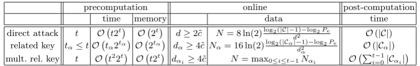
All attacks in this work can be separated in three phases. In theprecomputation phase we compute the correlation for each key, in the online phase we obtain the empirical bias of the plaintext/ciphertext pairs for the secret key and in thepost-computation phase we choose one key-class. A summary of the complexity for the different attacks is given in Table 1. The memory complexity in the multiple related key attack can be reduced to O(2t) if we redo the computation of the key classes separately for each
difference in the post-computation phase. However, this would increase the time complexity of the last phase toO t22t
.
8
Results from Experiments on Reduced Round PRESENT
Table 1.Complexity of the different attacks
precomputation online post-computation
time memory data time
direct attack t O t2t
O 2t
d≥2˜c N= 8 ln(2)log2(|C|−1)−log2Pe
d2 O(|C|)
related key tα≤tO tα2tα
O 2tα
dα≥4˜c Nα= 16 ln(2)log2(
|Cα|−1)−log2Pe d2
α O(|Cα|)
mult. rel. key t O t22t O t2t dαi ≥4˜c N= max0≤i≤t−1Nαi O Pt−1
i=0|Cαi|
of round approximations with an absolute correlation of 2−2. Thus, all strong trails overrrounds have a trail-correlation of absolute value 2−2r. For seven rounds, all strong trails map to separate key-masks,
thus,ρ(v) =±2−14for allv∈ V. We can set ˜c= 2−14 and know thatd≥2−13andd
α≥2−12.
We are using the originalnon-linearkey-schedule of PRESENT. In the 80-bit key case, at every round except for the first one, 4 bits are transformed by an S-box. Thus to construct the target keyK, from which all the round-keys depend in a linear way, we have to extend the original 80-bit key KM by the
bits that are the output from the S-box transformations. For 7 rounds the keyKconsists of`= 104 bits. In the related-key approach we must be careful not to use a difference forK which cannot be achieved by a linear difference inKM.
We only used 1-bit masks for the input and the output, where the output mask is applied directly after the last S-box layer. Letu, w be the bit-position of, respectively, the input and the output mask, then we denote the mask pair by (u, w). The simple structure of the cipher allows to obtain the exact set V includingρ(v) for a given mask quite fast. For example for the 1-bit mask pair (53,37) we could obtainV for 20 rounds in less than 14 seconds.
For our tests, we chose the masks (53,37), fixed a basis and computedα0, . . . , α14. Our choice leads
to the following values:|V= 24|, |C|= 13, t= 15, h= 3.21, hB= 14.25.
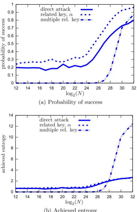
As we have seen, different approaches lead to different amounts of average learned information. To acknowledge this fact, we define the new notion of achieved entropy which is the entropy of a test multiplied by its success probability. Note that we achieve the full entropy hB only if we determine all valuesηi, 0≤i≤t−1, correctly.
In Fig. 1 we consider three different cases: The direckt attack (Section 4), the related key attack for a single difference α (Section 5,|Vα|= 9, |Cα| = 10, tα = 9, hα = 2.63), and the multiple related key
approach (Section 6). In all three cases we give the probability of success and the achieved entropy for 400 random keys and up to N = 232 plaintext/ciphertext pairs. Since the number of keys is not very
high, the graphs still show some uneven behaviour.
We see that the success probability of the single related key attack is always larger than the one for the generic attack. This comes from the fact that|Cα|<|C|, thus we have less choices and a higher
probability to be correct, but also from the fact that dα > d. We only determine the full η correctly if
we determine all the ηi correctly, thus the success probability of the third graph increases later, but in
the end it benefits form the fact thatdαi> d.
When considering the achieved entropy, we see that for some time the single related key approach leads to better results than the direct approach. For N ≥228, the multiple related key approach leads
to the highest achieved entropy.
9
Conclusion
0 0.1 0.2 0.3 0.4 0.5 0.6 0.7 0.8 0.9 1
12 14 16 18 20 22 24 26 28 30 32
(a) Probability of success
0 2 4 6 8 10 12 14
12 14 16 18 20 22 24 26 28 30 32
(b) Achieved entropy
Fig. 1.Empirical results for 400 random keys
The direct attack uses the full value set of the correlation. We have also seen how to reduce this value set by inserting a difference, known to the attacker, in the secret key. This can lead to slightly smaller data complexity and to a reduced time and memory complexity. Similarly, it is possible to consider a related key fault attack by flipping one bit in a known position of the round key. If physically feasible, such an attack would work for any key alternating block cipher and give one bit of information of the round keys provided that the targeted trail correlation is sufficiently large.
We described a way how to exploit a linear hull in Matsui’s Algorithm 1, which has not been analyzed until now. We showed that the data complexity is inversely proportional to the square of the smallest trail correlation. In Algorithm 2 the average data complexity is inversely proportional to the sum of the squares of the trail correlations, which makes the data complexity in general smaller than for Algorithm 1. However, our approach for Algorithm 1 works for all keys and not just for a subset and if the number of trails is small, the difference of the complexity between the two approaches is not very big. As the two algorithms target on different sets of key-bits, Algorithm 1 on the inner round-keys, Algorithm 2 on the external round-keys, Algorithm 1 is not an alternative to Algorithm 2 but typically used in addition to it, which makes these two algorithms not directly comparable.
Acknowledgements
References
1. Baign`eres, T., Vaudenay, S.: The complexity of distinguishing distributions. In: ICITS 2008. pp. 210–222. LNCS, Springer, Heidelberg (2008)
2. Biham, E., Anderson, R., Knudsen, L.: Serpent: A new block cipher proposal. In: Vaudenay, S. (ed.) FSE 1998. LNCS, vol. 1372, pp. 222–238. Springer, Heidelberg (1998)
3. Biryukov, A., Canni`ere, C.D., Quisquater, M.: On Multiple Linear Approximations. In: Franklin, M. (ed.) CRYPTO 2004. LNCS, vol. 3152, pp. 1–22. Springer, Heidelberg (2004)
4. Bogdanov, A., Knudsen, L.R., Leander, G., Paar, C., Poschmann, A., Robshaw, M.J.B., Seurin, Y., Vikkelsoe, C.: PRESENT: An ultra-lightweight block cipher. In: Paillier, P., Verbauwhede, I. (eds.) CHES 2007. LNCS, vol. 4727, pp. 450–466. Springer, Heidelberg (2007)
5. Cover, T.M., Thomas, J.A.: Elements of information theory. Wiley-Interscience, New York, NY, USA (1991) 6. Daemen, J., Govaerts, R., Vandewalle, J.: Correlation matrices. In: Preneel, B. (ed.) FSE 1994. LNCS, vol.
1008, pp. 275–285. Springer, Heidelberg (1995)
7. Daemen, J., Rijmen, V.: The Design of Rijndael: AES - The Advanced Encryption Standard. Springer, Heidelberg (2002)
8. Hermelin, M., Nyberg, K.: Dependent linear approximations - the algorithm of Biryukov and others revisited. In: CT-RSA 2010. LNCS, vol. 5985, pp. 318–333. Springer, Heidelberg (2010)
9. Levy, B.C.: Principles of Signal Detection and Parameter Estimation. Springer, Heidelberg (2008)
10. Matsui, M.: Linear cryptanalysis method for DES cipher. In: Helleseth, T. (ed.) EURORYPT 1993. LNCS, vol. 765, pp. 386–397. Springer, Heidelberg (1994)
11. Murphy, S.: The effectiveness of the linear hull effect. Report RHUL-MA-2009-19, Departmental Technical Report (2009)
12. Nyberg, K.: Linear approximation of block ciphers. In: De Santis, A. (ed.) EUROCRYPT 1994. LNCS, vol. 950, pp. 439–444. Springer, Heidelberg (1995)
13. Nyberg, K.: Correlation theorems in cryptanalysis. Discrete Applied Mathematics 111(1-2), 177–188 (2001) 14. Nyberg, K.: Linear cryptanalysis using multiple linear approximations. Early Symmetric Crypto (ESC 2010) seminar, Remich, Luxembourg, 11-15 January 2010 (2011),https://cryptolux.org/mediawiki.esc/ images/5/52/Esc_nyberg.pdf