A Full Proof of the BGW Protocol for Perfectly-Secure Multiparty Computation

(1)

A Full Proof of the BGW Protocol for Perfectly-Secure

Multiparty Computation

∗

Gilad Asharov† Yehuda Lindell†

January 8, 2018

Abstract

In the setting of secure multiparty computation, a set ofnparties with private inputs wish to jointly compute some functionality of their inputs. One of the most fundamental results of secure computation was presented by Ben-Or, Goldwasser and Wigderson (BGW) in 1988. They demonstrated that any n-party functionality can be computed with perfect security, in the private channels model. When the adversary is semi-honest this holds as long as t < n/2 parties are corrupted, and when the adversary is malicious this holds as long ast < n/3 parties are corrupted. Unfortunately, a full proof of these results was never published. In this paper, we remedy this situation and provide a full proof of security of the BGW protocol. This includes a full description of the protocol for the malicious setting, including the construction of a new subprotocol for the perfect multiplication protocol that seems necessary for the case ofn/4≤t < n/3.

∗

This work was funded by the European Research Council under the European Union’s Seventh Framework Programme (FP/2007-2013) / ERC Grant Agreement n. 239868, and by the _{the israel science foundation} (grant No. 189/11).

†

(2)

1 Introduction

1.1 Background – Secure Computation

In the setting of secure multiparty computation, a set ofnparties with possibly private inputs wish to securely compute some function of their inputs in the presence of adversarial behavior. Loosely speaking, the security requirements from such a computation are that nothing is learned from the protocol other than the output (privacy), that the output is distributed according to the prescribed functionality (correctness), that parties cannot choose their inputs as a function of the others’ inputs (independence of inputs), and that all parties receive output (fairnessandguaranteed output delivery). The actual definition [21, 28, 3,7,19] formalizes this by comparing the result of a real protocol execution with the result of an ideal execution in an ideal model where an incorruptible trusted party carries out the computation for the parties. This definition has come to be known as the “ideal/real simulation paradigm”.

There are many different settings within which secure computation has been considered. Re-garding the adversary, one can consider semi-honest adversaries (who follow the protocol specifi-cation but try to learn more than they should by inspecting the protocol transcript) or malicious adversaries (who may follow an arbitrary strategy). In addition, an adversary may be limited to polynomial-time (as in the computational setting) or unbounded (as in the information-theoretic setting). Finally, the adversary may be static (meaning that the set of corrupted parties is fixed be-fore the protocol execution begins) or adaptive (meaning that the adversary can adaptively choose to corrupt throughout the protocol execution).

Wide reaching feasibility results regarding secure multi-party computation were presented in the mid to late 1980’s. The first feasibility results for secure computation were in the computational setting and were provided by [33] for the two-party case, and by [20] for the multiparty case. These results begged the question as to whether it is possible to avoid computational hardness assumptions; that is, provide analogous results for the information-theoretic setting. This question was answered in the affirmative by [6,13] who showed that when less than a third of the parties are corrupted it is possible to securely compute any functionality in the information-theoretic setting, assuming an ideal private channel between each pair of parties. The protocol of [6] achieved perfect security, while the protocol of [13] achievedstatistical security. These results were followed by [30,2] who showed that if the parties are also given an ideal broadcast channel, then it is possible to securely compute any functionality with statistical security assuming only an honest majority.

1.2 The BGW Protocol

Our focus is on the results of Ben-Or, Goldwasser and Wigderson (BGW) [6], who showed that every functionality can be computed withperfect security in the presence of semi-honest adversaries controlling a minority of parties, and in the presence of malicious adversaries controlling less than a third of the parties. The discovery that secure computation can be carried out information theoretically, and the techniques used by BGW, were highly influential. In addition, as we shall see, the fact that security isperfect – informally meaning that there is azero probability of cheating by the adversary – provides real security advantages over protocols that have a negligible probability of failure (cf. [23]). For this reason, we focus on the BGW protocol [6] rather than on [13].

(4)

computingf. In this computation, the parties compute shares of the output of a circuit gate given shares of the input wires of that gate. To be more exact, the parties first share their inputs with each other using Shamir’s secret sharing [31]; in the case of malicious adversaries, averifiable secret sharing protocol (cf. [14, 20]) is used. The parties then emulate the computation of each gate of the circuit, computing Shamir shares of the gate’s output from the Shamir shares of the gate’s inputs. As we shall see, this secret sharing has the property that addition gates in the circuit can be emulated using local computation only. Thus, the parties only interact in order to emulate the computation of multiplication gates; this step is the most involved part of the protocol. Finally, the parties reconstruct the secrets from the shares of the output wires of the circuit in order to obtain their output.

We proceed to describe the protocol in a bit more detail. Shamir’s secret sharing enables the sharing of a secrets amongst nparties, so that any subset of t+ 1 or more parties can efficiently reconstruct the secret, and any subset of t or less parties learn no information whatsoever about the secret. LetF be a finite field of size greater thann, let α1, . . . , αn ben distinct non-zero field

elements, and lets∈F. Then, in order to shares, a polynomialp(x)∈F[x] of degreetwith constant termsis randomly chosen, and the share of theith partyPi is set top(αi). By interpolation, given

any t+ 1 points it is possible to reconstruct p and compute s = p(0). Furthermore, since p is random, its values at anytor less of theαi’s give no information abouts.

Now, letndenote the number of parties participating in the multiparty computation, and lett be a bound on the number of corrupted parties. The first step of the BGW protocol is for all parties to share their inputs using Shamir’s secret sharing scheme. In the case of semi-honest adversaries, plain Shamir sharing with a threshold t < n/2 is used, and in the case of malicious adversaries verifiable secret sharing (VSS) with a thresholdt < n/3 is used. A verifiable secret sharing protocol is needed for the case of malicious adversaries in order to prevent cheating, and the BGW paper was also the first to construct a perfect VSS protocol.

Next, the parties emulate the computation of the gates of the circuit. The first observation is that addition gates can be computed locally. That is, given sharesp(αi) andq(αi) of the two input

wires to an addition gate, it holds that r(αi) =p(αi) +q(αi) is a valid sharing of the output wire.

This is due to the fact that the polynomial r(x) defined by the sum of the shares has the same degree as both p(x) andq(x), andr(0) =p(0) +q(0).

Regarding multiplication gates, observe that by computing r(αi) = p(αi)·q(αi) the parties

(5)

We remark that t < n/3 is not merely a limitation of the way the BGW protocol works. In particular, the fact that at most t < n/3 corruptions can be tolerated in the malicious model follows immediately from the fact that at most t < n/3 corruptions can be tolerated for Byzantine agreement [29]. In contrast, given a broadcast channel, it is possible to securely compute any functionality with information-theoretic (statistical) security for any t < n/2 [30,2].

1.3 Our Results

Despite the importance of the BGW result, a full proof of its security has never appeared (and this is also the state of affairs regarding [13]). In addition, a full description of the protocol in the malicious setting was also never published. In this paper we remedy this situation and provide a full description and proof of the BGW protocols, for both the semi-honest and malicious settings. We prove security relative to the ideal/real definition of security for multiparty computation. This also involves carefully defining the functionalities and sub-functionalities that are used in order to achieve the result, as needed for presenting a modular proof. Our main result is a proof of the following informally stated theorem:

Theorem 1 (basic security of the BGW protocol – informally stated): Consider a synchronous network with pairwise private channels and a broadcast channel. Then:

1. Semi-honest: For every n-ary functionality f, there exists a protocol for computing f with perfect security in the presence of a static semi-honest adversary controlling up to t < n/2 parties;

2. Malicious: For everyn-ary functionalityf, there exists a protocol for computingf with perfect security in the presence of a static malicious adversary controlling up tot < n/3 parties.

The communication complexity of the protocol is O(poly(n)· |C|) where C is an arithmetic circuit computing f, and the round complexity is linear in the depth of the circuit C.

All of our protocols are presented in a model with pairwise private channelsand secure broad-cast. Since we only consider the case of t < n/3 malicious corruptions, secure broadcast can be achieved in a synchronous network with pairwise channels by running Byzantine Generals [29,

24, 17]. In order to obtain (expected) round complexity linear in the depth of |C|, an expected constant-round Byzantine Generals protocol of [17] (with composition as in [26,5]) is used.

Security under composition. Theorem 1 is proven in the classic setting of a static adversary and stand-alone computation, where the latter means that security is proven for the case that only a single protocol execution takes place at a time. Fortunately, it was shown in [23] that any protocol that isperfectly secure and has a black-box non-rewinding simulator, is also secure under universal composability [8] (meaning that security is guaranteed to hold when many arbitrary protocols are run concurrently with the secure protocol). Since our proof of security satisfies this condition, we obtain the following corollary, which relates to a far more powerful adversarial setting:

(6)

adversary controlling up to t < n/2 parties, and there exists a protocol for computingf with perfect universally composable security in the presence of a static malicious adversary controlling up to t < n/3 parties.

Corollary2refers to information-theoretic security in the ideal private channels model. We now derive a corollary to the computational model with authenticated channels only. In order to derive this corollary, we first observe that information-theoretic security implies security in the presence of polynomial-time adversaries (this holds as long as the simulator is required to run in time that is polynomial in the running time of the adversary, as advocated in [19, Sec. 7.6.1]). Furthermore, the ideal private channels of the information-theoretic setting can be replaced with computationally secure channels that can be constructed over authenticated channels using semantically secure public-key encryption [22,32]. We have:

Corollary 3 (UC computational security of the BGW protocol): Consider a synchronous network with authenticated channels. Assuming the existence of semantically secure public-key encryption, for every n-ary functionalityf there exists a protocol for computingf with universally composable securityin the presence of a static malicious adversary controlling up to t < n/3 parties.

We stress that unlike the UC-secure computational protocols of [12] (that are secure for any t < n), the protocols of Corollary3are in theplain model, with authenticated channels but with no other trusted setup (in particular, no common reference string). Although well accepted folklore, Corollaries 2 and 3 have never been proved. Thus, our work also constitutes the first full proof that universally composable protocols exist in the plain model (with authenticated channels) for any functionality, in the presence of static malicious adversaries controlling anyt < n/3 parties.

Adaptive security with inefficient simulation. In [9] it was shown that any protocol that is proven perfectly secure under the security definition of [15] is also secure in the presence of adaptive adversaries, alas with inefficient simulation. We use this to derive security in the presence of adaptive adversaries, albeit with the weaker guarantee provided by inefficient simulation (in particular, this does not imply adaptive security in the computational setting). See Section 8 for more details.1

Organization. In Section2, we present a brief overview of the standard definitions of perfectly secure multiparty computation and of the modular sequential composition theorem that is used throughout in our proofs. Then, in Section 3, we describe Shamir’s secret sharing scheme and rigorously prove a number of useful properties of this scheme. In Section 4 we present the BGW protocol for the case of semi-honest adversaries. An overview of the overall construction appears in Section4.1, and an overview of the multiplication protocol appears at the beginning of Section4.3. The BGW protocol for the case of malicious adversaries is presented in Sections5to7. In Sec-tion5we present the BGW verifiable secret sharing (VSS) protocol that uses bivariate polynomials. This section includes background on Reed-Solomon encoding and properties of bivariate polyno-mials that are needed for proving the security of the VSS protocol. Next, in Section6 we present the most involved part of the protocol – the multiplication protocol for computing shares of the

1

(7)

product of shares. This involves a number of steps and subprotocols, some of which are new. The main tool for the BGW multiplication protocol is a subprotocol for verifiably sharing the product of a party’s shares. This subprotocol, along with a detailed discussion and overview, is presented in Section 6.6. Our aim has been to prove the security of the original BGW protocol. However, where necessary, some changes were made to the multiplication protocol as described originally in [6]. Finally, in Section7, the final protocol for secure multiparty computation is presented. The protocol is proven secure for any VSS and multiplication protocols that securely realize the VSS and multiplication functionalities that we define in Sections 5 and 6, respectively. In addition, an exact count of the communication complexity of the BGW protocol for malicious adversaries is given. We conclude in Section 8 by showing how to derive security in other settings (adaptive adversaries, composition, and the computational setting).

2 Preliminaries and Definitions

In this section, we review the definition of perfect security in the presence of semi-honest and malicious adversaries. We refer the reader to [19, Sec. 7.6.1] and [7] for more details and discussion. In the definitions below, we consider the stand-alone setting with a synchronous network, and perfectly private channels between all parties. For simplicity, we will also assume that the parties have a broadcast channel; as is standard, this can be implemented using an appropriate Byzantine Generals protocol [29, 24]. Since we consider synchronous channels and the computation takes place in clearly defined rounds, if a message is not received in a given round, then this fact is immediately known to the party who is supposed to receive the message. Thus, we can write “if a message is not received” or “if the adversary does not send a message” and this is well defined. We consider static corruptions meaning that the set of corrupted parties is fixed ahead of time, and the stand-alone setting meaning that only a single protocol execution takes place; extensions to the case of adaptive corruptions and composition are considered in Section8.

Basic notation. For a set A, we writea∈_R A when a is chosen uniformly from A. We denote the number of parties by n, and a bound on the number of corrupted parties by t. Let f : ({0,1}∗)n→({0,1}∗)nbe a possibly probabilisticn-ary functionality, wherefi(x1, . . . , xn) denotes

the ith element of f(x1, . . . , xn). We denote by I ={i1, . . . i`} ⊂[n] the indices of the corrupted

parties, where [n] denotes the set {1, . . . , n}. By the above, |I| ≤t. Let ~x = (x1, . . . , xn), and let ~

xI and fI(~x) denote projections of the correspondingn-ary sequence on the coordinates in I; that

is, ~xI = (xi1, . . . , xi`) and fI(x~) = (fi1(~x), . . . , fi`(~x)). Finally, to ease the notation, we omit the

indexi when we write the set {(i, ai)}in=1 and simply write {ai}ni=1. Thus, for instance, the set of shares{(i1, f(αi1)), . . . ,(i`, f(αi`))} is denoted as{f(αi)}i∈I.

Terminology. In this paper, we consider security in the presence of both semi-honest and mali-cious adversaries. As in [19], we call security in the presence of a semi-honest adversary controlling t parties t-privacy, and security in the presence of a malicious adversary controlling t parties t

(8)

2.1 Perfect Security in the Presence of Semi-Honest Adversaries

We are now ready to define security in the presence of semi-honest adversaries. Loosely speaking, the definition states that a protocol is t-private if the view of up to t corrupted parties in a real protocol execution can be generated by a simulator given only the corrupted parties’ inputs and outputs.

Theviewof theith partyPi during an execution of a protocolπ on inputs~x, denotedviewπi(~x),

is defined to be (xi, ri;mi1, . . . , mik) wherexi isPi’s private input,ri is its internal coin tosses, and

mij is thejth message that was received byPi in the protocol execution. For everyI ={i1, . . . i`},

we denoteviewπI(~x) = (viewπi1(x~), . . .viewπi`(~x)). Theoutputof all parties from an execution of π

on inputs ~x is denotedoutputπ(~x); observe that the output of each party can be computed from

its own (private) view of the execution.

We first present the definition for deterministic functionalities, since this is simpler than the general case of probabilistic functionalities.

Definition 2.1 (t-privacy ofn-party protocols – deterministic functionalities): Letf : ({0,1}∗)n→

({0,1}∗)n be a deterministic n-ary functionality and let π be a protocol. We say thatπ is t-private for f if for every ~x∈({0,1}∗)n _where _|_x

1|=. . .=|xn|,

outputπ(x1, . . . , xn) =f(x1, . . . , xn) (2.1)

and there exists a probabilistic polynomial-time algorithmS such that for everyI ⊂[n]of cardinality at mostt, and every ~x∈({0,1}∗)n where |x1|=. . .=|xn|, it holds that:

n

S(I, ~xI, fI(~x)) o

≡n_viewπ_I(~x)o (2.2)

The above definition separately considers the issue of output correctness (Eq. (2.1)) and privacy (Eq. (2.2)), where the latter captures privacy since the ability to generate the corrupted parties’ view given only the input and output means that nothing more than the input and output is learned from the protocol execution. However, in the case of probabilistic functionalities, it is necessary to intertwine the requirements of privacy and correctness and consider the joint distribution of the output ofS and of the parties; see [7,19] for discussion. Thus, in the general case of probabilistic functionalities, the following definition oft-privacy is used.

Definition 2.2 (t-privacy of n-party protocols – general case): Let f : ({0,1}∗)n →({0,1}∗)n be a probabilistic n-ary functionality and let π be a protocol. We say that π is t-private for f if there exists a probabilistic polynomial-time algorithmS such that for everyI ⊂[n]of cardinality at most t, and every ~x∈({0,1}∗)n where |x1|=. . .=|xn|, it holds that:

n

(S(I, ~xI, fI(~x)), f(~x)) o

≡n(viewπI(x~),outputπ(~x)) o

. (2.3)

(9)

Our presentation – deterministic functionalities. For the sake of simplicity and clarity, we present the BGW protocol and prove its security for the case of deterministic functionalities only. This enables us to prove the overall BGW protocol using Definition 2.1, which makes the proof significantly simpler. Fortunately, this does not limit our result since it has already been shown that it is possible tot-privately computeany probabilistic functionality using a general protocol for t-privately computing any deterministic functionality; see [19, Sec. 7.3.1].

2.2 Perfect Security in the Presence of Malicious Adversaries

We now consider malicious adversaries that can follow an arbitrary strategy in order to carry out their attack; we stress that the adversary is not required to be efficient in any way. Security is formalized by comparing a real protocol execution to an ideal model where the parties just send their inputs to the trusted party and receive back outputs. See [7,19] for details on how to define these real and ideal executions; we briefly describe them here.

Real model: In the real model, the parties run the protocol π. We consider a synchronous network with private point-to-point channels, and an authenticated broadcast channel. This means that the computation proceeds in rounds, and in each round parties can send private messages to other parties and can broadcast a message to all other parties. We stress that the adversary cannot read or modify messages sent over the point-to-point channels, and that the broadcast channel is authenticated, meaning that all parties know who sent the message and the adversary cannot tamper with it in any way. Nevertheless, the adversary is assumed to be rushing, meaning that in every given round it can see the messages sent by the honest parties before it determines the messages sent by the corrupted parties.

Let π be a n-party protocol, let A be an arbitrary machine with auxiliary input z, and let I ⊂[n] be the set of corrupted parties controlled by A. We denote byREAL_π,_A(_z₎_,I(~x) the random variable consisting of the view of the adversary Aand the outputs of the honest parties, following a real execution ofπ in the aforementioned real model, where for everyi∈[n], party Pi has input xi.

Ideal model: In the ideal model for a functionality f, the parties send their inputs to an incor-ruptible trusted party who computes the output for them. We denote the ideal adversary by S

(since it is a “simulator”), and the set of corrupted parties byI. An execution in the ideal model works as follows:

• Input stage: The adversaryS for the ideal model receives auxiliary inputzand sees the inputs xi of the corrupted parties Pi (for alli∈I ). S can substitute any xi with any x0i of its choice

under the condition that |x0_i|=|xi|.

• Computation: Each party sends its (possibly modified) input to the trusted party; denote the inputs sent by x0₁, . . . , x0_n. The trusted party computes (y1, . . . , yn) = f(x01, . . . , x0n) and sends yj toPj, for everyj∈[n].

• Outputs: Each honest party Pj (j /∈I) outputs yj, the corrupted parties output ⊥, and the

adversary S outputs an arbitrary function of its view.

(10)

shorthand for saying that the input is sent to the trusted party who computes the functionality. We denote by IDEALf,S(z),I(~x) the outputs of the ideal adversary S controlling the corrupted

parties in I and of the honest parties after an ideal execution with a trusted party computing f, upon inputsx1, . . . , xnfor the parties and auxiliary inputzforS. We stress that the communication

between the trusted party andP1, . . . , Pn is over an ideal private channel.

Definition of security. Informally, we say that a protocol is secure if its real-world behavior can be emulated in the ideal model. That is, we require that for every real-model adversary A there exists an ideal-model adversarySsuch that the result of a real execution of the protocol withAhas the same distribution as the result of an ideal execution with S. This means that the adversarial capabilities ofA in a real protocol execution are just whatS can do in the ideal model.

In the definition of security, we require that the ideal-model adversarySrun in time that is poly-nomial in the running time ofA, whatever the latter may be. As argued in [7,19] this definitional choice is important since it guarantees that information-theoretic security implies computational security. In such a case, we say thatS is ofcomparable complexity toA.

Definition 2.3 Let f : ({0,1}∗)n → ({0,1}∗)n be an n-ary functionality and let π be a protocol. We say that π ist-secure for f if for every probabilistic adversaryA in the real model, there exists a probabilistic adversary S of comparable complexity in the ideal model, such that for everyI ⊂[n] of cardinality at mostt, every~x∈({0,1}∗₎n _where _|_x

1|=. . .=|xn|, and everyz∈ {0,1}∗, it holds that:

n

IDEALf,S(z),I(~x) o

≡nREAL_π,_A(_z₎_,I(~x) o

.

Reactive functionalities. The above definition refers to functionalities that map inputs to out-puts in a single computation. However, some computations take place in stages, and state is preserved between stages. Two examples of such functionalities are mental poker (where cards are dealt and thrown and redealt [20]) and commitment schemes (where there is a separate commit-ment and decommitcommit-ment phase; see [8] for a definition of commitments via an ideal functionality). Such functionalities are calledreactive, and the definition of security is extended to this case in the straightforward way by allowing the trusted party to obtain inputs and send outputs in phases; see [19, Section 7.7.1.3].

2.3 Modular Composition

The sequential modular composition theorem [7] is an important tool for analyzing the security of a protocol in a modular way. Letπf be a protocol for securely computingf that uses a subprotocol πg for computing g. Then, the theorem states that it suffices to consider the execution of πf in

a hybrid model where a trusted third party is used to ideally compute g (instead of the parties running the real subprotocol πg). This theorem facilitates a modular analysis of security via the

following methodology: First prove the security ofπg, and then prove the security ofπf in a model

allowing an ideal party for g. The model in which πf is analyzed using ideal calls to g, instead of

executingπg, is called theg-hybrid modelbecause it involves both a real protocol execution and an

ideal trusted third party computingg.

(11)

run the subprotocolπg using inputsu1, . . . , un, then each partyPi simply writesui to its outgoing

oracle tape. Then, in the next round, it receives back the output gi(u1, . . . , un) on its incoming

oracle tape. We denote byHYBRIDg_π

f,A(z),I(~x) an execution of protocol πf where each call to πg is

carried out using an oracle computingg. See [7, 19] for a formal definition of this model for both the semi-honest and malicious cases, and for proofs that ifπf is t-private (resp., t-secure) forf in

theg-hybrid model, andπg ist-private (resp., t-secure) forg, thenπf when run in the real model

using πg ist-private (resp., t-secure) forf.

3 Shamir’s Secret Sharing Scheme [

31 ] and Its Properties

3.1 The Basic Scheme

A central tool in the BGW protocol is Shamir’s secret-sharing scheme [31]. Roughly speaking, a (t+ 1)-out-of-n secret sharing scheme takes as input a secrets from some domain, and outputsn shares, with the property that it is possible to efficiently reconstruct s from every subset oft+ 1 shares, but every subset of t or less shares reveals nothing about the secret s. The value t+ 1 is called thethresholdof the scheme. Note that in the context of secure multiparty computation with up to t corrupted parties, the threshold of t+ 1 ensures that the corrupted parties (even when combining allt of their shares) can learn nothing.

A secret sharing scheme consist of two algorithm: the first algorithm, called thesharing algorithm, takes as input the secret s and the parameters t+ 1 and n, and outputs n shares. The second algorithm, called the reconstruction algorithm, takes as input t+ 1 or more shares and outputs a value s. It is required that the reconstruction of shares generated from a values yields the same values.

Informally, Shamir’s secret-sharing scheme works as follows. LetFbe a finite field of size greater thannand lets∈_F. The sharing algorithm defines a polynomialq(x) of degreetinF[x], such that its constant term is the secret s and all the other coefficients are selected uniformly and indepen-dently at random in F.2 Finally, the shares are defined to be q(αi) for every i∈ {1, . . . , n}, where α1, . . . , αn are anyndistinct non-zero predetermined values inF. The reconstruction algorithm of this scheme is based on the fact that any t+ 1 points define exactly one polynomial of degree t. Therefore, using interpolation it is possible to efficiently reconstruct the polynomialq(x) given any subset of t+ 1 points (αi, q(αi)) output by the sharing algorithm. Finally, givenq(x) it is possible

to simply computes=q(0). We will actually refer to reconstruction using allnpoints, even though t+ 1 suffice, since this is the way that we use reconstruction throughout the paper.

In order to see that any subset oftor less shares reveals nothing abouts, observe that for every set of t points (αi, q(αi)) and every possible secret s0 ∈F, there exists a unique polynomial q0(x) such that q0(0) = s0 and q0(αi) = q(αi). Since the polynomial is chosen randomly by the sharing

algorithm, there is the same likelihood that the underlying polynomial isq(x) (and so the secret is s) and that the polynomial isq0(x) (and so the secret iss0). We now formally describe the scheme.

Shamir’s (t+ 1)-out-of-n secret sharing scheme. Let F be a finite field of order greater thann, letα1, . . . , αn be any distinct non-zero elements of F, and denote~α= (α1, . . . , αn). For a

polynomial q Leteval~α(q(x)) = (q(α1), . . . , q(αn)). 2

(12)

• The sharing algorithm forα1, . . . , αn: Letshare~α(s, t+1) be the algorithm that receives for

inputsandt+ 1 wheres∈_Fandt < n. Then,shareα~ choosestrandom valuesq1, . . . qt∈RF, independently and uniformly distributed inF, and defines the polynomial:

q(x) =s+q1x+. . . qtxt

where all calculations are in the fieldF. Finally,share~αoutputsevalα~(q(x)) = (q(α1), . . . , q(αn)),

whereq(αi) is the share of party Pi.

• The reconstruction algorithm: Algorithmreconstructα~(β1, . . . , βn) finds the unique

poly-nomial q(x) of degree t such that for every i= 1, . . . , n it holds that q(αi) =βi, when such

a polynomial exists (this holds as long as β1, . . . , βn all lie on a single polynomial). The

algorithm then outputs the coefficients of the polynomial q(x) (note that the original secret can be obtained by simply computings=q(0)).

By the above notation, observe that for every polynomial q(x) of degree t < n, it holds that

reconstruct~α(eval~α(q(x))) =q(x). (3.1)

Notation. LetPs,t_{be the set of all polynomials with degree less than or equal to}_t_{with constant}

terms. Observe that for every two valuess, s0 ∈F, it holds that|Ps,t_|₌_|Ps0,t_|₌_|

F|t.

3.2 Basic Properties

In this section, we prove some basic properties of Shamir’s secret sharing scheme (the proofs of these claims are standard but appear here for the sake of completeness). We first show that the value of a polynomial chosen at random from Ps,t _{at any single non-zero point is distributed uniformly at}

random inF; this can be generalized to hold for anyt points.

Claim 3.1 For every t≥1, and for every s, α, y∈Fwith α6= 0, it holds that:

Pr

q∈RPs,t

[q(α) =y] = 1

|_F|.

Proof: Fix s, y and α with α = 0. Denote the6 ith coefficient of the polynomial q(x) by qi, for i= 1, . . . , t. Then:

Pr [q(α) =y] = Pr

"

y =s+

t X

i=1 qiαi

#

= Pr

"

y=s+q1α+

t X

i=2 qiαi

#

where the probability is taken over the random choice ofq ∈RPs,t, or equivalently of the coefficients q1, . . . , qt∈RF. Fixq2, . . . , qtand denote v=Pt_i₌₂qiαi. Then, for a randomly chosen q1 ∈RFwe have that

Pr

h

q(α) =y i

= Pr

h

y=s+q1α+v

i

= Prhq1α=y−s−v

i

= Prhq1 =α−1·(y−s−v)

i

= 1

(13)

where the third equality holds since α∈_Fand α6= 0 implying thatα has an inverse, and the last equality is due to the fact that q1∈RF is randomly chosen.

In the protocol for secure computation, a dealer hides a secret sby choosing a polynomialf(x) at random from Ps,t_{, and each party} _P

i receives a share, which is a point f(αi). In this context,

the adversary controls a subset of at most t parties, and thus receives at most t shares. We now show that any subset of at most t shares does not reveal any information about the secret. In Section3.1, we explained intuitively why the above holds. This is formalized in the following claim that states that for every subset I ⊂ [n] with |I| ≤ t and every two secrets s, s0, the distribution over the shares seen by the parties Pi (i∈I) when sis shared is identical to whens0 is shared.

Claim 3.2 For any set of distinct non-zero elements α1, . . . , αn∈F, any pair of values s, s0 ∈F, any subset I ⊂[n]where |I|=`≤t, and every ~y∈_F` _{it holds that:}

Pr

f(x)∈RPs,t

h ~

y = {f(αi)}_i∈I i

= Pr

g(x)∈RPs

0_,t h

~

y= {g(αi)}_i∈I i

= 1

|_F|`

where f(x) and g(x) are chosen uniformly and independently from Ps,t _and_Ps0,t_{, respectively.}

Proof: We first prove the claim for the special case that`=t. Fix s, s0 ∈_F, fix non-zero elements α1, . . . , αn ∈F, and fixI ⊂[n] with |I|=t. Moreover, fix ~y ∈Ft. Letyi be theith element of the

vector~y for everyi∈ {1, . . . , t}. We now show that:

Pr

f(x)∈RPs,t

h ~

y= {f(αi)}_i∈I i

= 1

|Ps,t_|.

The values of ~y define a unique polynomial from Ps,t_{. This is because there exists a single}

polynomial of degree t that passes through the points (0, s) and {(αi, yi)}i∈I. Let f0(x) be this

unique polynomial. By definition we have that f0(x)∈ Ps,t _{and so:}

Pr

f(x)∈RPs,t

h

~y= {f(αi)}i∈I i

= Pr

f(x) =f0(x)

= 1

|Ps,t_|

where the latter is true since f(x) is chosen uniformly at random from Ps,t_{, and} _f0₍_x_{) is a fixed} polynomial in Ps,t_.

Using the same reasoning, and letting g0(x) be the unique polynomial that passes through the points (0, s0) and{(αi, yi)}i∈I we have that:

Pr

g(x)∈RPs

0_,t h

~

y= {g(αi)}_i∈I i

= Prg(x) =g0(x)= 1

|Ps0_,t

|.

The proof for the case of `=t is concluded by observing that for everysands0 inF, it holds that

|Ps,t_|₌_|Ps0_,t

|=|_F|t_{, and so:}

Pr

f(x)∈RPs,t

h

~y= {f(αi)}i∈I i

= Pr

g(x)∈RPs0,t

h ~

y= {g(αi)}i∈I i

= 1

|F|t.

For the general case where |I|=` may be less thant, fixJ ⊂[n] with|J|=tand I ⊂J. Observe that for every vector ~y∈F`:

Pr

f(x)∈RPs,t

h ~

y= {f(αi)}_i∈I i

= X

~ y0_∈

Ft−`

Pr

h

(~y, ~y0) =

{f(αi)}_i∈I,{f(αj)}j∈J\I i

=|F|t−`· 1

|_F|t =

1

(14)

This holds for both sand s0 and so the proof is concluded.

As a corollary, we have that any`≤tpoints on a random polynomial are uniformly distributed in the field F. This follows immediately from Claim3.2 because stating that every~y appears with probability 1/|_F|` _{is equivalent to stating that the shares are uniformly distributed. That is:}

Corollary 3.3 For any secret s ∈ _F, any set of distinct non-zero elements α1, . . . , αn ∈ F, and any subset I ⊂[n]where |I|=`≤t, it holds that n{f(αi)}i∈I

o

≡nU(1) F , . . . , U

(`)

F o

, where f(x) is chosen uniformly at random from Ps,t _and _U(1)

F , . . . , U

(`)

F are ` independent random variables that are uniformly distributed over F.

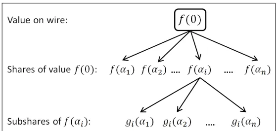
Multiple polynomials. In the protocol for secure computation, parties hide secrets and dis-tribute them using Shamir’s secret sharing scheme. As a result, the adversary receives m · |I|

shares, {f1(αi), . . . , fm(αi)}i∈I, for some value m. The secrets f1(0), . . . , fm(0) may not be

inde-pendent. We therefore need to show that the shares that the adversary receives for all secrets do not reveal any information about any of the secrets. Intuitively, this follows from the fact that Claim 3.2is stated for any two secrets s, s0, and in particular for two secrets that are known and may be related. The following claim can be proven using standard facts from probability:

Claim 3.4 For any m ∈ N, any set of non-zero distinct values α1, . . . , αn ∈ F, any two sets of secrets (a1, . . . , am) ∈ Fm and (b1, . . . , bm) ∈ Fm, and any subset I ⊂ [n] of size |I| ≤ t, it holds that:

n

{(f1(αi), . . . , fm(αi))}i∈I o

≡n{(g1(αi), . . . , gm(αi))}i∈I o

where for every j, fj(x), gj(x) are chosen uniformly at random from Paj,t and Pbj,t, respectively.

Hiding the leading coefficient. In Shamir’s secret sharing scheme, the dealer creates shares by constructing a polynomial of degreet, where its constant term is fixed and all the other coefficients are chosen uniformly at random. In Claim 3.2 we showed that any t or fewer points on such a polynomial do not reveal any information about the fixed coefficient which is the constant term.

We now consider this claim when we choose the polynomial differently. In particular, we now fix the leading coefficient of the polynomial (i.e., the coefficient of the monomial xt), and choose all the other coefficients uniformly and independently at random, including the constant term. As in the previous section, it holds that any subset oft or fewer points on such a polynomial do not reveal any information about the fixed coefficient, which in this case is the leading coefficient. We will need this claim for proving the security of one of the sub-protocols for the malicious case (in Section6.6).

Let Plead

s,t be the set of all the polynomials of degree t with leading coefficient s. Namely, the

polynomials have the structure: f(x) =a0+a1x+. . . at−1xt−1+sxt. The following claim is derived similarly to Corollary3.3.

Claim 3.5 For any secret s ∈ _F, any set of distinct non-zero elements α1, . . . , αn ∈ F, and any subset I ⊂[n] where |I|=`≤t, it holds that:

n

{f(αi)}_i∈I o

≡nU(1) F , . . . , U

(`)

F o

where f(x) is chosen uniformly at random from Plead s,t andU

(1)

F , . . . , U

(`)

(15)

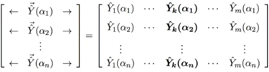
3.3 Matrix Representation

In this section we present a useful representation for polynomial evaluation. We being by defining the Vandermonde matrix for the valuesα1, . . . , αn. As is well known, the evaluation of a polynomial

atα1, . . . , αn can be obtained by multiplying the associated Vandermonde matrix with the vector

containing the polynomial coefficients.

Definition 3.6 (Vandermonde matrix for (α1, . . . , αn)): Let α1, . . . , αn be n distinct non-zero el-ements inF. The Vandermonde matrix Vα~ for ~α= (α1, . . . , αn) is the n×n matrix overF defined by V~α[i, j]

def

= (αi)j−1. That is,

V~α

def =          

1 α1 . . . (α1)n−1 1 α2 . . . (α2)n−1

..

. ... ...

1 αn . . . (αn)n−1           (3.2)

The following fact from linear algebra will be of importance to us:

Fact 3.7 Let ~α= (α1, . . . , αn), where allαi are distinct and non-zero. Then,V~α is invertible.

Matrix representation of polynomial evaluations. Let Vα~ be the Vandermonde matrix for ~

α and letq=q0+q1x+· · ·+qtxt be a polynomial wheret < n. Define the vector~q of lengthnas

follows: ~q def= (q0, . . . qt,0, . . . ,0). Then, it holds that:

V~α·~q =          

1 α1 . . . (α1)n−1 1 α2 . . . (α2)n−1

..

. ... ...

1 αn . . . (αn)n−1           ·           q0 .. . qt 0 .. . 0           =          

q(α1)

.. .

q(αn)          

which is the evaluation of the polynomialq(x) on the points α1, . . . , αn.

4 The Protocol for Semi-Honest Adversaries

4.1 Overview

(16)

assume that the arithmetic circuitC consists of three types of gates: addition gates, multiplication gates, andmultiplication-by-a-constant gates. Recall that since a circuit is acyclic, it is possible to sort the wires so that for every gate the input wires come before the output wires.

The protocol works by having the parties jointly propagate values through the circuit from the input wires to the output wires, so that at each stage of the computation the parties obtain Shamir shares of the value on the wire that is currently being computed. In more detail, the protocol has three phases:

• The input sharing stage: In this stage, each party creates shares of its input using Shamir’s secret sharing scheme using threshold t+ 1 (for a given t < n/2), and distributes the shares among the parties.

• The circuit emulation stage: In this stage, the parties jointly emulate the computation of the circuitC, gate by gate. In each step, the parties compute shares of the output of a given gate, based on the shares of the inputs to that gate that they already have. The actions of the parties in this stage depends on the type of gate being computed:

1. Addition gate: Given shares of the input wires to the gate, the output is computed without any interaction by each party simply adding their local shares together. Let the inputs to the gate be a and b and let the shares of the parties be defined by two degree-t polynomials fa(x) and fb(x) (meaning that each party Pi holds fa(αi) and fb(αi) where fa(0) =a and fb(0) =b). Then the polynomial fa+b(x) defined by shares fa+b(αi) =fa(αi) +fb(αi), for everyi, is a degree-tpolynomial with constant terma+b.

Thus, each party simply locally adds its own sharesfa(αi) andfb(αi) together, and the

result is that the parties hold legal shares of the sum of the inputs, as required.

2. Multiplication-by-a-constant gate: This type of gate can also be computed without any interaction. Let the input to the gate be a and let fa(x) be the t-degree polynomial

defining the shares, as above. The aim of the parties is to obtain shares of the valuec·a, wherecis the constant of the gate. Then, each partyPi holdingfa(αi) simply defines its

output share to be fc·a(αi) =c·fa(αi). It is clear thatfc·a(x) is a degree-t polynomial

with constant termc·a, as required.

3. Multiplication gate: As in (1) above, let the inputs beaandb, and letfa(x) andfb(x) be

the polynomials defining the shares. Here, as in the case of an addition gate, the parties can just multiply their shares together and define h(αi) =fa(αi)·fb(αi). The constant

term of this polynomial isa·b, as required. However,h(x) will be of degree 2tinstead of t; after repeated multiplications the degree will benor greater and the parties’nshares will not determine the polynomial or enable reconstruction. In addition,h(x) generated in this way is not a “random polynomial” but has a specific structure. For example,h(x) is typically not irreducible (since it can be expressed as the product offa(x) andfb(x)),

and this may leak information. Thus, local computation does not suffice for computing a multiplication gate. Instead, the parties compute this gate by running an interactive protocol that t-privately computes the multiplication functionality Fmult, defined by

Fmult

(fa(α1), fb(α1)), . . . ,(fa(αn), fb(αn))

=

fab(α1), . . . , fab(αn)

(4.1)

wherefab(x)∈RPa·b,tis a random degree-t polynomial with constant terma·b.3 3

(17)

• The output reconstruction stage: At the end of the computation stage, the parties hold shares of the output wires. In order to obtain the actual output, the parties send their shares to one another and reconstruct the values of the output wires. Specifically, if a given output wire defines output for party Pi, then all parties send their shares of that wire value to Pi.

Organization of this section. In Section4.2, we fully describe the above protocol and prove its security in theFmult-hybrid model. (Recall that in this model, the parties have access to a trusted

party who computes Fmult for them, and in addition exchange real protocol messages.) We also

derive a corollary fort-privately computing any linear function in the plain model (i.e., without any use of the Fmult functionality), that is used later in Section 4.3.3. Then, in Section4.3, we show

how to t-privately compute the Fmult functionality for anyt < n/2. This involves specifying and

implementing two functionalitiesF_rand2t andF_reducedeg ; see the beginning of Section4.3for an overview of the protocol fort-privately computing Fmult and for the definition of these functionalities.

4.2 Private Computation in the Fmult-Hybrid Model

In this section we present a formal description and proof of the protocol fort-privately computing any deterministic functionalityf in theFmult-hybrid model. As we have mentioned, it is assumed

that each party has a single input in a known fieldFof size greater thann, and that the arithmetic circuitC is over F. See Protocol4.1for the description.

We now prove the security of Protocol 4.1. We remark that in the Fmult-hybrid model, the

protocol is actuallyt-private foranyt < n. However, as we will see, in order tot-privately compute theFmult functionality, we will need to set t < n/2.

Theorem 4.2 LetFbe a finite field, letf :Fn→Fnbe ann-ary functionality, and lett < n. Then, Protocol 4.1 is t-private for f in the Fmult-hybrid model, in the presence of a static semi-honest adversary.

Proof: Intuitively, the protocol is t-private because the only values that the parties see until the output stage are random shares. Since the threshold of the secret sharing scheme used is t+ 1, it holds that no adversary controlling t parties can learn anything. The fact that the view of the adversary can be simulated is due to the fact thattshares of any two possible secrets are identically distributed; see Claim 3.2. This implies that the simulator can generate the shares based on any arbitrary value, and the resulting view is identical to that of a real execution. Observe that this is true until the output stage where the simulator must make the random shares that were used match the actual output of the corrupted parties. This is not a problem because, by interpolation, any set of t shares can be used to define a t-degree polynomial with its constant term being the actual output.

SinceCcomputes the functionalityf, it is immediate thatoutputπ(x1, . . . , xn) =f(x1, . . . , xn),

whereπ denotes Protocol4.1. We now proceed to show the existence of a simulator S as required by Definition 2.1. Before describing the simulator, we present some necessary notation. Our proof works by inductively showing that the partial view of the adversary at every stage is identical in the simulated and real executions. Recall that the view of partyPiis the vector (xi, ri;m1i, . . . , m`i),

where xi is the party’s input, ri its random tape, mki is the kth message that it receives in the

(18)

PROTOCOL 4.1 (t-Private Computation in the Fmult-Hybrid Model)

• Inputs: Each partyPi has an input xi∈F.

• Auxiliary input: Each party Pi has an arithmetic circuit C over the fieldF, such that for every~x∈Fn it holds that C(~x) =f(~x), wheref : Fn →Fn. The parties also have a description ofFand distinct non-zero values α1, . . . , αn inF.

• The protocol:

1. The input sharing stage: Each party Pi chooses a polynomial qi(x) uniformly from the set Pxi,t _{of all polynomials of degree} _t _{with constant term} _x

i. For every

j∈ {1, . . . , n},Pi sends partyPj the valueqi(αj).

Each partyPi records the valuesq1(αi), . . . , qn(αi) that it received.

2. The circuit emulation stage: LetG1, . . . , G` be a predetermined topological or-dering of the gates of the circuit. Fork= 1, . . . , `the parties work as follows:

– Case 1 – Gk is an addition gate: Letβki andγki be the shares of input wires held by partyPi. Then,Pi defines its share of the output wire to beδki =β

k i +γ

k i. – Case 2 –Gk is a multiplication-by-a-constant gate with constantc: Letβikbe the

share of the input wire held by partyPi. Then,Pidefines its share of the output wire to beδ_ik=c·βk_i.

– Case 3 –Gk is a multiplication gate: Letβik andγik be the shares of input wires held by party Pi. Then, Pi sends (βik, γik) to the ideal functionality Fmult of Eq. (4.1) and receives back a valueδk

i. PartyPi defines its share of the output wire to beδk

i.

3. The output reconstruction stage: Leto1, . . . , onbe the output wires, where party

Pi’s output is the value on wireoi. For every k= 1, . . . , n, denote byβk1, . . . , βnk the shares that the parties hold for wireok. Then, eachPi sendsPk the shareβki. Upon receiving all shares,Pk computesreconstruct~α(β1k, . . . , βkn) and obtains a poly-nomialgk(x) (note thatt+ 1 of thenshares suffice). Pk then defines its output to be

gk(0).

execution, and` is the overall number of messages received (in our context here, we let mk_i equal the series of messages thatPi receives when the parties compute gate Gk). For the sake of clarity,

we add to the view of each party the values σ1

i, . . . , σ`i, where σik equals the shares on the wires

that Party Pi holds after the parties emulate the computation of gateGk. That is, we denote

viewπi(~x) =

xi, ri;m1i, σi1, . . . , m`i, σi`

.

We stress that since theσk

i values can be efficiently computed from the party’s input, random tape

and incoming messages, the view including the σk_i values is equivalent to the view without them, and this is only a matter of notation.

We are now ready to describe the simulator S. Loosely speaking, S works by simply sending random shares of arbitrary values until the output stage. Then, in the final output stage S sends values so that the reconstruction of the shares on the output wires yield the actual output.

(19)

• Input: The simulator receives the inputs and outputs, {xi}i∈I and {yi}i∈I respectively, of all corrupted parties.

• Simulation:

1. Simulating the input sharing stage:

(a) For everyi∈I, the simulatorS chooses a uniformly distributed random tape forPi; this random tape and the input xi fully determines the degree-t polynomial q0i(x) ∈ Pxi,t _{chosen by} _P

i in the protocol.

(b) For everyj /∈I, the simulatorS chooses a random degree-tpolynomialq0_k(x)∈_RP0,t with constant term 0.

(c) The view of the corrupted party Pi in this stage is then constructed by S to be the set of values{qj(αi)}j /∈I (i.e., the share sent by each honest Pj to Pi). The view of the adversaryA consists of the view of Pi for everyi∈I.

2. Simulating the circuit emulation stage: For every Gk∈ {G1, . . . , G`}:

(a) Gk is an addition gate: Let {fa(αi)}i∈I and {fb(αi)}i∈I be the shares of the input wires of the corrupted parties that were generated by S (initially these are input wires and so the shares are defined byq0_k(x) above). For every i∈I, the simulator

S computes fa(αi) +fb(αi) = (fa+fb)(αi) which defines the shares of the output wire ofGk.

(b) Gk is a multiplication-with-constant gate: Let {fa(αi)}i∈I be the shares of the input wire and let c ∈_F be the constant of the gate. S computes c·fa(αi) = (c·fa)(αi) for everyi∈I which defines the shares of the output wire of Gk.

(c) Gk is a multiplication gate: S chooses a degree-t polynomial fab(x) uniformly at random from P0,t _{(irrespective of the shares of the input wires), and defines the} shares of the corrupted parties of the output wire ofGk to be{fab(αi)}i∈I.

S adds the shares to the corrupted parties’ views.

3. Simulating the output reconstruction stage: Let o1, . . . , on be the output wires. We now focus on the output wires of the corrupted parties. For every k ∈ I, the simulator S

has already defined |I| shares{β_ki}_i∈I for the output wireok. S thus chooses a random

polynomial g0_k(x) of degree t under the following constraints:

(a) g_k0(0) =yk, where yk is the corruptedPk’s output (the polynomial’s constant term is the correct output).

(b) For every i∈I, g0_k(αi) =β_ki (i.e., the polynomial is consistent with the shares that have already been defined).

(Note that if|I|=t, then the above constraints yieldt+ 1equations, which in turn fully determine the polynomial g0_k(x). However, if |I|< t, then S can carry out the above by choosing t− |I|additional random points and interpolating.)

Finally, S adds the shares {g0_k(α1), . . . , g0k(αn)} to the view of the corrupted partyPk. 4. S outputs the views of the corrupted parties and halts.

Denote by view]πI(~x) the viewof the corrupted parties up to the output reconstruction stage

(and not including that stage). Likewise, we denote by ˜S(I, ~xI, fI(~x)) the view generated by the

(20)

We begin by showing that the partial views of the corrupted parties up to the output recon-struction stage in the real execution and simulation are identically distributed.

Claim 4.3 For every ~x∈_Fn _{and every} _I _⊂_[_n_]_with _|_I_{| ≤}_t, n

]

viewπI(~x) o

≡nS˜(I, ~xI, fI(~x)) o

Proof: The only difference between the partial views of the corrupted parties in a real and simulated execution is that the simulator generates the shares in the input-sharing stage and in multiplication gates from random polynomials with constant term 0, instead of with the correct value defined by the actual inputs and circuit. Intuitively, the distributions generated are the same since the shares are distributed identically, for every possible secret.

Formally, we construct an algorithmHthat receives as inputn−|I|+`sets of shares: n−|I|sets of shares{(i, β_i1)}i∈I, . . . ,{(i, βn

−|I|

i )}i∈I and`sets of shares{(i, γi1)}i∈I, . . . ,{(i, γi`)}i∈I. Algorithm H generates the partial view of the corrupted parties (up until but not including the output reconstruction stage) as follows:

• H uses thejth set of shares{β_ij}_i∈I as the shares sent by thejth honest party to the corrupted

parties in the input sharing stage (here j = 1, . . . , n− |I|),

• H uses thekth set of shares{γ_ik}i∈I are viewed as the shares received by the corrupted parties

from Fmult in the computation of thekgateGk, if it is a multiplication gate (herek= 1, . . . , `).

Otherwise,H works exactly as the simulator S.

It is immediate that if H receives shares that are generated from random polynomials that all have constant term 0, then the generated view isexactly the same as the partial view generated by

S. In contrast, ifHreceives shares that are generated from random polynomials that have constant terms as determined by the inputs and circuit (i.e., the sharesβ_ij are generated using the input of the jth honest party, and the shares γk

i are generated using the value on the output wire of Gk

which is fully determined by the inputs and circuit), then the generated view is exactly the same as the partial view in a real execution. This is due to the fact that all shares are generated using the correct values, like in a real execution. By Claim 3.2, these two sets of shares are identically distributed and so the two types of views generated by H are identically distribution; that is, the partial views from the simulated and real executions are identically distributed.

It remains to show that the output of the simulation after the output reconstruction stage is identical to the view of the corrupted parties in a real execution. For simplicity, we assume that the output wires appear immediately after multiplication gates (otherwise, they are fixed functions of these values).

Before proving this, we prove a claim that describes the processes of the real execution and simulation in a more abstract way. The aim of the claim is to prove that the process carried out by the simulator in the output reconstruction stage yields the same distribution as in a protocol execution. We first describe two processes and prove that they yield the same distribution, and later show how these are related to the real and simulation processes.

Random Variable X(s) Random Variable Y(s)

(1) Chooseq(x)∈_RPs,t _{(1) Choose}_q0₍_x₎_∈

RP0,t

(2)∀i∈I, set βi =q(αi) (2)∀i∈I, set βi0 =q0(αi)

(3) – (3) Chooser(x)∈RPs,t s.t.∀i∈I r(αi) =βi0

(21)

Observe that in Y(s), first the polynomialq0(x) is chosen with constant term 0, and then r(x) is chosen with constant terms, subject to it agreeing withq0 on{αi}i∈I.

Claim 4.4 For every s∈F, it holds that{X(s)} ≡ {Y(s)}.

Proof: Intuitively, this follows from the fact that the points{q(αi)}i∈i are distributed identically

to{q0(αi)}i∈I. Formally, defineX(s) = (X1, X2) and Y(s) = (Y1, Y2), whereX1 (resp.,Y1) are the output values from step (2) of the process, andX2 (resp.,Y2) are the output polynomials from step (4) of the process. From Claim3.2, it immediately follows that {X1} ≡ {Y1}. It therefore suffices to show that{X2 |X1} ≡ {Y2 |Y1}. Stated equivalently, we wish to show that for every set of field values {βi}i∈I and everyh(x)∈ Ps,t,

Pr

h

X2(x) =h(x)|(∀i)X2(αi) =βi i

= Pr

h

Y2(x) =h(x)|(∀i)Y2(αi) =βi i

where{βi}i∈I are the conditioned values inX1 andY1 (we use the sameβi for both since these are

identically distributed and we are now conditioning them). First, if there exists ani∈I such that h(αi) 6= βi then both probabilities above are 0. We now compute these probabilities for the case

thath(αi) =βi for all i∈I. We first claim that

PrhY2(x) =h(x)|(∀i)Y2(αi) =βi i

= 1

|_F|t−|I|.

This follows immediately from the process for generating the random variableY(s), becauseY2(x) = r(x) is chosen at random under the constraint that for everyi∈I,r(αi) =βi. Since|I|+ 1 points

are already fixed (theβi values and the constant terms), there are|F|t−|I|different polynomials of degree-tthat meet these constraints, andY2 is chosen uniformly from them.

It remains to show that

PrhX2(x) =h(x)|(∀i)X2(αi) =βi i

= 1

|_F|t−|I|.

In order to see this, observe that

Pr

h

X2(x) =h(x) ∧ (∀i)X2(αi) =βi i

= Pr

h

X2(x) =h(x)

i

because in this case, we consider only polynomials h(x) for which h(αi) =βi for all i∈I, and so

the conditioning adds nothing. We conclude that

Pr

h

X2(x) =h(x)|(∀i)X2(αi) =βi i

= Pr

h

X2(x) =h(x) ∧ (∀i)X2(αi) =βi i

Pr

h

(∀i)X2(αi) =βi i

=

PrhX2(x) =h(x)

i

Prh(∀i)X2(αi) =βi i

= 1

|F|t· |F|

|I|₌ 1

|_F|t−|I|,

where the last equality follows becauseq(x) =X2(x)∈RPs,t and by Claim3.2the probability that

the pointsX2(αi) =βi for all i∈I equals |F|−|I|.

(22)

Claim 4.5 If

]

viewπI(~x) ≡ n

˜

S(I, ~xI, fI(~x)) o

, then {viewπI(~x)} ≡ {S(I, ~xI, fI(~x))}.

Proof: In the output reconstruction stage, for every k ∈ I, the corrupted parties receive the pointsgk(α1), . . . , gk(αn) in the real execution, and the pointsg0k(α1), . . . , g0k(αn) in the simulation.

Equivalently, we can say that the corrupted parties receive the polynomials {gk(x)}k∈I in a real

execution, and the polynomials {g0_k(x)}_k∈I in the simulation.

In the protocol execution, functionality Fmult chooses the polynomial f

(k)

ab (x) for the output

wire of Pk uniformly at random in Pyk,t, and the corrupted parties receive values βi = f_ab(k)(αi)

(for every i ∈ I). Finally, as we have just described, in the output stage, the corrupted parties receive the polynomialsf_ab(k)(x) themselves. Thus, this is the processX(yk). Extending to allk∈I,

we have that this is the extended process X(~s) with ~s being the vector containing the corrupted parties’ output values {yk}k∈I.

In contrast, in the simulation of the multiplication gate leading to the output wire for party Pk, the simulator S chooses the polynomial f

(k)

ab (x) uniformly at random in P0,t (see Step 2c in

the specification of S above), and the corrupted parties receive values βi = f_ab(k)(αi) (for every i∈I). Then, in the output stage, S chose g_k0(x) at random from Pyk,t _{under the constraint that}

g0_k(αi) = βi for everyi∈I. Thus, this is the process Y(yk). Extending to all k∈I, we have that

this is the extended process Y(~s) with~sbeing the vector containing the corrupted parties’ output values {yk}k∈I. The claim thus follows from Claim 4.4.

Combining Claims 4.3 and4.5 we have that{S(I, ~xI, fI(~x))} ≡ {viewπI(~x)}, as required.

Privately computing linear functionalities in the real model. Theorem 4.2 states that every function can be t-privately computed in theFmult-hybrid model, forany t < n. However, a

look at Protocol 4.1and its proof of security show thatFmult is only used for computing

multipli-cation gates in the circuit. Thus, Protocol4.1can actually be directly used for privately computing any linear functionality f, since such functionalities can be computed by circuits containing only addition and multiplication-by-constant gates. Furthermore, the protocol is secure for any t < n; in particular, no honest majority is needed. This yields the following corollary.

Corollary 4.6 Let t < n. Then, any linear functionality f can be t-privately computed in the presence of a static semi-honest adversary. In particular, the matrix-multiplication functionality F_matA (~x) = A·~x for matrix A ∈ _Fn×n _{can be} _{t-privately computed in the presence of a static} semi-honest adversary.

Corollary 4.6 is used below in order to compute the degree-reduction functionality, which is used in order to privately compute Fmult.

4.3 Privately Computing the Fmult Functionality

We have shown how to t-privately compute any functionality in theFmult-hybrid model. In order

(23)

and thus the overall threshold for the generic BGW protocol is t < n/2. Recall that the Fmult

functionality is defined as follows:

Fmult

(fa(α1), fb(α1)), . . . ,(fa(αn), fb(αn))

=fab(α1), . . . , fab(αn)

wherefa(x)∈ Pa,t,fb(x)∈ Pb,t, andfab(x) is a random polynomial in Pa·b,t.

As we have discussed previously, the simple solution where each party locally multiplies its two shares does not work here, for two reasons. First, the resulting polynomial is of degree 2tand nott as required. Second, the resulting polynomial of degree 2tis not uniformly distributed amongst all polynomials with the required constant term. Therefore, in order to privately compute the Fmult

functionality, we first randomize the degree-2tpolynomial so that it is uniformly distributed, and then reduce its degree to t. That is, Fmult is computed according to the following steps:

1. Each party locally multiplies its input shares.

2. The parties run a protocol to generate a random polynomial inP0,2t_{, and each party receives}

a share based on this polynomial. Then, each party adds its share of the product (from the previous step) with its share of this polynomial. The resulting shares thus define a polynomial which is uniformly distributed in Pa·b,2t_.

3. The parties run a protocol to reduce the degree of the polynomial tot, with the result being a polynomial that is uniformly distributed in Pa·b,t_{, as required. This computation uses a} _t

-private protocol for computingmatrix multiplication. We have already shown how to achieve this in Corollary4.6.

The randomizing (i.e., selecting a random polynomial inP0,2t_{) and degree-reduction functionalities}

for carrying out the foregoing steps are formally defined as follows:

• The randomization functionality: The randomization functionality is defined as follows:

F_rand2t (λ, . . . , λ) = (r(α1), . . . , r(αn)),

wherer(x)∈RP0,2tis random, andλdenotes the empty string. We will show how tot-privately

compute this functionality in Section 4.3.2.

• The degree-reduction functionality: Let h(x) = h0+. . .+h2tx2t be a polynomial, and denote

by trunct(h(x)) the polynomial of degree t with coefficients h0, . . . , ht. That is, trunct(h(x)) = h0+h1x+. . .+htxt (observe that this is a deterministic functionality). Formally, we define

F_reducedeg (h(α1), . . . , h(αn)) = (ˆh(α1), . . . ,ˆh(αn))

where ˆh(x) = trunct(h(x)). We will show how to t-privately compute this functionality in

Section 4.3.3.

4.3.1 Privately Computing Fmult in the (F_rand2t , F_reducedeg )-Hybrid Model

We now prove thatFmult is reducible to the functionalitiesFrand2t and F deg

reduce; that is, we construct

a protocol that t-privately computes Fmult given access to ideal functionalities F_reducedeg and Frand2t .

(24)

Intuitively, this protocol is secure since the randomization step ensures that the polynomial defining the output shares is random. In addition, the parties only see shares of the randomized polynomial and its truncation. Since the randomized polynomial is of degree 2t, seeing 2tshares of this polynomial still preserves privacy. Thus, the t shares of the randomized polynomial together with the t shares of the truncated polynomial (which is of degree t), still gives the adversary no information whatsoever about the secret. (This last point is the crux of the proof.)

PROTOCOL 4.7 (t-Privately ComputingFmult)

• Input: Each party Pi holds values βi, γi, such that reconstruct~α(β1, . . . , βn) ∈ Pa,t and reconstructα~(γ1, . . . , γn)∈ Pb,t for somea, b∈F.

• The protocol:

1. Each party locally computessi=βi·γi.

2. Randomize: Each partyPisendsλtoFrand2t (formally, it writesλon its oracle tape forF2t

rand). Letσi be the oracle response for partyPi.

3. Reduce the degree: Each partyPi sends (si+σi) toF_reducedeg . Letδi be the oracle response forPi.

• Output: Each partyPi outputsδi.

We therefore have:

Proposition 4.8 Let t < n/2. Then, Protocol 4.7 is t-private for Fmult in the (F_rand2t , F_reducedeg ) -hybrid model, in the presence of a static semi-honest adversary.

Proof: The parties do not receive messages from other parties in the oracle-aided protocol; rather they receive messages from the oracles only. Therefore, our simulator only needs to simulate the oracle-response messages. Since theFmult functionality is probabilistic, we must prove its security

using Definition 2.2.

In the real execution of the protocol, the corrupted parties’ inputs are{fa(αi)}i∈Iand{fb(αi)}i∈I.

Then, in the randomize step of the protocol they receive sharesσiof a random polynomial of degree

2t with constant term 0. Denoting this polynomial by r(x), we have that the corrupted parties receive the values {r(αi)}i∈I. Next, the parties invoke the functionality Freducedeg and receive back

the values δi (these are points of the polynomial trunct(fa(x)·fb(x) +r(x))). These values are

actually the parties’ outputs, and thus the simulator must make the output of the call to F_reducedeg be the shares {δi}i∈I of the corrupted parties outputs.

The simulator S:

• Input: The simulator receives as input I, the inputs of the corrupted parties {(βi, γi)}i∈I, and their outputs{δi}i∈I.

• Simulation:

A Full Proof of the BGW Protocol for Perfectly-Secure Multiparty Computation

A Full Proof of the BGW Protocol for Perfectly-Secure

Multiparty Computation

Contents

1

Introduction

2

Preliminaries and Definitions

3

Shamir’s Secret Sharing Scheme [

31

] and Its Properties

4

The Protocol for Semi-Honest Adversaries