Analysis of the Imaging Algorithms for Shape Detection and Shape Identification of a Target Using through -the-Wall Imaging System

(1)

Analysis of the Imaging Algorithms for Shape Detection and Shape

Identification of a Target Using Through-the-Wall Imaging System

Akhilendra P. Singh1, *, Smrity Dwivedi1, and Pradip K. Jain1, 2

Abstract—Through-the-Wall Imaging systems are a promising method for on-line applications, especially in disaster areas, where victims are buried under collapsed walls. These applications require such systems to identify the shape of the target. The foremost step while performing the task of shape recognition of stationary targets behind a wall is to first detect the target position, its approximate shape and size, and then, subsequent processing of these images with the use of signal processing techniques for the shape recognition of targets. For determining highly accurate information about target location and its approximate shape, a high-resolution image of the target is required. In literature, various imaging algorithms have been reported, some of which are back projection, delay sum, and frequency-wavenumber imaging algorithm. However, the use of these algorithms for shape detection of the target has not been explored so far. Therefore, it becomes essential to explore the use of these algorithms on TWI data to select an effective imaging algorithm for detecting approximate shape and size of the target. For this purpose, an experiment has been performed. The performances of these imaging algorithms have been analyzed and evaluated. The detected target images do not correspond to the actual shape and size of targets; therefore, a novel methodology using an artificial neural network has been presented for predicting the actual shape of the target. From the experimental data, the retrieved result of shape has been found in good agreement with the target original shape.

1. INTRODUCTION

Through wall radar imaging (TWRI) system is an emerging technology that is used to sense objects behind a wall using electromagnetic waves. This technology can be used for various applications such as military, law enforcement, and search and rescue missions [1]. These applications always require such systems to detect the target position, its approximate shape, and size, and subsequently identify the target behind walls. In previous articles, the use of time-frequency image or Doppler signatures for the identification of non-stationary targets has been reported. However, in the absence of frequency-domain or time-domain variation associated with a stationary target, these techniques become ineffective for the identification of stationary targets behind walls.

In previously reported article, identification of target in TWRI is achieved with the use of high range resolution profile (HRRP) based feature on segmented 3D dimensional through-the-wall images of the target [2]. As noted in their works, although the authors have obtained a good quality of results in the same orientation, but the proposed framework has not been modeled explicitly for orientation of the target. Thus, it will assign separate features for different orientations of the same target rather than having a single feature that covers all orientations. This will make the process complex and computationally intensive. A more promising technique for identifying the target is to estimate the shape of the target [3]. So, our main focus is laid on a shape identification of hidden objects, which is

Received 21 September 2019, Accepted 19 November 2019, Scheduled 4 December 2019

* Corresponding author: Akhilendra Pratap Singh ([email protected]).

(2)

also of great interest in many non-destructive applications especially in disaster areas, where victims are buried under collapsed walls, and small weapon detection through walls [4, 5]. Various authors have proposed a methodology for the shape estimation of the target behind a wall. In a previously reported article, the shape of the target has been estimated with the use of the Inverse Boundary Scattering Transform (IBST) on B-scan data [3] and the envelope of modified spheres on C-scan data [4]. With these algorithms, a quite accurate shape of the target has been achieved; however, these methods often need complex preprocessing like the IBST where wavefronts need to be recognized and estimated and the envelope of modified spheres where the curvature of target shape has to be estimated [6]. Recent development has achieved even higher accuracy but with a significant increase in complexity and computational time [6–8].

In the present article, a novel methodology for shape recognition of the target from TWRI images using wavelet descriptors and an artificial neural network is presented. This methodology is less complex and easy to implement. The proposed methodology can predict the shape of the target irrespective of its orientation and size. Instead of analyzing three-dimensional image of the target, we have analyzed a two-dimensional through-the-wall image of the target (horizontal cross-range vs vertical cross-range). The two-dimensional image of the target is extracted from a three-dimensional image of the target by selecting a plane at a fixed target range bin, which is selected by observing the range profile. The foremost step while performing the task of shape recognition of stationary targets behind a wall is to first detect the target position, its approximate shape and size, and then subsequent treatment of these images with the use of signal processing techniques for the shape recognition of targets. To determine highly accurate information about target location and its approximate shape, a high-resolution image of the target is required. Thus, one of the significant challenges in TWI is to develop an efficient imaging algorithm that can give maximum information about target [1]. In previous articles, various imaging algorithms have been reported in the literature. So, it becomes essential to explore the use of these algorithms with through-wall imaging (TWI) data to analyze the effect of imaging and evaluating the performance [9]. The most commonly used technique in TWI for image formations is back projection (BP) [10], delay and sum beamforming (DS) [11], and frequency-wavenumber (F-K) [12]. So far, very little work has been reported for the application of these three imaging techniques on the same data and checking the consequences and effects of imaging. Therefore, the main focus of this paper is to first see the possibility of these imaging techniques on real data and compare their results to select the effective imaging algorithm. The through-the-wall radar images show very little resemblance to optical images due to which it becomes difficult to interpret from the imaged scene. Therefore, this through-the-wall image of the target is further processed using the artificial neural network (ANN) for determining the actual shape of the target. An effective training technique is used to improve the effectiveness of the proposed algorithm. The paper is organized as follows. Section 2 describes different imaging techniques commonly used in TWI and experimental setup and measurement procedures used in TWI. Section 3 describes the shape recognition model and results obtained from it, which is followed by conclusions in Section 4.

2. ANALYSIS OF IMAGING ALGORITHM

(3)

in the image, the frequency data are phase adjusted one frequency at a time. Frequency-wavenumber imaging technique is also a traditional frequency-domain algorithm and has been used for focusing in TWI and GPR [12–14]. This gives a less computation time with respect to the back projection and delay sum imaging algorithms. Brief discussions about the implementation of these imaging algorithms are as follows.

2.1. Back Projection

For the monostatic stepped frequency continuous wave (SFCW) radar system, the received signal measured at scan point position x, y scattered from P point targets at the position xpi, ypi, zpi can

be given as [10]

S(x, y, fk) = P

i=1

a(xpi, ypi, zpi) exp(

−α(j2πf_kτ_pi)) ₍₁₎

wherefk is the frequency point;τpi is the propagation delay from the scan point at position x, yto the

pixel at positionxpi, ypi, zpiand then back to the same scan point;a(xpi, ypi, zpi) is the target reﬂectivity;

α is the attenuation constant of wall. Backprojection is an image reconstruction technique applied on range proﬁle data. In order to implement backprojection algorithm on SFCW TWI data, Inverse Fourier Transform has been carried out on TWI data measured at each scan point. The data received

S(x, y, fk) in frequency-domain for each scan point at position x, y is Inverse Fourier Transformed to

produce received TWI data in the range domainS(x, y, z) using Eq. (2) as proposed in [15].

S(x, y, z) =

L

k=1

S(x, y, fk) exp(j2πfk(2z/c)) (2)

whereLis number of frequency points, andRpi is the distance traveled from scan point at positionx, y

to target point at the position xpi, ypi, zpi. For each pixel in the desired image map, the propagation

range Rpi, i.e., the distance traveled from the scan point at position x, y to the pixel at the position

xpi, ypi, zpi and then back to the same scan point, is calculated using Eq. (3) as proposed in [11]

Rpi = 2lairtowall+ 2

√

εlwall+ 2lwalltoair (3)

The variables lairtowall, lwall,lwalltoair represent the distance traveled by a signal before, through, and

beyond the wall from scan point at positionx, yto the pixel in desired image map at positionxpi, ypi, zpi.

The details of the calculation of the propagation range are described in [11].

The propagation range is further used to select the range cell in the range proﬁle to get the value of the in-phase and quadrature components of the scattered ﬁeld for that range cell for all the scan points. The values of the in-phase and quadrature components for all the scan points are summed for each pixel in the image map. Thus, the value of a pixelI(xpi, ypi, zpi) at the position xpi, ypi, zpi corresponding to

a point scatter at the position xpi, ypi, zpi can be given by using Eq. (4) as proposed by [15]

I(xpi, ypi, zpi) =

M

x=1

N

y=1

S(x, y, z =Rpi) (4)

The above backprojection imaging algorithm can be implemented in the following steps:

i. The C-scan data representing back-scattered electric ﬁeld S(x, y, fk) in the frequency domain is

collected.

ii. The data received at each scan point are inverse Fourier transformed to produce a range proﬁle

S(x, y, z).

iii. The whole image map is divided into small pixels.

iv. The propagation range is calculated from one scan point to the pixel position and then back to the same scan point for each pixel in the desired image-map.

(4)

vii. The above step is repeated for all scan points.

viii. The values of the recorded amplitude value from all scan points are added for each pixel in image map.

2.2. Delay and Sum Beamforming

The delay and sum beamforming is a frequency-domain image reconstruction technique [11]. For the monostatic SFCW radar system, the received signal measured S(x, y, fk) at scan point position x, y

scattered from P point targets at positionsxpi, ypi, zpi can be given as [10]

S(x, y, fk) = P

i=1

a(xpi, ypi, zpi) exp(

−α(j2πf τ_pi)) ₍₅₎

For each pixel in the desired image map, the propagation delay from one scan point at positionx, y to the pixel at the positionxpi, ypi, zpi and then back to the same scan point is calculated using Eq. (6) as

proposed by [11]

τpi =

2lairtowall

c +

2lwall

v +

2lwalltoair

c (6)

Herecis the velocity of signal propagation in air, andvis the velocity of signal propagation through the wall. The variableslairtowall,lwall,lwalltoair represent the distance travelled by a signal before, through,

and beyond the wall from scan point at position x, y to the pixel in desired image map at position

xpi, ypi, zpi. The detailed calculation of propagation delay can be found in [11].

The value of each pixel I(xpi, ypi, zpi) at position xpi, ypi, zpi is estimated after applying phase

delays exp(j2πfkτ_pi) _{to outputs of the C-scan data in frequency-domain} _S₍_{x, y, f}

k) to synchronize the

signal arrived at all scan points and then summing the delayed signals using Eq. (7) as proposed in [11]

M

x=1

N

y=1

L

k=1

S(x, y, fk) exp(j2πfkτpi) (7)

whereL represents the number of frequency points.

The above delay and sum beamforming imaging algorithm can be implemented in the following steps:

i. The C-scan data representing back-scattered electric ﬁeld S(x, y, fk) in the frequency domain are

collected. Divide the whole image map into small pixels.

ii. The propagation delay is calculated from one scan point to the pixel position and then back to the same scan point for each pixel in the desired image-map.

iii. The propagation delay has been applied to the data collected at each antenna location for all frequency points.

iv. The received data for all the frequency points are added. v. The above step is repeated for all scan points.

vi. The results obtained for all scan points are summed to form the image.

2.3. Frequency-Wave Number

For the monostatic SFCW radar system, the received signal measured at scan point scattered from a single point target can be given in terms of wavenumber as [13, 14]

S(x, y, f) =ρ·exp(−j2kd) (8) where k = 2πf/ν is the wavenumber vector, and ρ is the strength of the field scattered from the point target. The received field from P point targets located at different (xi, yi, zi) positions assuming

homogeneous wall can be given as [13, 14]

S(x, y, f) =

P

i=1

ρi·exp(−jk(2

√

(5)

Applying two-dimensional 2D Fourier transform toS(x, y, f) along thex-direction andy-direction, the frequency-wavenumber domain of scattered data can be represented as [12]

S(kx, ky, f) = P

i=1

ρi·

∞ ∞ ∞ −∞

exp(−jk(2 √

z2_i+(x−xi)2+(y−yi)2))

·exp(jkxx)_dx_exp(jkyy)_dy ₍₁₀₎

This is the received signal data in kxky −f domain. It can be assumed that a total of P point

targets are ideally imaged in real coordinates as

S(x, y, z) =

P

i=1

ρi·δ(x−xpi, y−ypi, z−zpi) (11)

where δ(x, y, z) is the two-dimensional impulse function. After applying the three-dimensional Fourier transform to this ideal image data with respect to x, y, and z, the following scattered ﬁeld value

¯

S(kx, ky, kz) in the spatial-frequency domain is obtained which is given as

¯

S(kx, ky, kz) = P

i=1

ρi·exp(−jkxxpi−jkyypi−jkzzpi) (12)

Then, mapping ofS(kx, ky, f) data is done fromkxky−fdomain tokxkykzdomain by using interpolation

to obtain ¯S(kx, ky, kz) by relating the values ofS(kx, ky, f) at eachf point to the values of ¯S(kx, ky, kz)

atkz points with the help of the frequency mapping equationkz =

4k2₋_k2

x−ky2. Afterward, the ﬁnal

focused image spotting the true locations of the point target is obtained by taking the three-dimensional IFFT of Eq. (10) as [12, 13]

1 (2π)3

∞ −∞ ∞ −∞ ∞ −∞ ¯

S(kx, ky, kz) exp(jkx·x+jky·y+jkz·z)dkxdkydkz (13)

Here,I(xpi, ypi, zpi) represets the value of a pixel at the positionxpi, ypi, zpi in the image domain.

The above frequency-wavenumber imaging algorithm can be implemented in the following steps:

i. The C-scan data representing back-scattered electric ﬁeld S(x, y, f) in the frequency domain is collected. Divide the whole image map into small pixels.

ii. A two-dimensional Fourier transform is applied on S(x, y, f) along synthetic aperturex and y to getS(kx, ky,f) and normalizes it.

iii. S(x, y, f) is interpolated on to a rectangular mesh inkxkykz domain to obtain ¯S(kx, ky, kz).

iv. A three-dimensional IFFT ¯S(kx, ky, kz) is taken to form the ﬁnal focused three-dimension image

I(xpi, ypi, zpi) in Cartesian coordinates.

2.4. Performance of Imaging Algorithms

To analyze the eﬀect of imaging algorithms on real data, an experiment is carried out with the help of a monostatic (SFCW) radar system. Figure 1 shows a schematic representation of the monostatic SFCW radar system. The system consists of an Anritsu VNA MS2037C and horn, which works in the frequency range of 3.5–5.5 GHz. Table 1 shows typical values of designed SFCW radar parameters considered for imaging.

(6)

Figure 1. Schematic diagram for through-the-wall radar imaging system [15].

Table 1. Typical values of SFCW radar parameters.

Radar parameters Value

Frequency range 3.5 GHz–5.5 GHz

Bandwidth 2 GHz

Number of frequency points 201

Power Transmitted −3 dBm

Down Range Resolution 7.5 cm Cross-range Resolution 11.06 cm

Antenna Type Horn

Beam Width 20 degree

Gain 18 dB

Table 2. List of target samples used in experiment.

Target ID Shape Size (Length ×Width) Orientation Material

T1 Circle Dia = 30 cm 0 Metal

T2 Circle Dia = 35 cm 0 Metal

T3 Square 30 cm ×30 cm 0 Metal

T4 Rectangle 50 cm ×30 cm 0 Metal

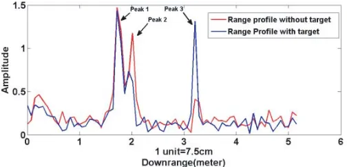
Before forming the 2D TWRI image of the target, it is essential to know the characteristics of the wall (i.e., dielectric constant), presence of the target, and its location. These things affect the quality of the image. Estimation of wall dielectric is done in a similar manner as proposed by Muqaible and Safaai-Jazi [16]. The dielectric value of the wall is found to be 6.4. For finding target location, the range profile at one of the scan points from the measured C-scan data using measurement setup is analyzed. The range profile can be represented as [15]

S(z) = 201

m=1

S(fk) exp(j2πfk(2z/c+Rdelay+2dwall(

√_ε

wall−1)/c)) ₍₁₄₎

whereRdelay is the delay due to antenna system,dwall the wall thickness, εwall the wall dielectric, and

fk the frequency. To estimate the delay due to the antenna system, a separate experiment has been

(7)

Figure 2. Range proﬁle plot.

of the C-scan data at which target reflections occurs. In the shown range profile plot, the first two peaks are due to reflections from the front and rear sides of the wall, and the third peak shows reflection from the target. Thus, the target downrange location has been calculated from the range profile.

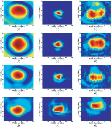
Once the wall parameter and target downrange position are estimated, the acquired C-scan data are further processed for the formation of 2D through-the-wall radar images using back projection, frequency wavenumber, and delay and sum beamforming. The two-dimensional image of the target (height vs cross-range) is plotted by considering a Y plane at a ﬁxed target range bin (z = ztarget)

which is selected by observing range profile. Thus, a virtual imaging plane of size 50×50 is created. Different imaging algorithms have been applied on acquired TWI data with various shapes of considered targets T1, T2, T3, and T4 to analyze the effect of the imaging. The 2D TWRI image of considered targets using each imaging algorithm is shown in Figures 3(a)–(l). In Figures 3(a)–(l),

X-axes represent cross-range, andY-axes represent the height of the target.

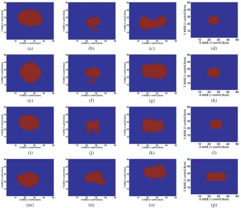
The shape of the target has been extracted after applying thresholding on the 2D TWRI using the statistical method [17]. The threshold value is calculated as

T h=mean+standard deviation (15) The thresholded 2D TWRI shape of considered targets using each imaging algorithm is shown in Figures 4(a)–(p) along with the reference shape of the target. The number of target pixels of reference target shape has been obtained based on a priori information of target size, location, and size of pixel [18– 20]. As per experimental results with various target samples, a considerable diﬀerence between the output images of algorithms from the focusing point of view is observed. From Figures 4(a)–(p), it is observed that though the considered imaging algorithm has accurately detected the position of the target, BP and F-K algorithms perform poorly in detecting approximate size and shape of the target. The shape and size of the target detected are compared with the reference target shape. The comparison between the number of target pixels detected using each imaging algorithm and the number of target pixels in reference target shape is shown in Table 3. From Table 3, it is observed that with the delay sum imaging technique, the numbers of target pixels detected are close to the number of target pixels of reference target shape as compared to frequency-wavenumber and backprojection imaging technique. This shows that delay and sum imaging algorithm proves to be a more eﬀective imaging tool than backprojection and frequency-wavenumber imaging algorithms for detecting approximate shape and size of the target.

(8)

(a) (b) (c)

(d) (e) (f)

(g) (h) (i)

(j) (k) (l)

Figure 3. (a) Raw 2D TWRI Image obtained using backprojectionimaging method on imaging plane along X and Y axis of target id T1. (b) Raw 2D TWRI Image obtained using delay and sum imaging method on imaging plane alongX andY axis of target id T1. (c) Raw 2D TWRI Image obtained using frequency wave number imaging method on imaging plane alongX andY axis of target id T1. (d) Raw 2D TWRI Image obtained using back projection imaging method on imaging plane alongXand Y axis of target id T2. (e) Raw 2D TWRI Image obtained using delay and sum imaging method on imaging plane along X and Y axis of target id T2. (f) Raw 2D TWRI Image obtained using frequency wave imaging number method on imaging plane along X and Y axis of target id T2. (g) Raw 2D TWRI Image obtained using backprojectionimaging method on imaging plane alongX andY axis of target id T3. (h) Raw 2D TWRI Image obtained using delay and sum imaging method on imaging plane along

(9)

(m) (n) (o) (p)

(i) (j) (k) (l)

(e) (f) (g) (h)

(a) (b) (c) (d)

Figure 4. (a) Raw 2D TWRI Image obtained using backprojection imaging method on imaging plane along X and Y axis of target id T1. (b) Raw 2D TWRI Image obtained using delay and sum imaging method on imaging plane alongX andY axis of target id T1. (c) Raw 2D TWRI Image obtained using frequency-wave number imaging method on imaging plane along X and Y axis of target id T1. (d) Reference target shape of target id T1. (e) Raw 2D TWRI Image obtained using backprojection imaging method on imaging plane alongX andY axis of target id T2. (f) Raw 2D TWRI Image obtained using delay and sum imaging method on imaging plane along X and Y axis of target id T2. (g) Raw 2D TWRI Image obtained using frequency-wavenumber imaging method on imaging plane along X andY

axis of target id T2. (h) Reference target shape of target id T2. (i) Raw 2D TWRI Image obtained using back projection imaging method on imaging plane along X and Y axis of target id T3. (j) Raw 2D TWRI Image obtained using delay and sum imaging method on imaging plane along Xand Y axis of target id T3. (k) Raw 2D TWRI Image obtained using frequency-wavenumber imaging method on imaging plane along X and Y axis of target id T3. (l) Reference target shape of target id T3. (m) Raw 2D TWRI Image obtained using backprojection imaging method on imaging plane along X and

(10)

Table 3. No. of target pixels detected in 2D TWRI of the considered target using diﬀerent imaging algorithm.

Targets

No. of targets pixels detected In

Backprojection image

No. of target pixels detected

In Delay Sum image

No. of target pixels detected In Frequency-Wavenumber

image

No. of target pixels in reference

target shape

T1 470 173 381 144

T2 470 210 466 196

T3 362 184 351 144

T4 362 272 342 240

Table 4. KS statistics and ﬁtting parameter for distributions of target image in 2D TWRI for target Id T1, T2, T3, and T4 for diﬀerent imaging algorithm.

Imaging

Algorithms Pdf Statistics Target T1 Target T2 Target T3 Target T4

Back-projection Beta

Statistics 0.02683 0.0176 0.01701 0.01944 P-value 0.87848 0.99815 0.9999 0.99881 Critical value 0.06264 0.06264 0.07137 0.07137

Fitting Parameters

α1 = 1.1474

α2 = 1.0165

a= 0.68875

b= 1.0

α1= 0.96525

α2= 0.81424

a= 0.68231

b= 1.0

α1= 0.94697

α2= 0.99075

a= 0.54975

b= 1.0

α1= 0.90775

α2= 1.0182

a= 0.51176

b= 1.0

Delay

and Sum Beta

Fitting Parameters

α1= 0.55899

α2 = 1.1222

a= 0.27584

b= 1.0125

α1= 0.62207

α2= 0.87022

a= 0.26461

b= 1.0

α1= 0.61138

α2= 1.0845

a= 0.3427

b= 1.0

α1= 0.75844

α2= 0.739

a= 0.39348

b= 1.0

Frequency-wavenumber Weibull

Fitting Parameters

α= 1.6266

β= 0.17504

γ= 0.60852

α= 3.7796

β= 0.38852

γ= 0.43273

α= 1.9381

β= 0.28158

γ= 0.41659

α= 1.287

β= 0.24285

γ= 0.42861

The pdf of the target image of the considered target for each imaging algorithm is shown in Table 4. From Table 4, it is observed that the probability distribution of the target images changes with imaging algorithm. For example, backprojection and beamforming have Beta distribution, whereas frequency-wavenumber has Weibull distribution. The probability density function of Weibull and Beta is given by [22]

f(x) = α

β

x−y β

α−1 exp

x−y β

α

(11)

whereα, β are shape parameters, andγ is the continuous location parameter.

f(x) = 1

B(α1, α2)

(x−a)α1−1(b−x)α2−1

(b−a)α1+α2−1 (17)

whereα1 and α2 are shape parameters, and aandb are continuous boundary parameters.

It is also observed that the pdf of the target image with delay sum imaging algorithm, back projection, and frequency-wavenumber imaging technique appears to consistently follow a single probability density function for diﬀerent considered targets. This shows that a single probability density based function captures the true properties of the backscattered signal. However, the shape parameter of weibull distribution changes with the small change in target geometry, and shape parameter of beta distribution remains almost constant with change in target geometry. This shows that a small change in target geometry provides a large change in the probability distribution of target image with a frequency-wavenumber algorithm, hence the possibility of the false alarms rate while performing detection of the target will be higher with frequency-wavenumber imaging algorithm and lower with backprojection and beamforming imaging technique.

Further, to analyze quality of 2D through-the-wall radar image of the target with these imaging algorithms, Peak to Signal Noise ratio (PSNR) is computed. PSNR is computed using Eqs. (14), (15) as

M SE = 1

M XN

N

i=1

M

j=1

(F(i, j)−I(i, j))2 (18)

P SN R(dB) = 10 log

1

M SE

(19)

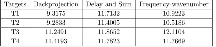
where I represents a 2D TWRI image without a target; F represents a raw 2D TWRI image with the target; M represents the number of pixels in row; and N represents the number of pixels in columns. The image quality of diﬀerent algorithms can be visibly observed from the obtained results. From Table 5, it is observed that peak to signal noise of formed images using delay and sum beamforming imaging technique is high and closely followed by backprojection and frequency-wavenumber imaging algorithm. A high PSNR shows that a good contrast is present between the pixels corresponding to the target and background pixels. Thus, the shape of the target can be easily detected.

Table 5. PSNR (dB) value of imaging algorithm for target id T1, T2, T3, T4.

Targets Backprojection Delay and Sum Frequency-wavenumber

T1 9.3175 11.7132 10.9223

T2 9.2833 11.4005 10.5186

T3 11.2491 11.8652 12.1104

T4 11.4193 11.7823 11.7669

(12)

observed that the probability distribution of the target images changes with the imaging algorithm. For example, backprojection and beamforming have Beta distribution, whereas frequency-wavenumber has Weibull distribution. Moreover, a small change in target geometry provides a large change in the shape parameters of Weibull distribution whereas shape parameters of Beta distribution do not change much with small change target geometry. It shows that the probability distribution of frequency-wavenumber image of target changes as target geometry changes, hence possibility of the false alarms rate will be higher with frequency-wavenumber imaging algorithm. Thus, delay and sum beamforming and backprojection algorithm are useful for detecting the location of a target with a low false alarm. However, backprojection and frequency-wavenumber imaging algorithms have poorly reconstructed approximate shape and size of the target compared to the delay and sum beamforming imaging algorithm. It has been observed that with delay and sum beamforming imaging technique, numbers of target pixels detected are close to the number of target pixels of reference target shape in comparison with frequency-wavenumber and backprojection imaging technique. Thus, delay and sum, and backprojection imaging algorithms can be used to detect the target with a low false alarm, but for detecting approximate shape and size of the target, delay and sum imaging algorithm proves to be a more eﬀective imaging tool than backprojection and frequency-wavenumber imaging algorithms.

3. DEVELOPMENT OF MODEL FOR SHAPE IDENTIFICATION OF TARGET

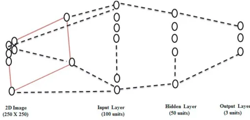
From the previous discussion, it has been observed that BP and F-K imaging techniques perform poorly in determining approximate shapes and sizes of the target as compared to delay and sum beamforming imaging techniques. Therefore, delay and sum beamforming imaging has been considered for the development of a target shape recognition model. The detected target images do not correspond to the actual shape and size of targets; therefore, there is a need for a methodology for the analysis of radar images, which can automatically perform recognition tasks and thereby help in decision making. Therefore, this 2D TWRI of the target using delay and sum beamforming imaging algorithm is further processed using an artificial neural network (ANN) to determine the actual shape of the target. The image formed has 50×50 pixels, which is a low-resolution image. The image resolution is increased by interpolation. Shape-preserving interpolation is used [17]. To identify the shape of the target, a feature that gives a description of target is required. The feature is extracted by applying 1D Wavelet Transform on the boundary of target. Shape identification of target can be achieved by comparing and matching the descriptors of the retrieved target image with descriptors of the synthetic image. One of the major problems which occurs in recognizing the shape of the targets is with its orientation. It is difficult to identify the particular shape of the target with a slight orientation effect. Thus, in order to make model orientation and scale-invariant, an orientation and scale-invariant feature is required. The feature is obtained by applying one-dimensional discrete wavelet transform (1D DWT) on the boundary of each shape. Using the 4-level Daubechies 1D DWT, the boundary of each shape described as (xi;yi)

is decomposed into approximated residual signals and detailed signals. This representation is presented as

x(m)

y(m)

= xa(m)

ya(m)

+

M

n=k

xdn(m)

ydn(m)

(20)

wherexa(m) andya(m) are the approximated residual signals, andxdn(m) andydn(m) are the detailed

signals corresponding to the mth point of the sequence. The approximated signals in terms of scaling functions φmk is gives as [23, 24]

xa(m) =

kakφM k(m)

ya(m) =

kckφM k(m)

(21)

where subscript M means the maximum level of decomposition, and k is the translation index. The detailed signals in terms of wavelet functions ψml are given as [21, 22]

xdn(m) =

nrpnψpn(m)

ydn(m) =

ndpnψpn(m)

(13)

where subscriptsp= 1,2, . . . , M mean the succeeding levels of decomposition. The wavelet descriptors are created here by coeﬃcients an, cn, representing the approximated signal and by the set of rpndpn

(p= 1,2, . . . , M), representing the detailed signals of M applied levels of decomposition.

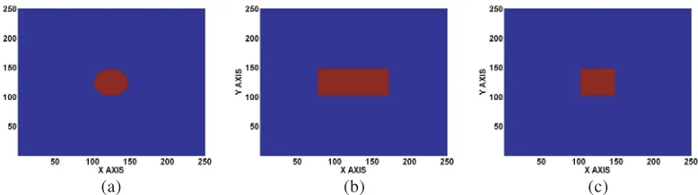
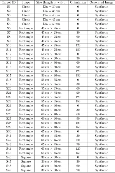
The complete WT features are arranged into one-dimensional vector. These features are further normalised, making them independent of the scale and orientation [24]. As a result of such normalization, we get wavelet descriptors invariant to the scale and rotation. Further, to make the feature vector compact, the first 100 coefficients are selected from the rest of the descriptor without losing relevant information of the target. This feature provides the identity to shape of the target. With the use of these descriptors, the target can be discriminated. After feature vectors are obtained, these feature vectors will be fed to ANN for training. Although many classifiers are available in the literature, neural network is very promising over other classifiers. Further, to increase the detection accuracy of the ANN model, a lot of training data are required. Therefore to increase data, synthetic data of three common shapes of various sizes and orientations of target are generated using Boolean values as given in Appendix A [18, 19]. The synthetic target shape has been obtained based on a priori information of target size, location, and size of pixel [20]. For example, synthetic data of rectangular shape of sizes (50×30), (45×25) cm, (55×35) cm, (60×40) cm, and (65×45) at orientations 0, 30, 60, 90, 120, 150, and 180 degrees have been generated. Similarly, synthetic data of square shape of sizes (30×30), (35×35) cm (40×40) cm, (45×45) cm, and (50×50) cm at orientations 0, 30, 60, 90, 120, 150, and 180 degrees have been generated, and synthetic data of circle shape of sizes (30×30), (35×35) cm (40×40) cm, (45×45) cm, and (50×50) cm at orientation 0 have been generated. The number of target pixels in the synthetic image is obtained based on a priori information of target size, location, and size of pixel [16]. Figures 5(a), (b) & (c) show synthetic image of circular, square, and rectangular shapes of sizes 30 cm× 30 cm, 30 cm ×30 cm, and 50 cm ×30 cm. In Figure 5, X-axis represents the height, and Y-axis represents the horizontal cross-range. OnX and Y axes, pixel points are shown having 1 unit = 0.5 cm.

(a) (b) (c)

Figure 5. (a) Synthetic image of the circular shape of size 30 cm. (b) Synthetic image of the rectangle shape of size 50 cm ×30 cm. (c) Synthetic image of the square shape of size 30 cm ×30 cm.

(14)

Figure 6. Neural network conﬁguration for shape identiﬁcation.

neural network which is deﬁned as

mse= 1

N

i=1

e2i =

1

N

i=1

(ri−ai)2 (23)

where ‘a’ is the network outputs, and ‘r’ is the target outputs. In MSE criteria the neural network ﬁrst produces its own output vector ‘a’ according to fed input vector and then compares the output vector with the desired target vector ‘t’. If an error occurs, then the weights are adjusted using the scaled conjugate gradient method to reduce the diﬀerence until MSE reaches below 0.01 for optimum performance. The performance of the neural network is better for the lower value of mean square error.

Table 6. List of real independent target samples used for testing of neural network.

Target ID Shape Size (Length×Width) Orientation Material RT1 Square 30 cm×30 cm 0 Wood

RT2 Square 35 cm×35 cm 135 Wood RT3 Rectangle 50 cm×30 cm 0 Wood RT4 Rectangle 50 cm×30 cm 45 Wood

RT5 Rectangle 55 cm×35 cm 135 Wood RT6 Square 30 cm×30 cm 45 Metal RT7 Square 35 cm×35 cm 0 Metal

RT8 Rectangle 50 cm×30 cm 45 Metal RT9 Rectangle 55 cm×35 cm 135 Metal RT10 Circle Dia = 35 cm 0 Metal

(15)

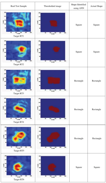
Table 7. Results of developed ANN model with independent test data sample.

Real Test Sample Thresholded image Actual Shape

Square

Rectangle

Rectangle Shape Identified

using ANN

Square

Rectangle

Rectangle Target RT1

Target RT2

Target RT3

Target RT4

Rectangle

Square Rectangle

Square Target RT5

(16)

Square

Rectangle

Rectangle Square

Rectangle

Rectangle Target RT7

Target RT8

Target RT9

Target RT10

Circle Circle

diﬀerent irregular target shapes. As a future work plan, more sophisticated and practical target shapes will be considered for shape recognition.

4. CONCLUSION

(17)

APPENDIX A.

Table A1. List of samples used for training of neural network.

Target ID Shape Size (length ×width) Orientation Generated Image

S1 Circle Dia = 30 cm 0 Synthetic

S6 Rectangle 45 cm×25 cm 0 Synthetic

S46 Square 30 cm×30 cm 0 Synthetic

(18)

S50 Square 30 cm ×30 cm 120 Synthetic

REFERENCES

1. Baranoski, E. J., “Through-wall imaging: Historical perspective and future directions,”Journal of the Franklin Institute, Vol. 345, 556–569, 2008.

2. Smith, G. E. and B. G. Mobasseri, “Robust through-the-wall radar image classiﬁcation using a target-model alignment procedure,” IEEE Transactions on Image Processing, Vol. 21, 754–767, 2011.

3. Hantscher, S., B. Praher, A. Reisenzahn, and C. G. Diskus, “Comparison of UWB target identiﬁcation algorithms for through-wall imaging applications,”IEEE European Radar Conference, 104–107, 2006.

4. Kidera, S., T. Sakamoto, and T. Sato, “High-resolution 3-D imaging algorithm with an envelope of modiﬁed spheres for UWB through-the-wall radars,” IEEE Transactions on Antennas and Propagation, Vol. 57, 3520–3529, 2009.

5. Dogaru, T. and C. Le, Through-the-wall Small Weapon Detection Based on Polarimetric Radar Techniques, Army Research Lab Adelphi MD Sensors and Electronic Devices Directorate, No. ARL-TR-5041, 2009.

(19)

7. Wu, S., Y. Xu, J. Chen, S. Meng, G. Fang, and H. Yin, “Through-wall shape estimation based on UWB-SP radar,”IEEE Geoscience and Remote Sensing Letters, Vol. 10, 1234–1238, 2013.

8. Dehmollaian, M., “Through-wall shape reconstruction and wall parameters estimation using diﬀerential evolution,”IEEE Geoscience and Remote Sensing Letters, Vol. 8, 201–205, 2010. 9. Ahmad, F., M. G. Amin, and S. A. Kassam, “Synthetic aperture beamformer for imaging through

a dielectric wall,”IEEE Transactions on Aerospace and Electronic Systems, Vol. 41, 271–283, 2005. 10. Hunt, A. R., “Use of a frequency-hopping radar for imaging and motion detection through walls,”

IEEE Transactions on Geoscience and Remote Sensing, Vol. 47, 1402–1408, 2009.

11. Ahmad, F., Y. Zhang, and M. G. Amin, “Three-dimensional wideband beamforming for imaging through a single wall,” IEEE Geoscience and Remote Sensing Letters, Vol. 5, 176–179, 2008. 12. Hantscher, S., B. Praher, A. Reisenzahn, and C. G. Diskus, “Analysis of imaging radar algorithms

for the identiﬁcation of targets by their surface shape,”Int. Conf. on UWB, 2006.

13. Yigit, E., S. Demirci, C. Ozdemir, and A. Kavak, “A synthetic aperture radar-based focusing algorithm for B-scan ground penetrating radar imagery,” Microwave and Optical Technology Letters, Vol. 49, 2534–2540, 2007.

14. Ozdemir, C., S. Demirci, and E. Yigit, “Practical algorithms to focus B-scan GPR images: Theory and application to real data,”Progress In Electromagnetics Research B, Vol. 6, 109–122, 2008. 15. Verma, P. K., A. N. Gaikwad, D. Singh, and M. J. Nigam, “Analysis of clutter reduction techniques

for through wall imaging in UWB range,”Progress In Electromagnetics Research B, Vol. 17, 29–48, 2009.

16. Muqaibel, A. H. and A. Safaai-Jazi, “A new formulation for characterization of materials based on measured insertion transfer function,” IEEE Transactions on Microwave Theory and Techniques, Vol. 51, 1946–1951, 2003.

17. Chandra, R., A. N. Gaikwad, D. Singh, and M. J. Nigam, “An approach to remove the clutter and detect the target for ultra-wideband through-wall imaging,”Journal of Geophysics and Engineering, Vol. 5, 412–419, 2008.

18. Singh, D., N. K. Choudhary, K. C. Tiwari, and R. Prasad, “Shape recognition of shallow buried metallic objects at X-band using ANN and image analysis techniques,”Progress In Electromagnetics Research B, Vol. 13, 257–273, 2009.

19. Ibrahim, K. M., K. F. A. Hussein, and A.-E.-H. A.-E.-A. Ammar, “Land-buried object detection and target-shape recognition in lossy and dispersive soil,” Progress In Electromagnetics Research B, Vol. 57, 279–298, 2014.

20. Kumar, B., R. Upadhyay, and D. Singh, “Development of an adaptive approach for identiﬁcation of targets (match box, pocket diary and cigarette box) under the cloth with MMW imaging system,” Progress In Electromagnetics Research B, Vol. 77, 37–55, 2017.

21. “Easyfit by mathwave technologies,” [Online]. Available:http://www.mathwave.com/easyfit-distribution-fitting.html.

22. Forbes, C., E. Merran, H. Nicholus, and P. Brian,Statistical Distributions, John Wiley and Sons, New Jersey, 2011.

23. Gonzalez, S. and W. Richards, Digital Image Processing, Dorling Kindersley, New Delhi, 2009. 24. Osowski, S., “Fourier and wavelet descriptors for shape recognition using neural networks — A

comparative study,”Pattern Recognition, Vol. 35, 1949–1957, 2002.